Article

Joint Optimization of Intersection Control and Trajectory Planning Accounting for Pedestrians in a Connected and Automated Vehicle Environment

1
Laboratoire Ville Mobilité Transport, École des Ponts ParisTech, 77455 Marne-la-Vallée CEDEX 2, France
2
Division of Engineering, New York University Abu Dhabi, Abu Dhabi P.O. Box 129188, United Arab Emirates
3
Department of Aeronautics and Astronautics, Stanford University, Stanford, CA 94305, USA
*
Author to whom correspondence should be addressed.
Sustainability 2021, 13(3), 1135; https://doi.org/10.3390/su13031135
Submission received: 31 December 2020 / Revised: 17 January 2021 / Accepted: 19 January 2021 / Published: 22 January 2021

Abstract

:
Connected and automated vehicle (CAV) technology makes it possible to track and control the movement of vehicles, thus providing enormous potential to improve intersection operations. In this paper, we study the traffic signal control problem at an isolated intersection in a CAV environment, considering mixed traffic including various types of vehicles and pedestrians. Both the vehicle delay and the pedestrian delay are incorporated into the model formulation. This introduces some additional complexity, as any benefits to pedestrians will come at the expense of higher delays for the vehicles. Thus, some valid questions we answer in this paper are as follows: Under which circumstances could we provide priority to pedestrians without over penalizing the vehicles at the intersection? How important are the connectivity and autonomy associated with CAV technology in this context? What type of signal control algorithm could be used to minimize person delay accounting for both vehicles and pedestrians? How could it be solved efficiently? To address these questions, we present a model that optimizes signal control (i.e., vehicle departure sequence), automated vehicle trajectories, and the treatment of pedestrian crossing. In each decision step, the weighted sum of the vehicle delay and the pedestrian delay (e.g., the total person delay) is minimized by the joint optimization on the basis of the predicted departure sequences of vehicles and pedestrians. Moreover, a near-optimal solution of the integrated problem is obtained with an ant colony system algorithm, which is computationally very efficient. Simulations are conducted for different demand scenarios and different CAV penetration rates. The performance of the proposed algorithm in terms of the average person delay is investigated. The simulation results show that the proposed algorithm has potential to reduce the delay compared to an actuated signal control method. Moreover, in comparison to a CAV-based signal control that does not account for the pedestrian delay, the joint optimization proposed here can achieve improvement in the low- and moderate-vehicle-demand scenarios.

1. Introduction

Traffic signal control is crucial for intersection management. As reported in [1], annual delays at traffic signals on major roadways are estimated to be around 295 million vehicle-hours in the United States. Traditionally, either historical data are used in fixed-time control schemes or real-time information from loop detectors is used for actuated or adaptive control. The recent development of connected and automated vehicle (CAV) technology (i.e., data exchange by the means of intervehicle and vehicle–infrastructure communications) makes it possible to track and control the movement of vehicles. Using CAV technology, intersection control efficiency can be improved, not only with the real-time data acquisition but also with the cooperation of intersection control and vehicle trajectory planning. Studies show that traffic control schemes for signalized or unsignalized intersections under a CAV environment are far superior to the conventional traffic signal timings [2,3,4,5].
CAV data can be useful for traffic signal optimization. The data generally include the real-time positions and motion of vehicles. By processing the data, traffic state-related variables such as vehicle density and queue length can be estimated [6] and then used for adaptive signal control at intersections [7,8,9,10]. Such control can also take into account vehicle platooning [3,11]. In recent years, abundant literature has focused on the intersection control under a CAV environment. The methods can be mainly classified into two categories. In the first category, cooperative resource reservation systems are proposed to schedule resources at unsignalized intersections, regarding time slots and space tiles [2,12,13,14]. CAV trajectory planning is applied to avoid collisions of vehicles at the intersections. The second category focuses on the optimization of vehicle departure sequences [4,15,16,17]. In some studies, the departure sequence is also represented by the changes in signal phases at signalized intersections, considering mixed traffic streams with conventional vehicles and various penetration levels of CAVs [3]. Some approaches use the joint optimization of signal timings (or vehicle departure sequence) and CAV trajectory planning to improve the control efficiency [18,19]. Although the joint optimization leads to a much better intersection performance, it normally demands high computational costs. The problem complexities come from the large size of signal phase states (or all possible departure sequences) and the uncertainty associated with the vehicle motion profiles, especially when not all vehicles are automated. To solve these computational issues, multiple alternatives have been used to find the jointly optimal or near-optimal solution, including heuristic algorithms [19], dynamic programming [20], and mathematical programming [21,22]. Other strategies to improve computational efficiency include using simple trajectory segments to reduce control variables [23], and formulating short-term driving plans [24]. However, most of the literature on this joint optimization only considers the full penetration of CAVs, with only a few exceptions [19,21]. It is worth mentioning that the joint optimization can lead to significant improvements in traffic efficiency for low and moderate traffic demands, but it becomes less efficient in high-vehicle-demand scenarios due to increased uncertainty [18,19].
Generally, an urban intersection manages motorized (i.e., vehicles or transit) and nonmotorized traffic participants (i.e., pedestrians or cyclists). Although pedestrians and other vulnerable road users have received significant attention for intersection management, all the CAV studies mentioned above only focused on the motorized modes.
Intersection operations accounting for the interaction between pedestrians and vehicles have already been modeled, although mostly without CAVs [25,26,27,28]. A tradeoff exists between pedestrians and vehicles. Evidence shows that reduced pedestrian delay and improved safety normally come at the expense of traffic efficiency, especially in high-vehicle-demand scenarios [27,28,29]. This makes sense because giving any priority to pedestrians with high vehicle demands will impose a large penalty to vehicles (those might be delayed for multiple signal cycles) while providing very little benefit to an average pedestrian (who will never have to wait more than one cycle—as there is no strict capacity restriction for them to cross the street once they get the green light). That being said, even when providing priority to pedestrians, it is still possible to optimize intersection control systems by adjusting traffic signal timings or operation modes. Kothuri et al. [30] argued that the traffic-volume-to-road-capacity ratios coupled with pedestrian actuation frequency for signal phases could be used to determine the signal controller’s mode of operation to produce the lowest system delay. To manage intersections comprehensively, the optimization problems of traffic signal timings considering pedestrian delay have already been studied in the context of human-driven (i.e., conventional) vehicles [31,32,33]. CAVs have mostly been included in pedestrians’ intention to pass the crosswalk [34,35]. However, to the best of our knowledge, there is no pedestrian delay model considered for intersection control under a CAV environment. The control efficiency of automated vehicles (AVs) in the presence of pedestrians crossing is unclear. In summary, the joint optimization of traffic signal timings, pedestrian crossing, and vehicle trajectory planning has not been studied yet. We also found that the existing control strategies of CAVs only focus on pedestrian safety aspects, while they fail to pay enough attention to the efficiency aspect, i.e., pedestrian delay.
To close this research gap, our study aims to combine traffic signal control for both vehicles and pedestrians at intersections with CAV technology. We build on the work by Yang et al. [19] and incorporate pedestrian crossing, monitoring, and evaluation. The contributions of this paper are threefold. First, this work proposes a pedestrian delay model that is combined with a vehicular delay model in a joint framework, which optimizes the traffic signal control problem. Second, we shed light on the benefits of CAVs with increases of the penetration rates in relation to pedestrian crossing at the intersection. Third, we develop an ant colony system (ACS) algorithm to find a near-optimal solution of the integrated problem with high computational efficiency. In this study, we focus on the general insights regarding the actual value of considering crossing pedestrians. To this end, we look at a relatively simple case to understand the value of accounting for pedestrian delay in different scenarios.
The remainder of this paper is organized as follows: Section 2 presents the integrated optimization problem of traffic signal control with pedestrians and AV trajectory planning. Section 3 introduces the ACS solution for the integrated problem. Section 4 introduces the simulation environment. Section 5 analyzes the feasibility of the ACS algorithm and the reliability of the vehicle and pedestrian delay models. Section 6 evaluates the performance of the control algorithm and compares it with an actuated signal control algorithm. Section 7 concludes the paper by providing some final remarks.

2. Integrated Optimization Problem

Using the information obtained from CAVs, the signal control algorithm is developed for an isolated intersection with multiple straight traffic streams and pedestrian movements. The studied intersection has four legs, and each leg has a crosswalk with two sidewalks to hold pedestrians, as shown in Figure 1. There are two signal phases for the two groups of vehicle movements at opposite approaches. They also include two groups of pedestrian movements associated with the different vehicle movements.
Three categories of vehicles are considered: (1) conventional vehicles, (2) automated vehicles, and (3) connected vehicles (CVs). Conventional vehicles cannot send vehicle information to the central controller. AVs are the vehicles without a driver, whose trajectories can be controlled by the central controller and the automated driving system. Although all AVs provide information (i.e., are connected), we call CVs only those vehicles that send information to the central controller, but whose trajectories cannot be controlled/modified. It is assumed that both CVs and AVs are equipped with vehicle-to-infrastructure (V2I) communication systems to send and receive information in relation to the intersection via dedicated short-range communications (DSRC). Such exchange of information happens within a limited area, herein called the zone of interest. It is unrealistic to have the length of the zone of interest longer than a city block, as this would require a priori information on route choice. It is also required for the zone of interest to be within the DSRC transmission range (normally within 100–1000 m) due to physical constraints. Thus, we assume that the zone of interest is defined by a 100 m radius around the intersection (this choice is rather conservative; the performance is expected to improve by increasing this length, as there is more information provided by CAVs [23]), and that there is no delay for CVs and AVs to send and receive information. Similarly to [19], in our study, the information level rinfo is defined as the ratio of all equipped vehicles (i.e., CAVs = CVs + AVs) to the total number of vehicles, and the automated level rauto is defined as the ratio of AVs to all equipped vehicles. These two metrics reflect the penetration rate of CAVs and can be used to represent different implementation stages of new vehicle technologies.
At a signalized pedestrian crosswalk, a pedestrian signal cycle usually consists of three signal display intervals: “walk (W)” interval, “flashing do not walk (FDW)” interval, and the steady “do not walk (DW)” interval. The W interval (i.e., pedestrian green signal) indicates that it is safe for pedestrians to cross. The FDW interval implies that no additional pedestrians should start to cross. Generally, FDW is estimated by a minimum pedestrian crossing time, which is equal to the crossing length divided by the expected walking speed (normally 1.2 m/s). FDW is followed by a yellow interval in some cases. The FDW in our study is followed by an all-red interval, and the yellow interval is included in this all-red clearance time. Hence, the pedestrian clearance (PC) interval is the sum of the FDW and the all-red time of pedestrian signals (see Figure 3, Section 2.2.2). The DW interval (i.e., pedestrian red signal) is the time period during which pedestrians do not have the right of way as assigned by the signal.

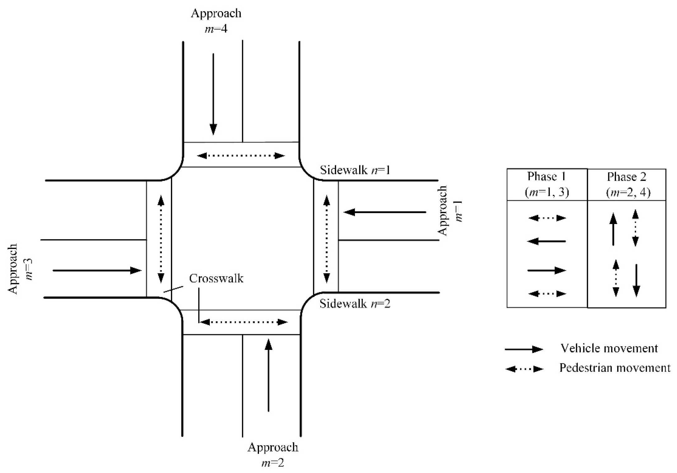
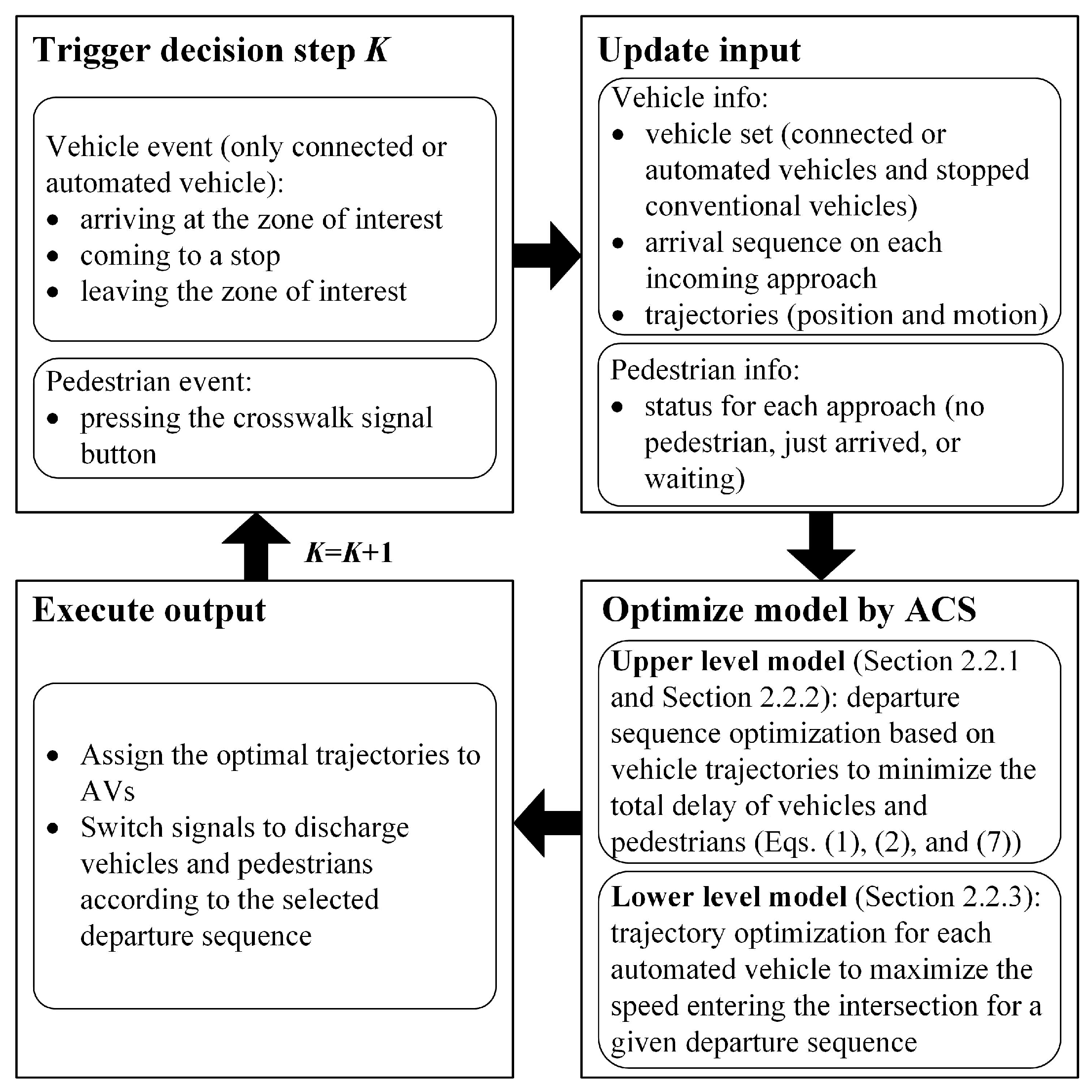
2.1. Model Framework

The model framework for cooperative traffic and pedestrian signal control is shown in Figure 2. There are four stages within each decision step. The decision-making within the controller is an event-based control process.
In the first stage, we consider four triggering events: (1) a connected or automated vehicle entering the zone of interest, (2) a connected or automated vehicle coming to a stop, (3) a connected or automated vehicle leaving the zone of interest, and (4) a pedestrian pressing the crosswalk signal button. The first three events are vehicle events and the last one is a pedestrian event. We assume that, as in reality, the crosswalk signal button is pressed at most once within each cycle, and this is done by the first pedestrian arriving during FDW or DW for a given approach on either sidewalk.
Each of the four events described above triggers a decision process and updates the model inputs, which include vehicle and pedestrian information. The vehicle information includes (1) the vehicle set that consists of all CAVs in the zone of interest and the stopped conventional vehicles ahead of some stopped CAVs (they are estimated through the locations of CAVs), (2) the arrival sequence, and (3) the observed or estimated trajectory of each vehicle. Notice that the arrival sequence of conventional vehicles can be estimated using the location information of connected and automated vehicles. Once a connected or automated vehicle comes to a stop, the number of conventional vehicles stopping in front of it (i.e., the arrival sequence of conventional vehicles) can be estimated by kinematic wave theory (given previous signal settings and assuming a fundamental diagram). The estimation accuracy increases with the penetration rate of CAVs. Details on the estimation process can be found in [6]. The pedestrian information consists of the status of waiting pedestrians for each of the approaches (on either sidewalk): a pedestrian has just arrived triggering the decision process, at least one pedestrian is already waiting (i.e., they have arrived in a previous event), or there is no pedestrian at all. The event is only triggered when the first pedestrian arrives and presses the button at a given approach. The pedestrian event remains active until the pedestrian gets a W signal to actually cross the intersection.
In the third stage, we propose a bilevel optimization model that integrates the optimization of departure sequences (accounting for vehicle and pedestrian departures) and the trajectory design for AVs. In the upper level, the departure sequence is (nearly) optimized (yielding the corresponding signal changes) to minimize the total delay of vehicles in the zone of interest and pedestrians at the intersection. In the lower level, the trajectory of each AV is optimized for a given departure sequence to maximize the speed entering the intersection. Hence, the two levels interact with each other. In this study, the bilevel model is solved by an ACS algorithm to gain computational efficiency.
In the final stage, AVs are given the designed trajectories from the lower-level model, and the central controller changes signals to discharge vehicles and pedestrians, according to the selected departure sequence from the upper-level model. New decision steps in the algorithm are triggered every time an event occurs, and the whole optimization is revised. The traffic signal does not operate with a constant cycle length, but with an actuated control logic, according to the detection of vehicles and pedestrians, as well as the optimized departure sequence.

2.2. Model Formulation

In this subsection, we introduce the joint optimization problem, where the objective function aims to minimize the total combined vehicle and pedestrian delay, defined in Equation (1). For the readers’ convenience, the most important notation used here is listed in Table 1.
In the joint optimization problem, we look for the departure sequence J that minimizes the total combined vehicle and pedestrian delay in Equation (1).
min J ( ( 1 ω ) · Delay J veh + ω · Delay J ped ) ,
where ω ( 0 ω < 1 ) is the weight used between the vehicle delay Delay J veh and the pedestrian delay Delay J ped for a given departure sequence J. ω can be a function of average vehicle occupancy or any specific prioritization policy (e.g., for the case where both delays are treated the same and the average vehicle occupancy is assumed to be 1, then ω = 0.5). We next provide the formulations for the vehicle delay (Section 2.2.1), the pedestrian delay (Section 2.2.2), and the AV trajectory design (Section 2.2.3).

2.2.1. Vehicle Delay

For each vehicle c within a vehicle set N ( c N ), we consider three properties: (1) the position index i in the arrival sequence I ( i I ), (2) the position index j in the departure sequence J ( j J ), and (3) the incoming approach m ( m M ). The arrival sequence i and the approach m are based on the initial detection or assumption of a vehicle’s location. The optimal departure sequence is determined on the basis of the departure sequence algorithm (introduced in Section 3).
For each departure sequence J, the total vehicle delay is calculated as the sum of all individual vehicle delays (see Equation (2)). For each vehicle c, we estimate the vehicle delay using the difference between the predicted departure D c , J under sequence J and the virtual departure time V c . D c , J is calculated on the basis of Newell’s car-following model and the trajectory design proposed in our study (if c is an automated vehicle). V c is an ideal departure time at which the vehicle would depart the intersection in the absence of any queue/delay, and it is calculated by the distance from the current location to the departure line of the intersection divided by the free-flow speed at a given approach. Note that, in each decision step, the predicted departure time D c , J can be changed by control policies as long as the vehicle has not departed from the intersection. Thus, it is not really an actual departure time but close to it. According to Equation (2), the estimation of total vehicle delay can be changed correspondingly as the vehicle trajectories are updated by control policies. The validation of estimated results with actual vehicle delay can be seen in Section 5.
Delay J veh = c N ( D c , J V c ) .
For a given departure sequence J and the corresponding optimal trajectories of AVs, the predicted departure time D c , J for vehicle c = { i , j , m } , c N is calculated as the maximum of the virtual departure time and the next possible departure time (i.e., the right expression in the parentheses in Equation (3)). That is,
D c , J = { max { V c ; D c , J + 1 s m + P c , J } , If c and c are in the same signal phase max { V c ; C c , J + P c , J } , Otherwise ,
where c is the vehicle prior to vehicle c in this departure sequence, s m is the vehicle saturation flow rate for the approach of interest, P c , J is a delay penalty to account for the effects of vehicle platooning, and C c , J is the start time of the signal phase that allows vehicle c to c depart from the intersection. Notice that the first statement of Equation (3) only considers that c and c are in opposite flows that have the same signal phase. Otherwise, D c , J + 1 / s m should be replaced by C c , J , which is determined by the maximum of the departure time of vehicle c on the conflict approach of vehicle c and the time that allows pedestrians to cross through the approach that vehicle c is associated with. Moreover, the duration of a pedestrian clearance interval is added in order to guarantee the safety of pedestrians crossing. We define C c , J = max { D c , J , C c , J + Δ t W min } + Δ t PC , where Δ t W min is the minimum pedestrian green time and Δ t PC is the duration of pedestrian clearance interval. The delay penalty P c , J is derived using basic kinematic laws, as shown in Equation (4).
P c , J = max { l u f ; u c , J init + ( u c , J init ) 2 + 2 a l a } ,
where l is the length of the intersection, u f is the free-flow speed, a is the acceleration, and u c , J init is the initial speed of vehicle c when entering the intersection. The initial speed u c , J init is the result of the trajectory optimization for AVs (introduced in Section 2.2.3). Notice that the farther behind a vehicle is within the platoon, the higher its initial speed when departing from the intersection. Thus, its penalty cost is less, according to Equation (4). As a result, even though vehicle platoons are not explicitly considered in Equation (4), this penalty function does encourage discharging in platoons [3,19].

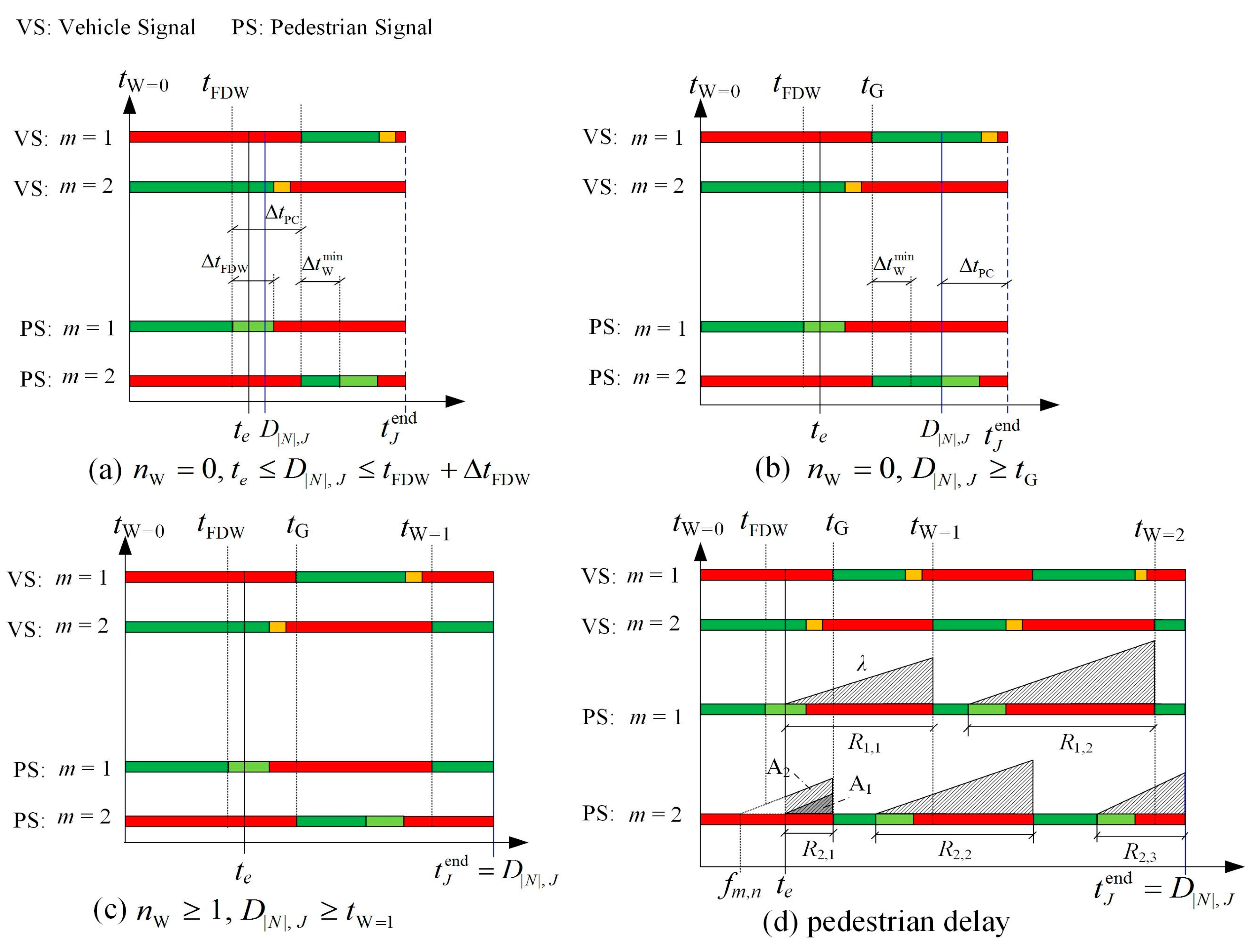
2.2.2. Pedestrian Delay

The pedestrian delay model presented here is based on three main assumptions: (1) a pedestrian event occurs when the first pedestrian gets to press the button on condition that the crosswalk signal is FDW or DW for their approach; (2) the pedestrian delay only includes the waiting time for crossing and does not include the delay from the pedestrians’ discharge and walking time at crosswalks or across the intersection (pedestrians immediately enter the crosswalk but only when a W signal provides the right of way); (3) the predicted pedestrian arrivals follow a uniform process. Assumption (1) indicates that, as in reality, the pedestrian signal button is pressed to be valid at most once within the pedestrian signal cycle of each crosswalk (the button is pressed at any of the two sidewalks for any given crosswalk). Assumption (2) simplifies the delay model without accounting for pedestrian start-up delay and pedestrian saturation flow rate. The observed pedestrian queue discharge capacity (e.g., 4.2 pedestrians/s in a crosswalk of 3 m width) is much higher than the vehicle queue discharge capacity (e.g., 0.5 vehicles/s in a similar width) [36]. That is why the pedestrian delay model can ignore the start-up impact while the vehicle delay model cannot. Assumption (3) simplifies the calculation but does not imply that pedestrians arrive in a uniform pattern. As a matter of fact, for the simulation, we later assume that pedestrians arrive following a Poisson process. Notice that pedestrians who arrive randomly do not provide any type of arrival information to the controller, except the first arriving pedestrian who presses the button. In the pedestrian delay model, we adopt Assumption (3) to estimate the delay of pedestrians who arrive during the planning horizon. The pedestrian delay model used in this section builds on a simple model from the Highway Capacity Manual (HCM) [37], which calculates the pedestrian delay on the basis of a triangular area rule, assuming that the signal cycle is fixed. As our algorithm aims to optimize the vehicle departure sequence, we extend the HCM model to account for variable signal cycles. In other words, we improve the HCM model to estimate the pedestrian delay according to different vehicle departure sequences, which change the pedestrian delay calculation period. The estimation of the calculation period is mainly determined by the predicted departure time of the last vehicle in the departure sequence J, as well as the vehicle and pedestrian signal status. These factors increase the complexity of the pedestrian delay estimation.
Once a vehicle or pedestrian event happens, the optimization process starts. To estimate pedestrian delay, we first need to determine the estimation horizon, which goes from the start time of a vehicle or pedestrian event t e to the ending time of the pedestrian delay calculation t J end . The predicted discharge time of all vehicles in a given departure sequence J is the interval starting with the vehicle or pedestrian event occurring at time t e and ending with the last vehicle departure time D | N | , J . If there are no waiting pedestrians, we only forecast the pedestrian delay during the total discharge time of the vehicles in J (i.e., [ t e , D | N | , J ]). Otherwise, a longer period [ t e , t J end ] might be considered, so that any pedestrian already waiting can also discharge (assuming a minimum pedestrian crossing time Δ t W min for safety purposes). t e is an input, and D | N | , J is a function of the vehicle departure sequence J (see Equation (3)). t J end is computed below for events triggered by a pedestrian.
In the four-legged intersection as shown in Figure 1, traffic on approach m = 1 and its opposite approach m = 3 is a set of compatible movements, and the same applies for traffic on approach m = 2 and its opposite approach m = 4. As opposite approaches can always get the same signal plan, here, we only illustrate the signal plan of two conflicting approaches, i.e., m = 1 and m = 2 related to phase 1 and phase 2, respectively. Focusing on pedestrian signals on relevant approaches (for ease of use, the pedestrian signal of a crosswalk is deemed as the one related to the approach that is in the same leg of the intersection), as shown in Figure 3, the W signal appears alternatively between approach m = 1 and approach m = 2 according to the vehicle departure sequence J. Because of symmetry, only one approach of the two conflicting approaches is discussed here (i.e., the reference approach). We consider the reference approach that one where a pedestrian arrives and the pedestrian event is triggered. For the derivations below, we assume that approach m = 1 is the reference approach. The triggering pedestrian event can then only happen in the first ongoing FDW interval or DW interval of approach m = 1.
t J end is then defined as:
t J end = { t FDW + Δ t W min + 2 Δ t PC , if n W = 0 , N = t e D | N | , J t FDW + Δ t FDW max { D | N | , J , t G + Δ t W min } + Δ t PC , if n W = 0 , t G , D | N | , J t G D | N | , J , if n W 1 , t W = 1 , D | N | , J t W = 1 ,
where n W is the number of signal changes to W for the reference approach during time interval [ t e , D | N | , J ], t W = k is the time associated with the kth W signal start time for the reference approach, t FDW and t G are the start time of FDW and the green signal for vehicles on the reference approach when n W = 0, respectively, Δ t W min is the minimum pedestrian crossing time, and Δ t PC is the length of the pedestrian clearance interval. If the triggering pedestrian event happens in approach m = 2, Equation (5) still holds. The explanation of Equation (5) is given below.
In Figure 3a,b, where n W = 0 , t J end represents an extension of D | N | , J , except the case of N = . In the prediction, the pedestrian signal for the reference approach should change to W in the next cycle, in order to guarantee the departure of any pedestrian that has triggered the current event (this also explains the case of N = ). Such a signal change should happen after the other approach (m = 2) safely discharges any pedestrian that might (have) arrive(d). The W for m = 2 (i.e., t G ) will start at least after t FDW + Δ t PC , and the minimum pedestrian crossing time is Δ t W min . If t G is not known yet (see Figure 3a), t J end is calculated with the first statement of Equation (5) where we already know t FDW ; otherwise (see Figure 3b), it is calculated with the second statement of Equation (5). In Figure 3c, we have n W = 1 and then t J end = D | N | , J (the third statement of Equation (5)). This is because the pedestrians on the reference approach will have a chance to get a W signal within the computed vehicle departure sequence J, and they can discharge immediately (see Assumption (2)).
Notice that there might already be some pedestrians waiting by the time the new event happens at t e . We call this “active repetition”, which means that the current event is triggered by a vehicle or a pedestrian while previous pedestrian events are still active. There are two possible cases of active repetition. One case happens when the current event is triggered by a vehicle while pedestrian events are still active (i.e., the pedestrians have not discharged yet). In that case, we do not use Equation (5) and go directly to Equation (6) below, using for this approach t J end equal to the maximum value between D | N | , J and the t J end computed from the last pedestrian event. The other case happens when the current event is triggered by a pedestrian, but their approach is different from the approach(es) where previous pedestrian events are still active. In both cases, we need to make sure that we use the largest t J end obtained across all of those pedestrian events that are still active, as shown in Equation (6).
t J end = max m M { t J , 1 end , t J , 2 end , , t J , m end } ,
where m ( 1 m 4 ) is the approach for which a pedestrian event is active by the time t e .
According to the triangular area rule, the pedestrian delay is then calculated by λ R 2 / 2 , where λ is the pedestrian arrival rate and R is the effective pedestrian red time. In our study, we consider the pedestrian delay during the term [ t e , t J end ] for the vehicle departure sequence J, which might include multiple R intervals (e.g., Figure 3d). In particular, for the case of active repetition, the delay of the first R on an approach, where the pedestrian event is already active, is represented by a trapezoidal area (i.e., A2 in Figure 3d) rather than the triangular area (i.e., A1 in Figure 3d), which refers to the case of no active repetition. The total pedestrian delay at the intersection is the sum of the expected delays on both sidewalks (n = 1, 2) of each leg, and it is estimated with Equation (7).
Delay J ped = m = 1 , 2 , 3 , 4 n = 1 , 2 ( r = 1 n r λ m , n R m , r 2 2 + λ m , n ( t e f m , n ) R m , 1 ) ,
where R m , r is the r-th pedestrian waiting interval in approach m, and n r is the number of R m , r within [ t e , t J end ]. Specifically, before the first signal change happens, R m , 1 is the time interval between t e and the first signal change time to W in any approach. After that, R m , r refers to the time interval between the signal change to FDW and either the signal change to W or the time instant t J end , whichever comes first. As mentioned earlier in Assumption (1), the pedestrian event occurs only once for any given approach during the current pedestrian signal cycle, i.e., when the first pedestrian arrives to press the button at any sidewalk of such approach. Thus, if an active repetition exists, f m , n represents the first active time of a pedestrian event on the sidewalk n of an approach m, and it satisfies f m , n < t e ; otherwise, f m , n is set to the currently active time of either pedestrian or vehicle event, which means f m , n = t e .

2.2.3. Trajectory Design for AVs

The objective of the trajectory design is to let vehicles pass the intersection at a specific time with the maximum possible speed and, if possible, without stopping. The trajectory optimization for AVs was developed in our previous study [19].
The trajectories of AVs are designed on the basis of the real (from CAVs) or estimated (from conventional vehicles) traffic information, as well as a given departure sequence (i.e., a possible departure combination of all vehicles in the zone of interest). For a given vehicle departure sequence in a decision step, the “future” departure time of all vehicles can be estimated from their “future” trajectories, and they are used by Equation (2) for the vehicle delay calculation. The “future” trajectories of CAVs are predicted using Newell’s car-following model [38] and the calculation of the optimal trajectories of AVs.
For the “future” trajectory design, we should first calculate the optimal trajectory speed u c , J opt for vehicles to pass the intersection, if possible, without stops. Two cases are included, according to the location of the automated vehicle c within the platoon (a platoon is defined as a group of vehicles that can travel very closely together, safely at certain speed). In the first case, vehicle c is the platoon leader (the first vehicle in the platoon). The optimal trajectory in this case would either let vehicle c pass the intersection exactly at the time when the signal for this approach changes to green or pass the intersection with the free-flow speed if the signal is already green. In the second case, vehicle c is a platoon follower. The optimal trajectory should be tangent to the closest trajectory (according to Newell’s car-following model) to the previous vehicle in the platoon. u c , J opt can be calculated in these two cases on the basis of the provided traffic information, basic kinematic laws, and traffic flow theory.
According to each optimal AV trajectory, we decide the design speed u c , J des , which is adopted eventually by the AV for its actual movement. Notice that not all optimal speeds calculated above are available for use with the trajectories. For each AV, a lower bound of minimum speed umin (e.g., we set it to 10 km/h in our simulation) is defined to avoid the vehicle crawling to the intersection for no-stopping purposes. Meanwhile, the design speed cannot exceed the free-flow speed uf. Overall, the design speed might be equivalent to the optimal speed u c , J opt , the minimum speed umin, or the free-flow speed uf, and it needs to satisfy u min u c , J des u f .
The initial speed entering the intersection u c , J init , which is required for the penalty formulation in Equation (4), can also be calculated from u c , J des , according to the two cases mentioned above. Readers who are interested in the trajectory design algorithm can find more details in [19].

3. Solution Algorithm Based on the Ant Colony System

Recall that the objective of our study is to find the optimal vehicle departure sequence that minimizes the total combined vehicle and pedestrian delay (see Equation (1), Section 2). Related studies show that the combinatorial optimization of vehicle departure sequence encounters a computational difficulty, because the solution space is extremely large when sorting all vehicles in the zone of interest. Li and Wang [4] and Guler et al. [3] enumerated all feasible departure sequences to find the optimal solution. The enumeration method has too great a computational cost, especially when the number of vehicles and lanes increases, such that it cannot reach the real-time requirement. Yang et al. [19] proposed a branch and bound algorithm to optimize the departure sequence without enumerating all possible solutions. However, the complexity of that method exponentially increases with the number of lanes. Evidence shows that the ACS algorithm can efficiently address the combinatorial optimization problems while ensuring the accuracy of the solution (see, for example, the traveling salesman problem (TSP) [39]). Imagine that we consider the vehicles to pass the intersection as the cities visited by a set of ants that cooperate in the ACS algorithm to solve the TSP. Specially, the vehicles are subject to a stringent departure order for each lane at the intersection as vehicle overtaking within the same lane is not possible. Thus, the combinatorial optimization of vehicle departure sequence is analogous to the TSP with the direction constraint. Therefore, we propose the ACS algorithm to solve our joint optimization problem.
The ACS algorithm is part of the ant colony optimization (ACO) family of algorithms and was originally proposed to solve the TSP [39]. It works as follows: a given number of ants are initially deposited on random cities. Each ant generates a complete tour (a feasible solution) by selecting the cities to visit according to a probabilistic state transition rule (Section 3.1). While building the tour, an ant modifies the amount of pheromone on visited edges (between two cities) using the local pheromone updating rule (Section 3.2). Once all ants have terminated their tours, the amount of pheromone on visited edges is modified by the global pheromone updating rule (Section 3.3). Ants are guided by a heuristic value (e.g., reciprocal of distance) and the pheromone information from each edge. They prefer to choose the edge with a shorter distance and a higher number of pheromones to complete the tour. The related parameters in the ACS algorithm are shown in Table 2.

3.1. ACS State Transition Rule

The state transition rule of ACS provides a way to balance between exploration of new search edges and exploitation of a priori and accumulated knowledge. Here, the new search edge refers to the next choice of vehicle that is anticipated to depart from the intersection, and the a priori and accumulated knowledge represents the time gap between the departure times of two successive vehicles in the departure sequence. An ant positioned on node c- chooses the node c to move to by applying the rule in Equation (8).
c = { arg max c + Ω a ^ ( c ) { τ ( c , c + ) · η ( c , c + ) β } , If e e 0 ( exploitation ) X , Otherwise ( exploration ) ,
where τ ( c , c + ) is the pheromone on edge ( c , c + ) (that is defined in Section 3.2 and Section 3.3) and η ( c , c + ) is the corresponding heuristic information if an ant a ^ moves from c to c + , Ω a ^ ( c ) is the set of nodes that remain to be visited by ant a ^ positioned on the node c , β ( β > 0 ) is a parameter which denotes the relative importance of heuristic information versus pheromone, e is a random number uniformly distributed in [0,1], and e 0 ( 0 e 0 1 ) is a parameter that determines the relative importance of exploitation versus exploration. e 0 = 0 and e 0 = 1 denote the only use of exploration and exploitation, respectively. X is a random variable representing the vehicle selected by the following probability distribution:
p a ^ ( c , c ) = { τ ( c , c ) · η ( c , c ) β c + Ω a ^ ( c ) τ ( c , c + ) · η ( c , c + ) β , if c Ω a ^ ( c ) 0 , otherwise .
The heuristic information η ( c , c ) in Equation (9) represents the inverse of the gap of departure time between the possible chosen vehicle c and the last departed vehicle c . That is,
η ( c , c ) = ( D c , J D c , J ) 1 .

3.2. Local Pheromone Updating Rule

During the process of building a solution, ants change the pheromone of the visited edge ( c , c ) with the local updating rule,
τ ( c , c ) = ( 1 ρ ) · τ ( c , c ) + ρ · τ 0 ,
where ρ ( 0 < ρ < 1 ) is a pheromone decay parameter and τ 0 is an initial pheromone level.
According to [39], we define the initial pheromone level τ 0 = ( | N | L 0 ) 1 , where L0 is the tour length of any feasible (or rough) solution (e.g., a given vehicle departure sequence), and | N | is the number of nodes (i.e., vehicles in our set). For the purpose of the ACS efficiency, in a decision step, we define L0 by the total time associated with all vehicles discharging in a given departure sequence J, as shown in Equation (12).
L 0 = c = 0 | N | 1 ( D c + 1 , J D c , J ) = D | N | , J D 0 , J .
Thus, we have
τ 0 = ( | N | L 0 ) 1 = ( | N | ( D | N | , J D 0 , J ) ) 1 ,
where D | N | , J and D 0 , J denote the departure time of the last vehicle in the current step and the last vehicle in the previous step, respectively, in a series of continued study cases (or decision steps).
In the local pheromone updating process, each ant generates an available path (also called local solution) to deposit pheromone. In the ACS algorithm, the deposited pheromones by the local solution need to be further updated using a global solution (i.e., the best path visited by ants). This process is related to the global pheromone updating rule described below.

3.3. Global Pheromone Updating Rule

After one iteration, all ants have finished a path, and a global pheromone updating rule is applied according to Equation (14). Only the globally best ant that has the best solution over all iterations is allowed to deposit pheromone, which results in high convergence speed.
τ ( c , c ) = ( 1 α ) · τ ( c , c ) + α · Δ τ ( c , c ) ,
Δ τ ( c , c ) = { ( L global ) 1 , if ( c , c ) global best path 0 , otherwise ,
where α (0< α < 1) is the pheromone decay parameter, and L global is the discharge time of so-far (globally) best path from the beginning of the iteration.
In Figure 4, the flowchart of ACS algorithm gives the (quasi-)optimal solution of vehicle departure sequence and AVs trajectories in one decision step. The algorithm can be implemented for all decision steps as the model framework in Figure 1. Notice that this algorithm does not guarantee the absolute optimal solution in contrast to the enumeration method proposed in [3]. However, we will prove in Section 5 that the quasi-optimal solution provided by ACS is reliable with high accuracy and computational efficiency.

4. Simulation Settings

In our model framework and simulation environment, we considered practical factors such as vehicle acceleration and pedestrian actuation to ensure the practicability of the proposed controller for both traffic and pedestrians. A micro-simulation platform was coded in Java to evaluate the proposed algorithm. There are two interacting layers in the simulation framework: (1) the real layer simulates traffic dynamics using the vehicle and pedestrian arrival information and the control policies (i.e., the optimal vehicle departure sequence calculated with Equation (1), Section 2.2, and the designed AV trajectories in Section 2.2.3), and (2) the control layer calculates the control policies using the real-time traffic information. Note that we use the interval of 0.025 s for the simulation process, whereas the decision-making within the controller is an event-based control process, in which the optimization starts once a vehicle or pedestrian event happens (see Section 2.1).
The real layer consists of the car-following behavior, the vehicle dynamics, the pedestrian arrivals, and the configurations of the intersection and the signal. The car-following behavior in the paper is designed according to the Intelligent Driver Model (IDM) [40]. The minimum pedestrian green (crossing) time Δ t W min is 5 s, the FDW is 5 s, and the all-red clearance for the pedestrian signal is 4 s (thus, the PC interval is 9 s). As the interval of a green signal for any approach is not allowed to be either too long or too short for the purposes of fairness and safety, we set the maximum vehicular green time to be 60 s, the minimum vehicular green time to be 10 s (i.e., Δ t W min + FDW), the yellow time to be 2 s, and the all-red clearance for vehicle signal to be 2 s. The changes in signal phases are determined by the vehicle departure sequence calculated with Equation (1) and the above time constraints for the signal phases.
In the control layer, the parameters for vehicle control are defined as follows: the acceleration rate a = 1.8 m/s2; the vehicle saturation flow rate sm = 1800 veh/h (m = 1, 2, 3, 4); the free-flow speed uf = 60 km/h; the length of the zone of interest d = 100 m; the minimum speed for trajectory design umin = 10 km/h. For the ACS algorithm, after numerical tests (details are provided in Appendix A), we select the parameters as follows: α = 0.1, β = 2, ρ = 0.1, e0 = 0.2, n ant = 10, and n iter = 30. To study the performance of the joint optimization with the ACS algorithm, we set various weights associated to the vehicle delay and the pedestrian delay in Equation (1). In the optimization, a conservative range of the weight ω for pedestrian delay is set to 0 ≤ ω ≤ 0.5, and ω varies with an increment of 0.05.
The tested traffic demands are related to the combinations of total vehicle demand and total pedestrian demand at the intersection. As different levels of vehicle demand have more influence on signal timings than the changes of pedestrian demand, for each test, the total vehicle demand is chosen from 2000 veh/s to 3000 veh/s and the total pedestrian demand is 3200 ped/h. We also define the vehicle demand ratio (VDR) as the ratio of the vehicle demands between the two conflicting groups of approaches. VDR = 1 means that the vehicle demands of the two groups of flows are the same; VDR ≠ 1 means otherwise. The two opposite approaches are always assigned the same demands. The pedestrian demand ratio (PDR) has a similar definition. Additionally, we set the pedestrian flows equally across the two sidewalks (i.e., n = 1, 2) of each leg. In the simulation, vehicles arrive following a Poisson process, and actual pedestrian arrivals follow a Poisson process as well (for triggering the pedestrian events). The combinations of vehicle demand and pedestrian demand are mainly set to cover the scenarios of the low/moderate/high vehicle flows and the balanced/unbalanced vehicle and pedestrian flows, corresponding to the two signal phases (i.e., Phase 1 gives a green signal to the approaches m = 1, 3, and Phase 2 gives a green signal to m = 2, 4). For CAV penetrations, we consider different CAV ratios (i.e., rinfo) and AV ratios (i.e., rauto).
The proposed algorithm is compared to an actuated signal control algorithm, which assumes the presence of fixed detectors near the intersection on both approaches. The location of each loop detector is chosen at 65 m upstream of the intersection, which has been optimized through a sensitivity analysis. As the loop detectors become farther from the intersection, both the average number of stops and the average vehicle delay start to decrease with the increase in CAV penetration rates in all tested scenarios, compared to the actuated algorithm. A detailed discussion on the location of loop detectors can be seen in [41]. The actuated control algorithm operates as such: the signal changes to red if (1) the gap between the last detected car and the successive car for that signal phase is larger than the passage time (the passage time is also called vehicle extension or gap time, and it represents the amount of time that the phase will be extended for each actuation, calculated as the distance from the stop line to the detector divided by the speed on the approach (see https://ops.fhwa.dot.gov/publications/signal_timing/04.htm); here, the passage time is 65 m ÷ 15 m/s ≈ 3.9 s) of 3.9 s after the minimum vehicular green time, or (2) the green time exceeds the maximum vehicular green time of 60 s.
In the simulation, we use 20 different random seeds for each scenario in order to emulate the stochasticity of urban networks. For each run, we generate a total of 400 vehicles. Similarly, pedestrians are generated until the last vehicle leaves the zone of interest. We then evaluate the average vehicle delay, the average pedestrian delay, and the average person delay for each simulation. We assume that the average vehicle occupancy is 1.20 passengers per vehicle [42]. Thus, the average person delay is defined by
Average   person   delay = 1.20 n veh × Average   vehicle   delay + n ped ×   Average   pedestrian   delay 1.20 n veh + n ped ,
where nveh is the total number of vehicles, and nped is the total number of pedestrians. Notice that 1.20 passengers per vehicle is a conservative setting for private cars. Increasing the occupancy of vehicles would only exacerbate the total delay penalties imposed by pedestrians onto vehicle passengers.

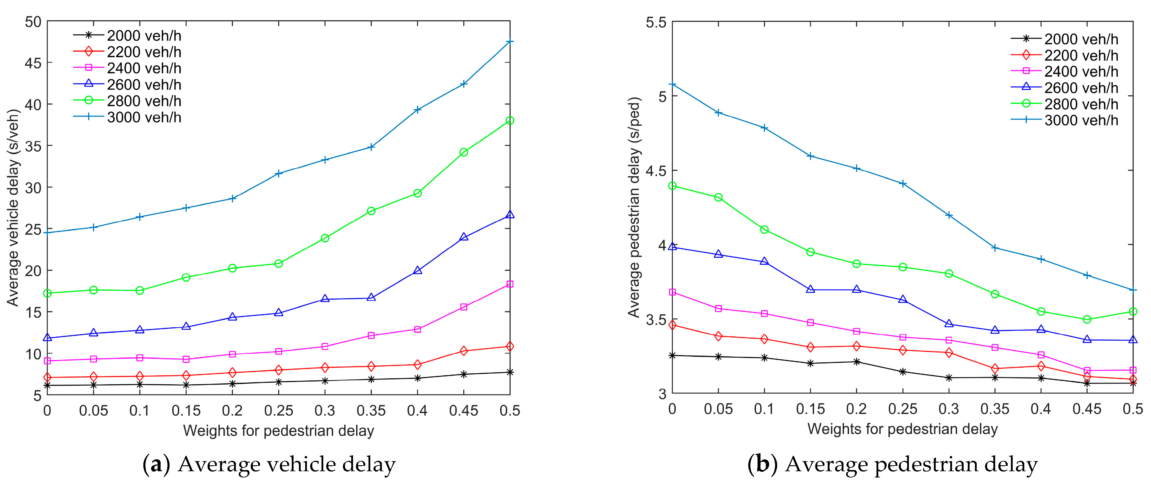
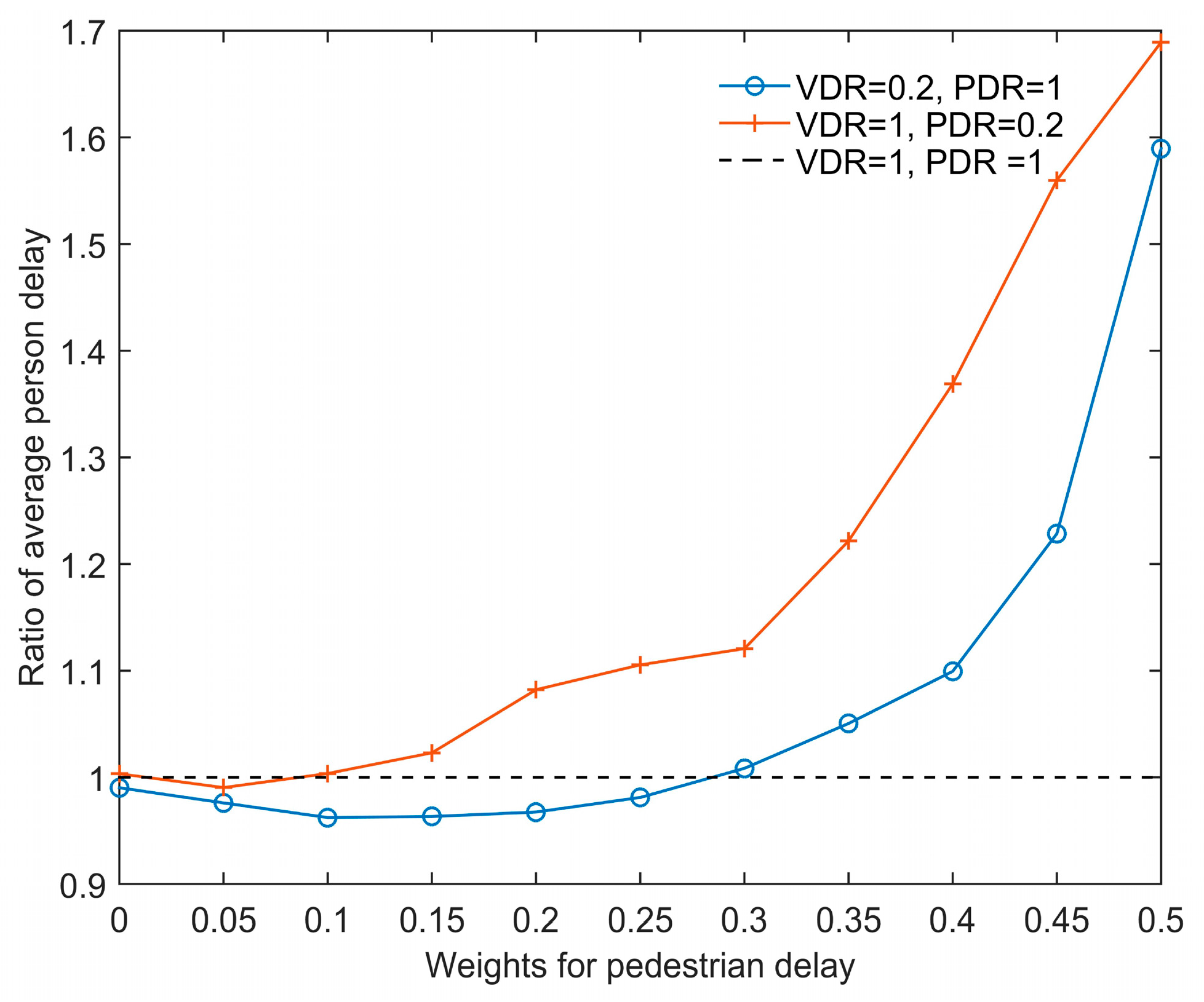
5. Algorithm and Model Analysis

In Table 3, we show the ACS accuracy in comparison to an optimal solution obtained with a full enumeration method and the computation time of both methods. The accuracy is computed based on the average vehicle delay, and the computation time refers to the maximum one across all experiments with 3000 veh/h and 3200 ped/h (if not stated, the tested demands are balanced at the intersection). In order to obtain the optimal solution with the enumeration within reasonable computation time, we set an upper limit of 20 for the total number of vehicles at the intersection (i.e., the first 20 vehicle arrivals within the zone of interest) whose departure sequence is optimized in each decision step. Notice that the ACS algorithm can efficiently solve the problem with a far larger number of vehicles. Table 3 shows the performance of the algorithm when using different settings for the number of ants n ant and the number of iterations n iter . In the ACS algorithm, each ant can find a path (i.e., solution) per iteration. Increasing the number of ants n ant from 10 to 15 can improve the accuracy, as more ants can find more feasible paths (i.e., vehicle departure sequences) and, more likely, find a better solution. Similarly, increasing the number of iterations n iter from 10 to 20 to 30 also increases the accuracy due to the increasing number of feasible solutions. We use the notation CS = (rinfo, rauto) to represent CAV penetration rates, and we test CS = (1.0, 1.0) and CS = (0.5, 0.5) representing the full AVs and a lower CAV penetration rate, respectively.
In Table 3, ACS performs relatively better for CS = (0.5, 0.5) than for CS = (1.0, 1.0) when comparing it to the benchmark method, i.e., enumeration method with these two scenarios. This happens because fewer CAVs lead to computing fewer combinations of vehicle departure sequences, i.e., a smaller solution space, which makes it easier for ACS to reach the optimal solution. In terms of computational time, not surprisingly, increasing the number of ants and iterations increases the cost of ACS. Furthermore, CS = (1.0, 1.0) is computationally more expensive than CS = (0.5, 0.5). This makes sense, as more combinations of vehicle departure sequences are evaluated for CS = (1.0, 1.0). Out of all tested scenarios, the longest computational time is 6.1 s, which was obtained with 15 ants and 30 iterations in the CS = (1.0, 1.0). Notice that a better solution can counterbalance a higher computational time due to a smaller number of vehicles simulated in the zone of interest, even if tests are done with more ants and iterations. Compared to the enumeration method, the ACS can reduce the computational time by a factor of 37–55 while keeping an accuracy >98.5% with n ant = 15, n iter = 30. Although not comparable with the enumeration method because of the reasons explained before, here, we also investigate the ACS algorithm for the case that all vehicles are optimized in each decision step, rather than just 20. In that case, the reductions in average vehicle delay can reach up to 9.4% with CS = (1.0, 1.0) and 1.8% with CS = (0.5, 0.5), compared to the solutions of the enumeration method with an upper limit of 20 vehicles. Such improvements only cost a maximum of 2.4 s of additional time for all the cases compared (see the total computational time within parentheses in Table 3). Moreover, the savings in computational time for the ACS algorithm should be expected to increase in more complicated cases, where the enumeration solution is simply infeasible. According to these results for the analysis that follows, we chose 10 ants and 30 iterations, as well as an optimization that considers all vehicles.
In Figure 5, we show the relationship between the predicted delay in the model optimization and the actual delay observed in the simulation across all tests with 2000 veh/h and 3200 ped/h, full AV penetration rate, and ω = 0. The delay error represented by one dot is the cumulative vehicle or pedestrian delay in one vehicle departure sequence. Notice that we only compare the predicted delay with the actual delay for identical vehicle departure sequences, i.e., the sequence generated by the algorithm and that observed in the simulation need to be the same. As the graph shows, the predicted vehicle delay is close to the observed vehicle delay (see Figure 5a). The small noises are caused by the different car-following models in the control algorithm and in the simulation. Another reason includes changes in the trajectories of the vehicles. The trajectory design in the model guarantees a solution only for one decision step. In future decision steps, the trajectories can be revised on the basis of the updated traffic information. In the case of pedestrian delay (see Figure 5b), the variation is relatively larger. There are two reasons for this. First, while vehicle delay is computed only for the actual vehicles that enter the zone of interest, the pedestrian delay is calculated forecasting a pedestrian arrival rate; such a forecast also includes an error of its own. Second, the predicted pedestrians are assumed to arrive with a uniform process, while the real pedestrian arrivals follow a Poisson process. Although it is also possible to implement a Poisson arrival within the pedestrian delay model (Equation (7)), such a modification will render the problem more complicated, without significantly improving the final solution. With the current model, the pedestrian delays are slightly overestimated when they are short. Nevertheless, the errors are within an acceptable range. According to the comparison with the enumeration method (see Table 3), as well as the validation results (see Figure 5), the ACS algorithm can significantly improve the computation efficiency while ensuring control performance. On this basis, in the next section, we show the ACS control performance with different traffic and pedestrian scenarios in comparison with the benchmark, i.e., an actuated control method.

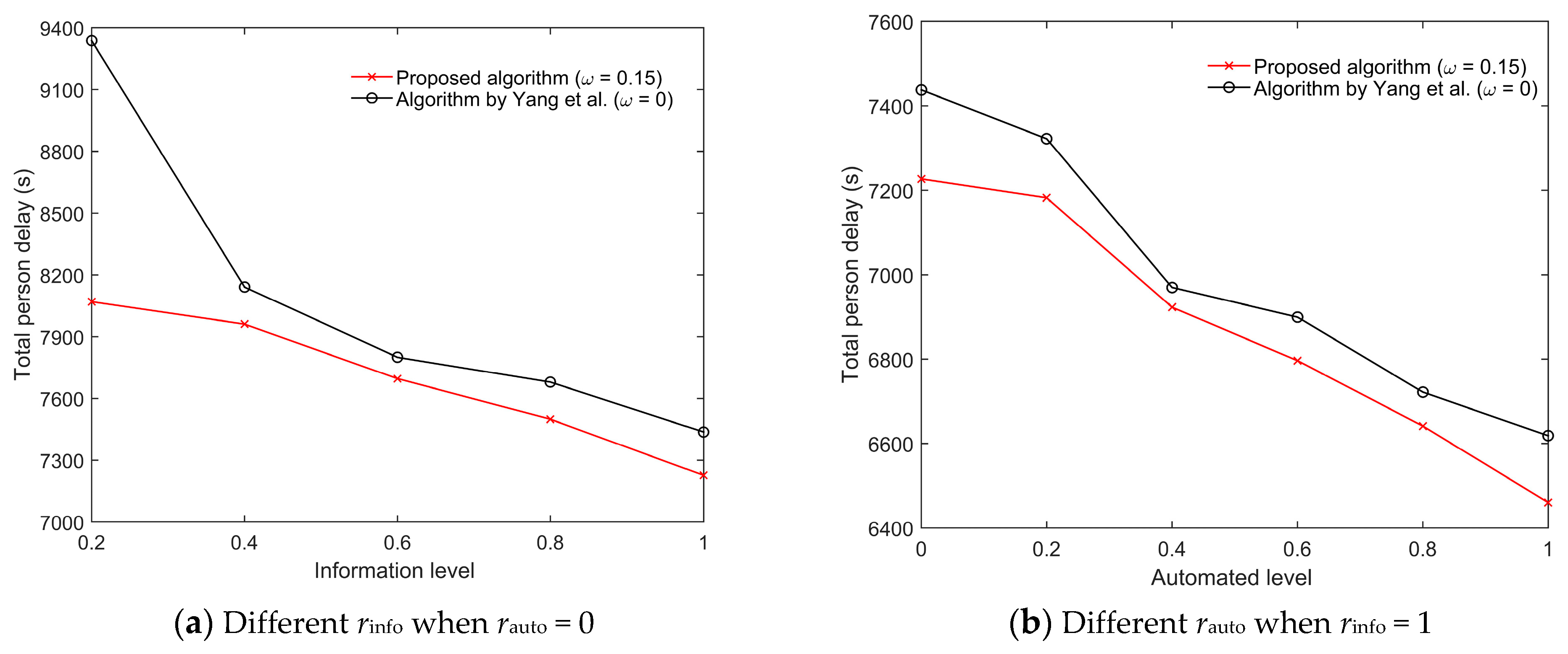
6. Performance of the Control Algorithm

In Figure 6, we compare the proposed algorithm with the actuated control method for different weights of pedestrian delay. To that end, we plot the average person delay obtained with the proposed algorithm divided by that obtained with the actuated control method. A ratio smaller than 1 means that the proposed algorithm outperforms the actuated control method. In the simulation, full AV penetration is tested, and both vehicle demand and pedestrian demand are balanced at the intersection. ω = 0.15 delivers the best solutions for low vehicle demands between 2000 veh/h and 2400 veh/h (the volume to capacity at the intersection ranges from 0.66 to 0.98, according to the tested vehicle demands between 2000 veh/h and 3000 veh/h). The ratios of the best solutions fall in the range of 0.54–0.56. Correspondingly, the proposed algorithm reduces the average person delay by 44–46% compared to the actuated control method. For the low vehicle demands, the proposed algorithm including pedestrian delay (i.e., ω = 0.15) slightly reduces the average person delay compared to a case not including pedestrian delay (i.e., ω = 0). Recall that, when ω = 0, Equation (1) becomes the same optimization as in [19], although the result is obtained with a different solution method (ACS in this paper) and an updated triggering mechanism that also accounts for pedestrian events. For the high vehicle demands (between 2600 veh/h and 3000 veh/h), the best solutions are obtained with ω = 0. In other words, including the pedestrian delay degrades the performance of the algorithm for such high demands. With the optimal weight ω = 0, nevertheless, the average person delays are reduced by 18–42% in comparison to the actuated control.
To further analyze this, in Figure 7, we illustrate the evolution of the average vehicle delay and the average pedestrian delay with the proposed algorithm. With the increasing weights, the average vehicle delay increases (see Figure 7a). Simultaneously, the average pedestrian delay decreases (see Figure 7b). By introducing pedestrians into the optimization, the proposed algorithm offers a clear benefit for pedestrians. However, this comes at the expense of the vehicles, whose delay increases much faster than any reductions for the pedestrians. This is exacerbated in the high-vehicle-demand scenarios. Notice that, in the complete absence of pedestrian priority (i.e., ω = 0), pedestrians will have to wait at most one cycle. On the other hand, giving them priority (i.e., ω ≠ 0) might penalize vehicles disproportionately as they would likely have to wait much longer with the delay lingering for multiple cycles. In other words, while the benefits given to pedestrians are bounded (to at most one cycle), the cost imposed to vehicles is unbounded and can increase significantly in the case of high vehicle demands.
Again, the results in Figure 7 indicate that it is better to include pedestrian delay with small weights into the joint optimization for the low-vehicle-demand scenarios (i.e., 2000–2400 veh/h). By introducing pedestrians into the algorithm, e.g., going from ω = 0 to ω = 0.15, the average pedestrian delay decreases by 6.8%, while the average vehicle delay just increases by 3.3%. Increasing the weight over 0.15 has a diminishing rate of return for pedestrians and might cause a very high cost for vehicles.
The impacts of the unbalanced vehicle and pedestrian demands on the performance of the controller were also investigated. We tested the simulations with the demands of 2400 veh/h and 3200 ped/h. The lowest average person delay with the optimal weight ω = 0.15 under the balanced demands (i.e., VDR = 1, PDR = 1) was set as a reference. As shown in Figure 8, the solutions of the unbalanced vehicle demand (i.e., VDR = 0.2, PDR = 1) are better than the reference case when using weights between 0 and 0.25, and the optimal one remains ω = 0.15. Regarding the unbalanced pedestrian demand (i.e., VDR = 1, PDR = 0.2), we focus on the results that are associated with the proper range of weights from 0 to 0.1. With such weights, the performance is mostly the same as the reference. More precisely, the optimal weight changes to 0.05. The above results show that the unbalanced vehicle demand does not affect the selection of the proper weight ω , while the unbalanced pedestrian demand does have some impact on the weight, which should be adjusted accordingly.
Figure 9 shows the performance of the proposed algorithm under different levels of CAV penetration rates. The balanced demands of 2400 veh/h and 3200 ped/h are implemented with the proposed algorithm using the best weight ω = 0.15. We first investigate the information level rinfo (i.e., the ratio of the number of CAVs to the total number of vehicles) from 0.2 to 1, using an automated level rauto = 0. The rinfo begins from 0.2 rather than 0, as we assume that traffic information is collected only from CAVs. By raising rinfo from 0.2 to 1 (see Figure 9a), the total person delay declines to 7250 s. This represents a 10% improvement. We then look at the impacts on the performance from different rauto. The AV penetration ratio is set from 0 to 1 assuming all vehicles are connected, i.e., rinfo = 1. As a result, the average person delay decreases consecutively from 7250 s to 6450 s, an 11% improvement (see Figure 9b). This shows the value of the AV trajectory planning. More importantly, the new algorithm outperforms that proposed in [19] in all scenarios.

7. Conclusions

This study proposed a control strategy for the joint optimization of vehicle departure sequence, pedestrian crossing, and automated vehicle trajectory at an isolated intersection. The main contributions include (1) proposing a pedestrian delay model to estimate the pedestrian delay during a varying estimation horizon, according to the triggering events and the vehicle departure sequences, (2) clarifying the benefits of CAVs with increases of the penetration rates in relation to pedestrian crossing at the intersection, and (3) developing an ant colony system algorithm to find a near optimal solution with high computational efficiency.
We conducted multiple simulations to ensure the feasibility of the ant colony algorithm and the reliability of the vehicle and pedestrian delay models, as well as to evaluate the control performance of the proposed algorithm. The simulation results show that the proposed algorithm considering pedestrians with the proper weight for pedestrian delay (e.g., ω = 0.15) is always better than the actuated control algorithm and is superior to the CAV algorithm without any weighted pedestrian delay (i.e., no pedestrian priority) in the low- and moderate-vehicle-demand scenarios. Specifically, introducing pedestrians into the signal control algorithm under a CAV environment reduces the average person delay and has a clear benefit for pedestrian delay reduction. Moreover, the total person delay can be reduced even further by increasing the CAV penetration rates.
Caution must be exercised, however, with the selection of the weight for pedestrian delay. If too much weight is given to pedestrians, the algorithm deteriorates quickly and ends up with a worse performance than the actuated traffic controller. This is mainly caused by the unsatisfactory vehicle departure sequences and AV trajectory planning, which are sensitive to the interference of pedestrians with the setting of large weights for pedestrian delay, especially for the high vehicle demands. One way to improve the robustness of the algorithm would be to prolong the decision interval in the optimization. This could also address the problem of computational burden due to highly frequent triggering events when applied to a complex intersection.
Recently, connected pedestrians have attracted increasing attention in the research community. At signalized intersections, connected pedestrians can use a smartphone application to request a pedestrian green to cross the street [43]. Related studies mostly evaluated the conflicts of connected pedestrians and CAVs in terms of safety, instead of operational efficiency. Our proposed algorithm can readily take the requests from connected pedestrians by replacing the action of pedestrians pushing the button. This would give us even better accuracy than the estimations used for pedestrian arrivals. However, such information would not change the insights presented here. We find that, in terms of intersection efficiency, accounting for pedestrian crossing is only valuable for lower traffic demands. For people who take e-bikes, e-scooters, and similar types of micromobility vehicles to pass the crosswalk, they usually have higher speeds than pedestrians. Therefore, their inclusion does not change the pedestrian signal settings in the model, as the minimum pedestrian crossing time should be dictated by the slowest mode.
In this study, we look at a relatively simple case of traffic at the intersection to understand the inclusion of pedestrian crossings for intersection control. Not surprisingly, we find that accounting for pedestrian crossing for intersection control efficiency is only valuable for lower traffic demands even under a CAV environment. Accordingly, future research could focus on fine-tuning the control algorithm using low vehicle demands in more complex scenarios including intersections with turning traffic to investigate the evolutions of related vehicle and pedestrian delays.

Author Contributions

Conceptualization, M.M. and B.Y.; methodology, B.Y., K.Y., and M.M.; software, K.Y. and B.Y.; validation, B.Y., K.Y., and M.M.; formal analysis, B.Y., M.M., and K.Y.; writing—original draft preparation, B.Y.; writing—review and editing, M.M., B.Y., and K.Y.; visualization, B.Y.; supervision, M.M. All authors have read and agreed to the published version of the manuscript.

Funding

This research received no external funding.

Institutional Review Board Statement

Not applicable.

Informed Consent Statement

Not applicable.

Data Availability Statement

Not applicable.

Acknowledgments

This work was partially supported by the NYUAD Center for Interacting Urban Networks (CITIES), funded by Tamkeen under the NYUAD Research Institute Award CG001 and by the Swiss Re Institute under the Quantum Cities™ initiative.

Conflicts of Interest

The authors declare no conflict of interest.

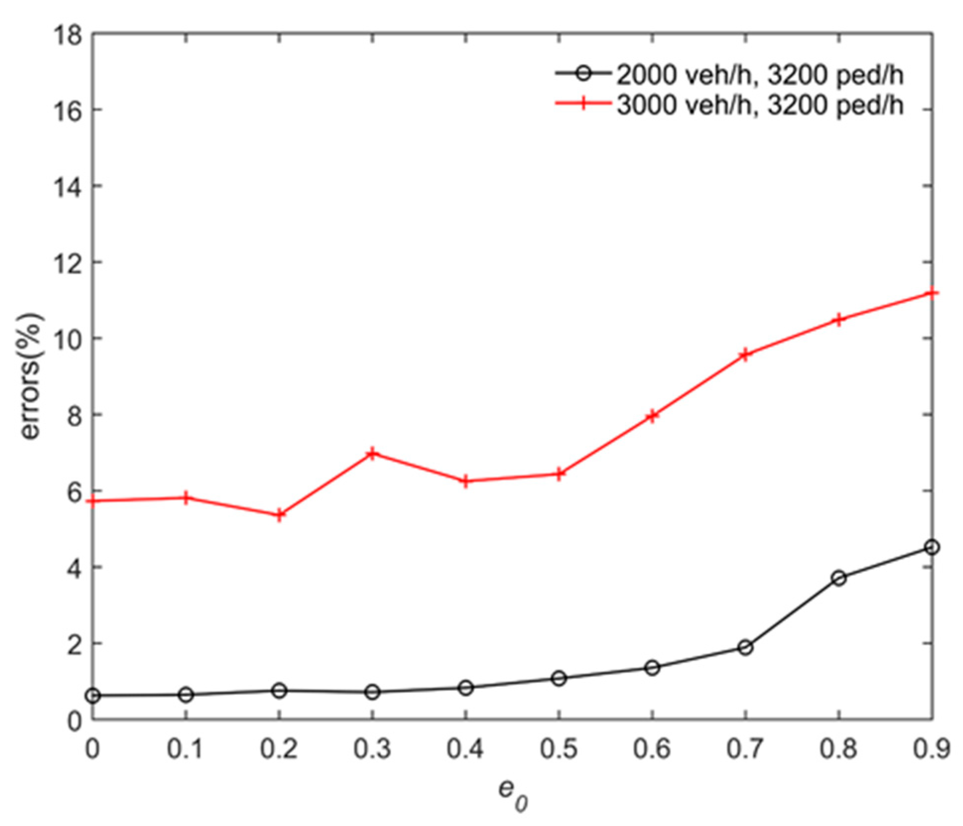
Appendix A. Analysis of the Parameters in ACS Algorithm

For the parameter analysis of the ACS algorithm, two full AV scenarios were tested with vehicle demands of 2000 veh/h and 3000 veh/h, as well as the same pedestrian demand of 3200 ped/h. The tests were carried out using 10 random seeds of the demands with 10 runs per seed. We calculated the average errors between the solutions obtained by the ACS algorithm with specific parameter settings and the optimal solutions obtained by the enumeration method. Notice that we only investigated the solution of the vehicle delay optimization (i.e., ω = 0), and the pedestrian delay optimization was not included in the numerical tests. Potentially, an in-depth sensitivity analysis could be conducted to better estimate the effects of these parameters (as in [44]) including their interaction effects if any (see [45]).
Here, the parameters were initially set with α = 0.1, β = 2, ρ = 0.1, and n ant = 10, according to the report in [39]. In addition, we conservatively set n iter = 20. The procedure for the parameters confirmation in the ACS algorithm is introduced below.
First, we investigated the changes in errors with various e0, as shown in Figure A1. The smaller value of e0 (between 0 and 0.2) gave better results; thus, we adopted e0 = 0.2.
Figure A1. Analysis of the parameter e0.
Sustainability 13 01135 g0a1
Then, we tested the parameters α and ρ together for each scenario. The results for the two scenarios are shown in Table A1a,b, respectively. After comparing the results, we chose the combination of α = 0.1 and ρ = 0.1.
Table A1. Analysis of the parameters α and ρ.
(a) 2000 veh/h and 3200 ped/h
α\ρ00.10.20.30.40.50.60.70.80.9
00.71210.74880.67970.71250.68550.65000.67890.68000.67980.7486
0.11.55310.71760.65470.67940.68830.74530.68810.65980.71450.6786
0.22.52340.83250.72870.68200.63200.71640.68510.68870.68190.7159
0.32.26350.92860.84030.82970.67880.72200.69810.74630.74960.6891
0.42.59911.03040.67020.77020.81160.75560.67910.64640.67870.7094
0.53.02221.77050.80520.73350.67920.67880.67920.74980.75190.6834
0.63.03931.45311.05290.84840.78500.72250.64740.80440.68230.6791
0.73.02731.47900.92120.68660.89210.67590.85410.78310.65910.6789
0.83.11711.65041.09620.75010.71170.64370.75530.67990.71240.6848
0.92.76332.14101.16330.84320.78160.88330.73400.74990.68070.7751
(b) 3000 veh/h and 3200 ped/h
α\ρ00.10.20.30.40.50.60.70.80.9
012.990710.393511.640011.923910.290310.717111.982711.328213.078812.0050
0.18.44335.04155.97147.35247.90878.51928.38408.34128.95818.6485
0.29.83326.13746.79416.87325.80846.34237.48278.52208.55618.2074
0.310.75297.66245.51615.20735.84916.51326.89536.82587.51346.9751
0.411.62957.12616.29076.53726.01456.82606.84936.50428.22127.4090
0.511.93998.40346.55555.72336.02606.55816.18326.56947.64057.7624
0.611.43319.08946.84175.80836.20126.25736.85107.50586.60337.4749
0.711.31568.39697.49517.42556.79066.45045.66157.19688.57319.1214
0.810.13849.15165.81456.62426.02106.47466.27776.70046.18517.1229
0.913.32769.60238.78686.90826.41026.12378.01156.41538.49317.8232
Afterward, we looked for the parameter β. Through the tests, the setting of β = 2 gave the best results in these two scenarios, as shown in Figure A2.
Figure A2. Analysis of the parameter β.
Sustainability 13 01135 g0a2
At last, we tested the number of ants n ant and the number of iterations n iter . Finally, n ant = 10 and n iter = 30 were confirmed as the parameters that provide a satisfactory accuracy with the proper computational time (see Table 3).
From the above tests, the parameters of the ACS algorithm implemented in the study were as follows: α = 0.1, β = 2, ρ = 0.1, e0 = 0.2, n ant = 10, and n iter = 30.

References

  1. National Traffic Signal Report Card, National Transportation Operations Coalition. Available online: https://transportationops.org/publications/2012-national-traffic-signal-report-card (accessed on 1 December 2020).
  2. Lee, J.; Park, B. Development and Evaluation of a Cooperative Vehicle Intersection Control Algorithm Under the Connected Vehicles Environment. IEEE Trans. Intell. Transp. Syst. 2012, 13, 81–90. [Google Scholar] [CrossRef]
  3. Guler, S.I.; Menendez, M.; Meier, L. Using Connected Vehicle Technology to Improve the Efficiency of Intersections. Transp. Res. Part C Emerg. Technol. 2014, 46, 121–131. [Google Scholar] [CrossRef]
  4. Li, L.; Wang, F.Y. Cooperative Driving at Blind Crossings Using Intervehicle Communication. IEEE Trans. Veh. Technol. 2006, 55, 1712–1724. [Google Scholar] [CrossRef]
  5. Lin, D.C.; Jabari, S.E. Transferable Utility Games Based Intersection Control for Connected Vehicles. In Proceedings of the EEE Intelligent Transportation Systems Conference, Auckland, New Zealand, 27–30 October 2019; pp. 3496–3501. [Google Scholar]
  6. Yang, K.; Menendez, M. Queue Estimation in a Connected Vehicle Environment: A Convex Approach. IEEE Trans. Intell. Transp. Syst. 2019, 20, 2480–2496. [Google Scholar] [CrossRef] [Green Version]
  7. Li, L.; Jabari, S.E. Position Weighted Backpressure Intersection Control for Urban Networks. Transp. Res. Part B Methodol. 2019, 128, 435–461. [Google Scholar] [CrossRef] [Green Version]
  8. Maslekar, N.; Mouzna, J.; Boussedjra, M.; Labiod, H. CATS: An Adaptive Traffic Signal System Based on Car-to-Car Communication. J. Netw. Comput. Appl. 2013, 36, 1308–1315. [Google Scholar] [CrossRef]
  9. Yang, K.; Menendez, M.; Guler, S.I. Implementing Transit Signal Priority in a Connected Vehicle Environment with and without Bus Stops. Transp. B Transp. Dyn. 2019, 7, 423–445. [Google Scholar] [CrossRef]
  10. Yang, K.; Zheng, N.; Menendez, M. Multi-scale Perimeter Control Approach in a Connected-Vehicle Environment. Transp. Res. Part C Emerg. Technol. 2018, 94, 32–49. [Google Scholar] [CrossRef] [Green Version]
  11. Pandit, K.; Ghosal, D.; Zhang, H.M.; Chuah, C.-N. Adaptive Traffic Signal Control With Vehicular Ad hoc Networks. IEEE Trans. Veh. Technol. 2013, 62, 1459–1471. [Google Scholar] [CrossRef] [Green Version]
  12. Au, T.C.; Stone, P. Motion Planning Algorithms for Autonomous Intersection Management. In Proceedings of the the 1st AAAI Conference on Bridging the Gap Between Task and Motion Planning, Atlanta, GA, USA, 11 July 2010; Volume WS-10-01, pp. 2–9. [Google Scholar]
  13. Dresner, K.; Stone, P. A Multiagent Approach to Autonomous Intersection Management. J. Artif. Intell. 2008, 31, 591–656. [Google Scholar] [CrossRef] [Green Version]
  14. Kamal, M.A.S.; Imura, J.I.; Hayakawa, T.; Ohata, A.; Aihara, K. A Vehicle-intersection Coordination Scheme for Smooth Flows of Traffic without Using Traffic Lights. IEEE Trans. Intell. Transp. Syst. 2015, 16, 1136–1147. [Google Scholar] [CrossRef]
  15. Ghaffarian, H.; Fathy, M.; Soryani, M. Vehicular Ad Hoc Networks Enabled Traffic Controller for Removing Traffic Lights in Isolated Intersections Based on Integer Linear Programming. IET Intell. Transp. Syst. 2012, 6, 115. [Google Scholar] [CrossRef]
  16. Tachet, R.; Santi, P.; Sobolevsky, S.; Reyes-Castro, L.I.; Frazzoli, E.; Helbing, D.; Ratti, C. Revisiting Street Intersections Using Slot-Based Systems. PLoS ONE 2016, 11, e0149607. [Google Scholar] [CrossRef] [Green Version]
  17. Wu, J.; Abbas-Turki, A.; El Moudni, A. Cooperative driving: An Ant Colony System for Autonomous Intersection Management. Appl. Intell. 2012, 37, 207–222. [Google Scholar] [CrossRef]
  18. Xu, B.; Ban, X.J.; Bian, Y.; Li, W.; Wang, J.; Li, S.E.; Li, K. Cooperative Method of Traffic Signal Optimization and Speed Control of Connected Vehicles at Isolated Intersections. IEEE Trans. Intell. Transp. Syst. 2018, 20, 1390–1403. [Google Scholar] [CrossRef]
  19. Yang, K.; Guler, S.I.; Menendez, M. Isolated Intersection Control for Various Levels of Vehicle Technology: Conventional, Connected, and Automated Vehicles. Transp. Res. Part C Emerg. Technol. 2016, 72, 109–129. [Google Scholar] [CrossRef]
  20. Feng, Y.; Yu, C.; Liu, H.X. Spatiotemporal Intersection Control in a Connected and Automated Vehicle Environment. Transp. Res. Part C Emerg. Technol. 2018, 89, 364–383. [Google Scholar] [CrossRef]
  21. Pourmehrab, M.; Elefteriadou, L.; Ranka, S.; Martin-Gasulla, M. Optimizing Signalized Intersections Performance Under Conventional and Automated Vehicles Traffic. IEEE Trans. Intell. Transp. Syst. 2019, 1–10. [Google Scholar] [CrossRef] [Green Version]
  22. Yu, C.; Feng, Y.; Liu, H.X.; Ma, W.; Yang, X. Integrated Optimization of Traffic Signals and Vehicle Trajectories at Isolated Urban Intersections. Transp. Res. Part B Methodol. 2018, 112, 89–112. [Google Scholar] [CrossRef] [Green Version]
  23. Li, Z.; Elefteriadou, L.; Ranka, S. Signal Control Optimization for Automated Vehicles at Isolated Signalized Intersections. Transp. Res. Part C Emerg. Technol. 2014, 49, 1–18. [Google Scholar] [CrossRef]
  24. Alfonso, J.; Naranjo, J.E.; Menéndez, J.M.; Alonso, A. Vehicular Communications. Intell. Veh. 2018, 15, 103–139. [Google Scholar] [CrossRef]
  25. Carsten, O.M.J.; Sherborne, D.J.; Rothengatter, J.A. Intelligent Traffic Signals for Pedestrians: Evaluation of Trials in Three Countries. Transp. Res. Part C Emerg. Technol. 1998, 6, 213–229. [Google Scholar] [CrossRef]
  26. Ishaque, M.M.; Noland, R.B. Trade-offs between Vehicular and Pedestrian Traffic Using Micro-simulation Methods. Transp. Policy 2007, 14, 124–138. [Google Scholar] [CrossRef]
  27. Li, X.; Sun, J.Q. Effects of Vehicle-Pedestrian Interaction and Speed Limit on Traffic Performance of Intersections. Phys. A Stat. Mech. its Appl. 2016, 460, 335–347. [Google Scholar] [CrossRef]
  28. Schmöcker, J.D.; Ahuja, S.; Bell, M.G.H. Multi-objective Signal Control of Urban Junctions - Framework and a London Case Study. Transp. Res. Part C Emerg. Technol. 2008, 16, 454–470. [Google Scholar] [CrossRef]
  29. Guler, S.I.; Menendez, M. Methodology for Estimating Capacity and Vehicle Delays at Unsignalized Multimodal Intersections. Int. J. Transp. Sci. Technol. 2016, 5, 257–267. [Google Scholar] [CrossRef]
  30. Kothuri, S.; Koonce, P.; Monsere, C.; Reynolds, T. Exploring Thresholds for Timing Strategies on a Pedestrian Active Corridor. In Proceedings of the 94th Annual Meeting of Transportation Research Board, Washington, DC, USA, 11–15 January 2015; p. 16. [Google Scholar]
  31. Li, M.; Alhajyaseen, W.K.M.; Nakamura, H. A Traffic Signal Optimization Strategy Considering Both Vehicular and Pedestrian Flows. In Proceedings of the 89th Annual Meeting of Transportation Research Board, Washington, DC, USA, 10–14 January 2010. [Google Scholar]
  32. Ma, W.; Liao, D.; Liu, Y.; Lo, H.K. Optimization of Pedestrian Phase Patterns and Signal Timings for Isolated Intersection. Transp. Res. Part C Emerg. Technol. 2015, 58, 502–514. [Google Scholar] [CrossRef]
  33. Yu, C.; Ma, W.; Han, K.; Yang, X. Optimization of Vehicle and Pedestrian Signals at Isolated Intersections. Transp. Res. Part B Methodol. 2017, 98, 135–153. [Google Scholar] [CrossRef] [Green Version]
  34. Wray, K.H.; Witwicki, S.J.; Zilberstein, S. Online Decision-making for Scalable Autonomous Systems. IJCAI Int. Jt. Conf. Artif. Intell. 2017, 4768–4774. [Google Scholar] [CrossRef] [Green Version]
  35. Hashimoto, Y.; Gu, Y.; Hsu, L.T.; Iryo-Asano, M.; Kamijo, S. A Probabilistic Model of Pedestrian Crossing Behavior at Signalized Intersections for Connected Vehicles. Transp. Res. Part C Emerg. Technol. 2016, 71, 164–181. [Google Scholar] [CrossRef]
  36. Virkler, M.R. Pedestrian Compliance Effects on Signal Delay. Transp. Res. Rec. 1998, 88–91. [Google Scholar] [CrossRef]
  37. Highway Capacity Manual, Sixth Edition: A Guide for Multimodal Mobility Analysis. Available online: http://www.trb.org/Publications/hcm6e.aspx (accessed on 1 December 2020).
  38. Newell, G.F. A Simplifed Car-following Theory: A Lower Order Model. Transp. Res. Part B Methodol. 2002, 36, 195–205. [Google Scholar] [CrossRef]
  39. Dorigo, M.; Gambardella, L.M. Ant Colony System: A Cooperative Learning Approach to the Traveling Salesman Problem. IEEE Trans. Evol. Comput. 1997, 1, 53–66. [Google Scholar] [CrossRef] [Green Version]
  40. Treiber, M.; Hennecke, A.; Helbing, D. Congested Traffic States In Empirical Observations and Microscopic Simulations. Phys. Rev. E Stat. Phys. Plasmas Fluids Relat. Interdiscip. Top. 2000, 62, 1805–1824. [Google Scholar] [CrossRef] [PubMed] [Green Version]
  41. Yang, K.; Guler, S.I.; Menendez, M. A Signal Control Strategy Using Connected Vehicles and Loop Detector Information. In Proceedings of the 15th Swiss Transport Research Conference, Monte Verità, Ascona, Switzerland, 15–17 April 2015. [Google Scholar]
  42. Dion, F.; Rakha, H.; Zhang, Y. Evaluation of Potential Transit Signal Priority Benefits along a Fixed-time Signalized Arterial. J. Transp. Eng. 2004, 130, 294–303. [Google Scholar] [CrossRef]
  43. Owens, J.M.; Greene-Roesel, R.; Habibovic, A.; Head, L.; Apricio, A. Reducing Conflict Between Vulnerable Road Users and Automated Vehicles. In Lecture Notes in Mobility; Meyer, G., Beiker, S., Eds.; Springer: Berlin/Heidelberg, Germany, 2018; pp. 69–75. [Google Scholar]
  44. Ge, Q.; Ciuffo, B.; Menendez, M. Combining Screening and Metamodel-based Methods: An Efficient Sequential Approach for the Sensitivity Analysis of Model Outputs. Reliab. Eng. Syst. Saf. 2015, 134, 334–344. [Google Scholar] [CrossRef]
  45. Ge, Q.; Menendez, M. Extending Morris Method for Qualitative Global Sensitivity Analysis of Models with Dependent Inputs. Reliab. Eng. Syst. Saf. 2017, 162, 28–39. [Google Scholar] [CrossRef]
Figure 1. A symbolic four-legged intersection.
Sustainability 13 01135 g001
Figure 2. Model framework.
Sustainability 13 01135 g002
Figure 3. Illustration of pedestrian delay model. (ac) All cases to estimate t J end , the ending time of the estimation horizon of pedestrian delay for vehicle departure sequence J. In all cases, we consider n W , the number of signal changes to “walk” for the reference approach starting from the vehicle or pedestrian event time t e and lasting until the last vehicle departure time D | N | , J . We also consider the times of D | N | , J . In (a), n W = 0 , and the upper bound of D | N | , J is the ending time of “flashing do not walk”. In (b), n W = 0 , and the lower bound of D | N | , J is t G , the start time of vehicle green signal on the reference approach after t e . In (c), n W 1 , and the lower bound of D | N | , J is t W = 1 , the start time of W for the reference approach after t e . (d) An example of the pedestrian delay calculated with the triangular areas from t e to t J end on the two conflicting approaches with pedestrian arrival rate λ .
Sustainability 13 01135 g003
Figure 4. Flowchart of ACS algorithm for solution.
Sustainability 13 01135 g004
Figure 5. Relationship between the predicted vehicle or pedestrian delay and the actual vehicle or pedestrian delay.
Sustainability 13 01135 g005
Figure 6. Performance of average person delay with different weights for the pedestrian delay in the joint optimization.
Sustainability 13 01135 g006
Figure 7. (a) Average vehicle delay and (b) average pedestrian delay using the proposed approach with ACS.
Sustainability 13 01135 g007
Figure 8. Comparison of the average person delay between the balanced demand and the unbalanced demand.
Sustainability 13 01135 g008
Figure 9. Performance of the proposed algorithm under different connected and automated vehicle (CAV) penetration rates: (a) different rinfo when rauto = 0, and (b) different rauto when rinfo = 1.
Sustainability 13 01135 g009
Table 1. Notation and parameters. ACS, ant colony system; AV, automated vehicle.
Vehicle delay modelJvehicle departure sequence
Ncurrent vehicle set at each decision step, cars indexed by c (node in ACS algorithm)
smvehicle saturation flow rate for approach m
qmvehicle flow rate for approach m (veh/h)
u f free-flow speed
u c , J init initial speed of vehicle c when entering the intersection within departure sequence J
Vcvirtual departure time of vehicle c from the downstream end of the intersection
Dc,Jpredicted departure time of vehicle c in departure sequence J from the downstream end of the intersection
Pc,Jdelay penalty, i.e., the time it takes for vehicle c in departure sequence J to cross the intersection zone (based on vehicle’s position within a platoon)
Cc,Jthe start time of the signal phase that discharges vehicle c
rinfoinformation level, i.e., the ratio of all equipped vehicles (including connected vehicles and automated vehicles) to the total number of vehicles
rautoautomation level, i.e., the ratio of automated vehicles to all equipped vehicles
Pedestrian delay modelWwalk
DWdo not walk
FDWflashing do not walk
PCpedestrian clearance
ω weights for pedestrian delay, 0 ω < 1
t e time instant of vehicle or pedestrian event
D | N | , J last vehicle departure time in departure sequence J, N
t J end ending time of the pedestrian delay calculation period for departure sequence J
n W number of pedestrian signal changes to W for a reference approach during time interval [ t e ,   D | N | , J ]
t W = k change time of pedestrian W signal at k th   ( k =   0 ,   1 ,   ,   n W ) cycle for a reference approach during time interval [ t e ,   D | N | , J ]
Δ t FDW duration of FDW interval
Δ t PC duration of pedestrian clearance interval (includes FDW and all-red time)
Δ t W min minimum pedestrian green time (W interval)
t FDW start time of FDW interval for pedestrians on a reference approach when n W = 0
t G start time of the green signal for vehicles on a reference Aapproach when n W = 0
λm,naverage pedestrian flow rate (ped/h) for approach m, sidewalk n
R m , r r-th pedestrian waiting interval in approach m (typically includes FDW and DW)
AV trajectory design u c , J des design speed of vehicle c in departure sequence J
u c , J opt optimal speed of vehicle c in departure sequence J
u c , J init initial speed of vehicle c in departure sequence J when entering intersection
u min minimum speed for trajectory design
uffree-flow speed
Table 2. Parameters in the ACS algorithm.
ParameterDefinition
τ ( c , c ) pheromone deposited by ant a ^ from the previous node c to the current node c
η ( c , c ) heuristic information used by ant a ^ from the previous node c to the current node c
p a ^ ( c , c ) probability for ant a ^ to select the next visit node c based on biased exploration
Ω a ^ ( c ) set of nodes that remain to be visited by ant a ^ positioned on the previous node c
ρ pheromone decay parameter in local pheromone updating rule ( 0 < ρ < 1 )
α pheromone decay parameter in global pheromone updating rule ( 0 < α < 1 )
β parameter for heuristic information ( β > 0 )
e 0 parameter for the exploitation of next vehicle c ( 0 e 0 1 )
L0tour length (or discharge time of all vehicles) of any feasible solution for the initialization in local pheromone updating rule
Lglobaltour length (or discharge time of all vehicles) of so-far best path from the beginning of the iteration in global pheromone updating rule
n ant number of ants in ACS algorithm
n iter number of iterations in ACS algorithm
Table 3. Comparison between ACS algorithm and an optimal control method (based on full enumeration) for different ACS parameter sets.
MethodAccuracyComputation Time 1 (s)
Ant colony system (ACS) ( n ant ,   n iter )CS = (1.0, 1.0)CS = (0.5, 0.5)CS = (1.0, 1.0)CS = (0.5, 0.5)
(10, 10)86.73%96.91%1.9(2.5)1.5(1.6)
(10, 20)95.67%98.75%3.5(4.3)2.8(2.3)
(10, 30)97.97%99.79%4.1(5.8)3.2(3.5)
(15, 10)92.65%98.80%3.5(5.0)2.1(3.1)
(15, 20)96.72%99.99%4.3(6.7)2.9(4.6)
(15, 30)98.52%100%6.1(8.1)3.9(6.3)
Enumeration method-100%100%338.9(-)145.1(-)
1 The time without parentheses refers to the case when we use an upper limit of 20 vehicles in the optimization, and the time within parentheses refers to the case when all vehicles are considered in the optimization. The maximum time is chosen from 20 tested samples.
Publisher’s Note: MDPI stays neutral with regard to jurisdictional claims in published maps and institutional affiliations.

