Standing Crop Biomass and Carbon Content of Mangrove Avicennia marina (Forssk.) Vierh. along the Red Sea Coast of Saudi Arabia

Abstract

A number of Avicennia marina mangrove forests exist along the 1134 km stretch of the Saudi Red Sea coast. Three areas, one in each of the north, centre, and south of the coast, were selected for this investigation into the relationship between total biomass (above-ground, AGB, and below-ground, BGB), and biomass carbon stocks of A. marina, along the nutrient availability (combined with a salinity gradient). To estimate the total biomass stock, this research employed equations formulated through a regression approach. Various population characteristics (tree crown diameter, height, and density) and measurements of carbon (C) in the trees were captured, and other measurements were gathered to represent the environmental properties: electrical conductivity (EC), total dissolved solids (TDS), and total phosphorus (TP) and total nitrogen (TN) levels. With this data from the 21 stands and 7 sites of A. marina covered by the three locations chosen along the coast, it was concluded that a discernible influence is exerted by the concentrations of TP and TN in the sea water and sediments over the population characteristics of this plant. The resulting estimates also demonstrated a steady increase in total biomass and total biomass carbon storage from the mangroves in the north toward the south, with values changing overall from 197.9 to 1188.2 Mg DM ha⁻¹ and from 87.6 to 412.5 Mg C ha⁻¹ respectively. This illustrates that the biomasses held by the southern mangroves are 6 times (total) and 4.7 times (total carbon storage) higher than those in the north.

1. Introduction

As there is an intrinsic link between the condition of these mangroves and climate change, information about their status can serve as a barometer to measure and quantify some of its effects. As defined by the IPCC [1], climate change is a persistent, permanent alteration to climate properties, and they affect all aspects of life on this planet. Human health, infrastructures, and safety can all be influenced by climate change, not just the ecosystems, coastal systems, fire occurrence patterns, and overall availability of potable water and food [2]. Furthermore, climate change can and has resulted in significant transformations in the status of the Earth’s oceans, landmasses, and ice sheets, which may well have substantial long-term side effects on related systems. Levels of carbon dioxide in the atmosphere, a key greenhouse gas that contributes to climate change, increased from 280 to 411 ppmv in the 169 years from 1850 to 2019 [3]. A considerable proportion of all the greenhouse gases from anthropogenic sources is represented by deforestation and the production and subsequent use of fossil fuels. Pendleton et al. [4] estimated in their research that this accounted for around 8–20% of total global emissions.

Soil is an important factor in the provision of ecosystem services [5]. Soils play an intrinsic role in the global carbon cycle, sequestering carbon and regulating greenhouse gases [6]. In 1980, Jenny [7] noted the strong relationship between climate and soil quality. Therefore, climate changes resulting from increased concentrations of greenhouse gases may have negative effects on soil structure and its stored organic carbon content, in addition to obstructing water, carbon, and many other important element cycles, causing adverse effects on plant productivity [8]. The relationship between soil and the different characteristics of mangrove forests in the tropics was studied by Hossain and Nuruddin in 2016, where they indicated that soil properties (such as physico-chemical properties) have an impact on the vegetational structure of mangrove forests [9].

The term used to specifically refer to any carbon dioxide that coastal ocean ecosystems generate or capture from the atmosphere is ‘blue carbon’ [10,11,12]. Mangroves represent a sizeable blue carbon system in coastal oceans, and they play a counter-intuitively large role in the attenuation of greenhouse gases, given their small relative area to tropical forests [12,13,14,15]. Across the globe, the blue carbon stored only by mangroves accounts for 11.7 Pg C, a tremendous quantity for their size. Uniquely positioned, Twilley et al. [15] proposed that it is a combination of their potential nutrient exchange with coastal water, and their straddling of the terrestrial-ocean interface, that results in their high degree of contribution to coastal ocean carbon biogeochemistry.

Other environmental factors positively influenced by mangroves include the augmentation of the marine food web in oligotrophic water in its proximity [16], habitat and nutrition provisions for many aquatic and bird species, coral reef protection, and a number of various physical attributes [17,18,19]. By acting as a nutrient filter, mangroves fulfil crucial roles from other perspectives aside from blue carbon, such as ecological and socioeconomic, as humans can benefit from them in many ways [20]. In addition to the boon of the enhanced marine food web and the various ecological factors, Almahasheer et al. [21] observed in their research that the mangroves functioned as wind, wave, and even hurricane barriers for the local population, and their root systems helped to stave off erosion through sediment stabilisation. As stated previously, proportional to their size, mangroves perform a significant role in the carbon cycle. Despite covering only around 137,600 km² of ground split between 118 countries [22], mangroves’ carbon input into ocean systems makes up 11% of the total terrestrial carbon input [23]. It is for these reasons, Sasmito et al. [24] asserted that, of the whole globe, mangroves are one of the most productive ecosystems currently known. Predominantly comprised of trees and shrubs, this forested wetland can develop into broad swathes, and favours the muddy and carbonate coastal areas of tropical and subtropical regions [25,26].

Given their inherent importance in managing carbon levels and their other environmental contributions, these systems should be observed, studied, and preserved wherever possible; however, mangrove ecosystems are highly threatened [27] and in a state of decline, with a rate worse than the rainforests and coral reefs [28,29]. Forest harvesting and other human actions have resulted in a significant deterioration in mangrove ecosystem numbers, with an estimated 35% of the total global mangrove area destroyed over the past two decades alone [28,29]. Despite harvesting nearly all live biomass, Sasmito et al. [24], in its study on mangroves of West Papua Province, Indonesia, asserted that soil carbon stocks were left relatively undisturbed, while aquaculture conversion withdrew 85% of its live biomass carbon stock and 60% of its soil carbon stock.

The mangrove forests are remarkably resilient; Edwards and Head [30] insisted that they could not possibly thrive in proximity to the Red Sea, given the local environmental conditions. However, in the past 40 years, and possibly because of rejuvenation initiatives, the proliferation rate of mangroves for that area has increased by 12%, such that they now occupy 135 km² of the Red Sea coast [31]. In the eastern and western coastal areas of the Arabian Peninsula, mangroves also thrive [32]. This all has given the mangrove forest a reputation for its capacity to thrive in usually harsh and inhospitable circumstances; many living things struggle in environments with high concentrations of salt, sparse rainfall, dehydrated land, and a complete lack of riverine systems, making the mangrove forests the subject of much attention [33]. A pioneer species, Avicennia marina (Figure S1) stores carbon in both biomass and sediments [27], and paves the way for full mangrove forests to develop in otherwise challenging areas. In many areas of Saudi Arabia, the conditions are inhibitive for these mangrove forests, however, along the Red Sea coast’s intertidal zones, some isolated stands manage to survive, grow, and thrive [32]. Over 48 km² of this coastline is now inhabited by A. marina (Almahasheer, personal communication), and it is particularly more prolific in southern or coastal regions as opposed to inland or northern [34].

Though there was not a substantial amount for arid and semiarid environments, an analysis of the available research revealed a focus on reliably and accurately estimating soil carbon and aboveground biomass [10,21,35,36,37]. Consideration by region allowed some academics to produce estimations for the average values for tropical wet, tropical dry, and subtropical mangroves’ AGB growth rates; at 9.9, 3.3, and 18.1 Mg of dry matter ha⁻¹ year⁻¹ [38,39,40]. However, some authors looking into more specific areas, such as Wang et al. [41], elected to quantify total mangrove AGB in their study instead of its growth rate; giving a value in the northeast of China’s Hainan Island of 312,806.3 Mg. Parvaresh [42] also looked at total instead of rate, however, like many other authors, they accounted for area when they performed their own study into the AGB of A. marina trees in Iran, focusing on those in the arid climate of Sirik. They found the total AGB to be 17.2 Mg ha⁻¹, a value that is comparatively low when considering other similar research. In the Mangawhai Harbour in New Zealand, Tran et al. [43] estimated the ABG of the same species at between 0.3–0.9 Mg ha⁻¹, significantly less than in other similarly temperate zones, both within the same country and Australia. In the same study, they additionally recorded the BGB, which was interestingly in line with that of the larger tree locations, despite less AGB, at a value between 1.2–1.5 Mg ha⁻¹. Although the majority of authors in this field centred their work on AGB, Tamooh [44] in Kenya, in the Gazy Bay, investigated multiple species’ BGB instead, estimating a value of 43 Mg ha⁻¹ for A. marina, while Mackey [45] reported 109–126 Mg ha⁻¹ in Australia for the same species a few years prior.

While there are many papers in other locations worldwide on the status of mangroves, their carbon contents, and estimations of their biomasses, there are not as many specifically in the Arabian region. Two of those that are, include one study in Egypt and one in Saudi Arabia. Mashaly et al. [27] performed their research in the former, estimating total biomass carbon content (in Mg C ha⁻¹) and an average value for single-tree biomass (in kg) for various types of mangroves in South Sinai. Respectively, their reported figures for those were as follows: 109.3 and 92.3 for intertidal mangroves, 41.9 and 16.6 for shoreline mangroves, 70.3 and 40.5 for salt plain mangroves, and 29.2 and 21.2 for transplanted mangroves. Within Saudi Arabia, Abohassan et al. [46] investigated two locations, Shuaiba and Yanbu, along the Red Sea coastline. They estimated both the AGB and BGB for these regions, discovering that the total AGB in Shuaiba was 18.6 Mg ha⁻¹, a substantial 7.8 Mg ha⁻¹ higher than that of Yanbu. They also observed that in addition to having more AGB, Shuaiba also possessed a much greater quantity of aerial and fine roots than Yanbu, with 23.7 and 96.4 Mg ha⁻¹, respectively, for Shuaiba and 10.1 and 39.1 Mg ha⁻¹ for Yanbu.

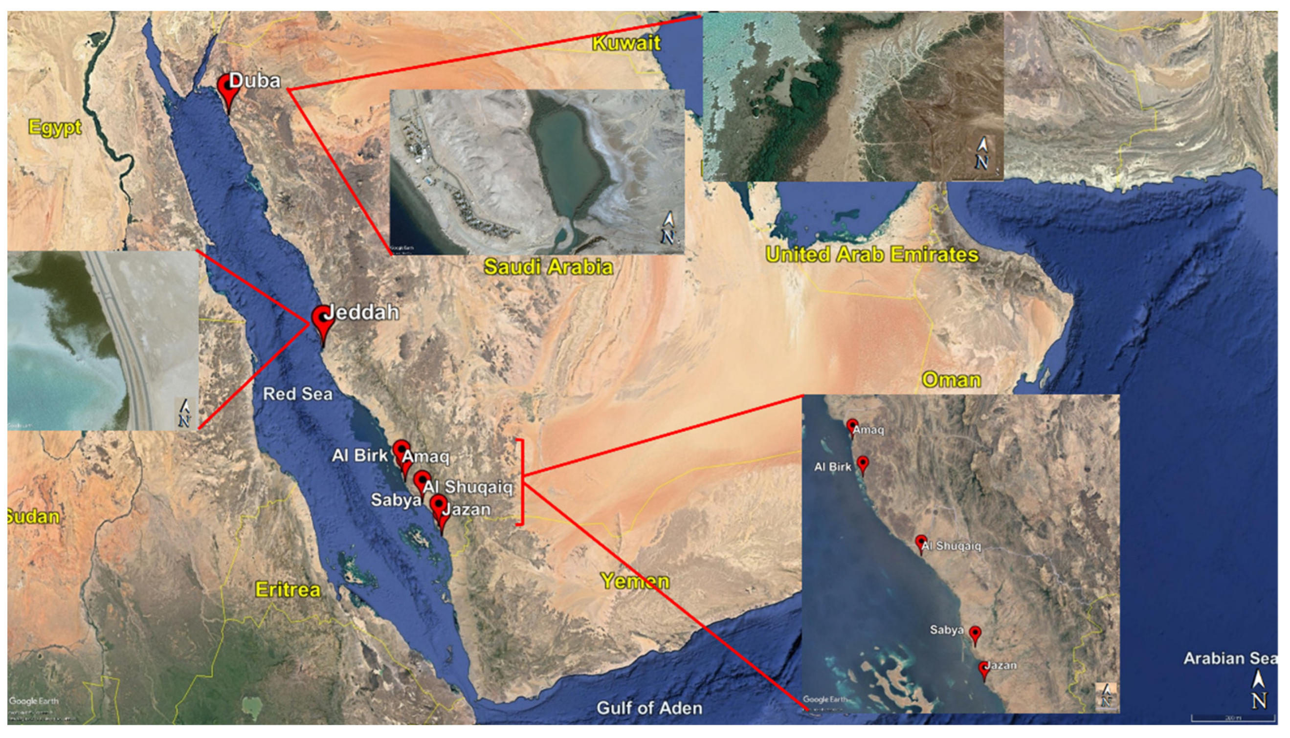
At the time of writing, despite some existing evaluations into the biomass carbon of the mangrove forests for some discrete areas along the Saudi Arabian Red Sea coast, no studies were found to have representatively accounted for the whole of the coastline. From the city of Duba in the north to Jazan in the south, the coast of the Red Sea stretches across around 1134 km of Saudi Arabia, and this study aims to fill the research gap by assessing the AGB and BGB of A. marina mangrove trees along its length. The salinity gradient and nutrient availability in the various locations throughout the coast were likely to affect biomass carbon, and this paper aims to evaluate that influence.

Thus, the objectives of the present study were to (1) evaluate the environmental determinants of the ability of mangroves to capture carbon along the Saudi Red Sea coast; (2) formulate regression equations to anticipate mangrove biomass; and (3) assess the overall tree carbon in mangrove stands of natural occurrence. Some soil management strategies (such as organic cultivation) have a great impact on improving and raising the soil’s organic carbon content, which helps mitigate climate changes resulting from increased concentrations of greenhouse gases [47]. Therefore, the findings of this study are likely to have a broad range of derivative applications for contexts across the globe; possibly assisting in the discovery of new carbon emission reduction and management techniques, such as through the mitigation of mangrove forest or other high-value ecosystem deterioration.

2. Materials and Methods

2.1. Study Area

Nestled with northeast Africa to its west, and the Arabian Peninsula to its east, the slender Red Sea stretches about 2000 km long, down to Bab El-Mandeb (13° N) from the north side of the Suez Gulf (30° N) [32]. A significant 1700 km of its coastline is in Saudi Arabia, intersected by the Tropic of Cancer between Yanbu and Rabegh, making up around 80% of its total length. Despite the constriction of the coastal plain by the mountains beyond [48], as can be seen in Figure 1, the coastal belt’s topography does not significantly differ throughout [49].

Environmentally, the Saudi Red Sea coast does not present optimal conditions for plant growth, with a high salinity (>40 g L⁻¹), hot summer air temperatures (37.5–42.0 °C), low rainfall levels (2.8–22.3 mm year⁻¹), reduced fertility as a result of scarce nutrient supply, lack of freshwater sources, and sandy sediment [21]. Renowned for its highly arid climate, high temperatures, and low rainfall levels [50], Saudi Arabia already presents a challenge to life in the region, even without the added salinity factor. With northerly winds in the winter and southerly winds in the summer [51], most of the limited rainfall for Saudi Arabia’s south-western regions is due to monsoons in the Indian Ocean; a further gradient from north to south is produced by this environment, with substantially greater rainfall in the south [18]. In addition to the environmental factors, many human activities (such as camel and livestock grazing, depositing waste along the beaches and in the sea, and shrimp farming) increase the pressure on the ecosystems here [52,53]. The result of the combination of these factors, as discussed by Shaltout et al. [54], is that the northern region is much less hospitable to plant life than the south. This can be easily discerned, given that in the northern region, the mangrove belt never exceeds 50 m [55], and in some areas is only a single file of trees. Avicennia marina is not the only kind of tree prominent when observing this coastline, and some groups of Rhizophora mucronata Lam. can be found—particularly on the Al-Wajh Bank and the Farasan Islands [16,56]. It is worth noting, however, that in November and January A. marina engages in propagule development and attains its peak flowering stage for the year, characterising the plant clearly [57].

2.2. Sampling Locations

As can be seen in Figure 1, Figure S2 and Table S1, three primary locations on the coastline were selected for sampling, giving seven sites total for the three locations. One northern site with three stands, one central site with three stands, and five southern sites with 15 stands of A. marina mangroves were chosen for analysis in this study, giving 21 stands in total. Though a 736 km stretch of coastline separates the northern and central locations, the southern location is only 398 km from the centre. Comparatively, the northern sample site possessed an extremely low quantity of precipitation, high land dryness, high salinity, and relatively low temperatures [49]. The central location represents an even greater environmental challenge for A. marina mangroves as, while it has similarly limited precipitation, it also suffers from higher temperatures and an extreme climate [58], with the additional element of sewage and fertiliser disposed in the water, causing eutrophication [21]. Conditions in the southern location are comparatively hospitable, with sufficient nutrient availability, greater quantities of precipitation, favourable temperatures, pliable muddy soil, and reduced salinity levels [49].

2.3. Population Characteristics

In order to effectively calculate the population characteristics to reasonable accuracy, the following approach was employed consistently. At each sampling stand, three 10 m × 10 m quadrats of unspecified and random distribution were selected as samples for direct measurement of population tree density, tree crown diameter, and tree height. The latter was captured through use of a measuring tape to interpret the vertical distance from the sediment surface to the maximum canopy point. For the crown diameter, firstly, the same tape was used to measure two perpendicular diameters that crossed at the centre of the canopy and then an average was taken from those values [59].

2.4. Sediment Sampling and Analysis

In the interest of improving result reliability, a consistent method was devised and rigorously followed for the sampling and analysis of the sediment in the research area. Sixty-three sediment samples were gathered—three from each stand—to allow for quantification of the local variables: EC (electrical conductivity), TDS (total dissolved solids), TP (total phosphorus), and TN (total nitrogen). To enable the simple chemical profiling of the samples and therefore the physical locations they represent, first the samples were air-dried and then sieved through a mesh with 2 mm apertures, to remove extraneous debris and gravel particulates, before being hydrated at a ratio of five parts water for one part sediment. Both EC and TDS were measured with a Hanna Instruments conductivity meter (Hanna Instruments, Woonsocket, RI, USA, HI 98130). The sediment preparations were then analysed using the techniques of molybdenum blue [60] and indophenol blue [61] to identify TP and TN at 885 nm and 660 nm wavelengths, respectively, with a spectrophotometer (Perkinelmer, Waltham, MA, USA, Lambda 25).

2.5. Sea Water Sampling and Analysis

Though the water samples collected were brought back to the lab for analysis, for increased accuracy the TDS and EC needed to be measured immediately following the acquisition of a sample, and the nutrient level needed to be stabilised such that it would remain relatively unchanged by the time it reached the lab. To achieve this, three simple 1L polyethylene bottles were used to hold samples taken from the water at low tide, when the water depth was less than 0.3 m. First, the samples EC and TDS values were assessed in the same manner as the sediment preparations; with a conductivity meter (Hanna Instruments, Woonsocket, RI, USA, HI 98130). Next, using Whatman nylon membrane filters (pore size 0.45 mm, diameter 47 mm) the water samples were filtered then, using nitric acid (Analar) to a pH of 2.0, the samples were acidified to stave off nutrient deterioration. Once finally in the lab environment again, the same methods as used for testing TP and TN in sediment preparations was utilised for the water samples.

2.6. Plant Sample Collection and Assessment of Biomass and Carbon of Mangrove Trees

To formulate the regression equations that would be used to assess A. marina mangrove biomass quantities, representative samples needed to be analysed first to give guideline values. For this reason, 48 A. marina plants with stem lengths between 7–130 cm were extracted from the three locations and sent to the laboratory in polyethylene bags. These samples were then subdivided into leaf, stem, and root categories, to differentiate between AGB and BGB, before being dried steadily at 60 °C until their weight ceased to fluctuate. This data combined with the information on height and crown diameter permitted the derivation of regression equations that were used in turn to estimate the biomasses of the mangroves, per m² and then per ha. Circumscribing below the base of A. marina trees to 50 cm, the fine, coarse, and pneumatophore root systems account for the BGB, while the stems, branches, and leaves represent the AGB. Kauffman and Donato’s [62] research provided the global default factors of 0.48 for AGB and 0.39 for BGB, derived from tissue nutrient analysis, and employed in this study to find the level of carbon in the trees.

2.7. Statistical Analysis

For all of the statistical analyses on the data, the SPSS 15.0 software [63] was utilised to assess distribution normality, variance uniformity, and log-transformation, where necessary. As the goal in building the equations that predicted leaf, stem, and root biomass was to be accurate, it was necessary to evaluate the models with respect to their estimates. The Student’s t-test method was used with a validation dataset of another 34 plants, revealing that the chosen equations were in the minimal t-test value. A regression procedure was employed on 48 specimens from the three locations to illustrate any statistical correlation between the AG and BG biomasses, and the tree crown diameter and height. The relationships between the sediment properties, water properties, and the ordination axes; and those linking tree density, height, crown diameter, and total biomass were predicted using the researcher’s calculated Pearson’s simple linear correlation (r) values. Canonical Correspondence Analysis (CCA) was performed using CANOCO 5.0 for Windows [64] to identify the ordination of the population parameters with respect to the nutrient availability and salinity gradients. This was conducted using the tree density, crown diameter, and height as population parameters, and with the sediment and water properties representing the gradients. In identifying any potential statistically significant discrepancies in the chemical and population parameter estimations from the three locations, a one-way analysis of variance (ANOVA) was also carried out. Furthermore, with respect to the research locations averages, it was crucial to implement Tukey’s HSD test to discern discrepancies of importance (p < 0.05). Means followed by different letters are significantly different at p < 0.05 according to Tukey’s HSD test. These letters (a, b, c) indicate the order of the means in ascending order.

3. Results

The sediment and sea water sample results illustrate the environmental conditions at each location, and can be seen in

Table 1. Variation in the sediment characteristics [mean ± standard error] of the three locations supporting Avicennia marina populations along the Red Sea coast of Saudi Arabia.

Location	EC [mS cm−1]	TDS [ppt]	TP [mg 100 g−1]	TN [mg 100 g−1]
Northern	5.27 a ± 0.44	2.63 a ± 0.22	2.10 a ± 0.10	3.30 a ± 0.20
Central	6.45 a ± 0.44	3.23 a ± 0.22	4.80 b ± 0.50	5.20 c ± 0.40
Southern	6.12 a ± 0.75	3.07 a ± 0.38	2.30 a ± 0.20	4.30 b ± 0.20
F-value	0.2 ns	0.2 ns	17.3 ***	8.8 **

F-values represent the one-way ANOVA, **: p < 0.01, ***: p ˂ 0.001, ns: not significant (i.e., p > 0.05), EC: Electrical conductivity, TDS: Total dissolved solids, TP: Total phosphorus, TN: Total nitrogen. Means in the same columns followed by different letters are significantly different at p ˂ 0.05 according to Tukey’s HSD test.

and

Table 2. Variation in the sea water characteristics [mean ± standard error] of the three locations supporting Avicennia marina populations along the Red Sea coast of Saudi Arabia.

Location	EC [mS cm−1]	TDS [ppt]	TP [mg L−1]	TN [mg L−1]
Northern	64.29 a ± 1.34	32.11 b ± 0.67	2.74 a ± 0.60	5.09 a ± 0.26
Central	56.11 a ± 5.54	29.08 ab ± 3.72	11.74 b ± 2.24	10.87 b ± 0.40
Southern	37.35 a ± 5.24	19.11 a ± 2.48	3.71 a ± 0.37	7.08 a ± 0.46
F-value	3.5 ns	3.8 *	26.0 ***	10.3 **

F-values represent the one-way ANOVA, *: p < 0.05, **: p < 0.01, ***: p ˂ 0.001, ns: not significant (i.e., p > 0.05), EC: Electrical conductivity, TDS: Total dissolved solids, TP: Total phosphorus, TN: Total nitrogen. Means in the same columns followed by different letters are significantly different at p ˂ 0.05 according to Tukey’s HSD test.

. EC and TDS values of the sediment samples remained relatively consistent; however, the TP and TN values were vastly dissimilar, lowest in the northern location and highest in the central one (Table 1).

Sea water samples were in accordance with sediment samples for TP and TN, also showing the northern location with the least, and the central with the most (Table 2). However, in contrast to the sediment samples, the EC and TDS values demonstrated a dramatic concentration gradient, this time greatest in the north and smallest in the south.

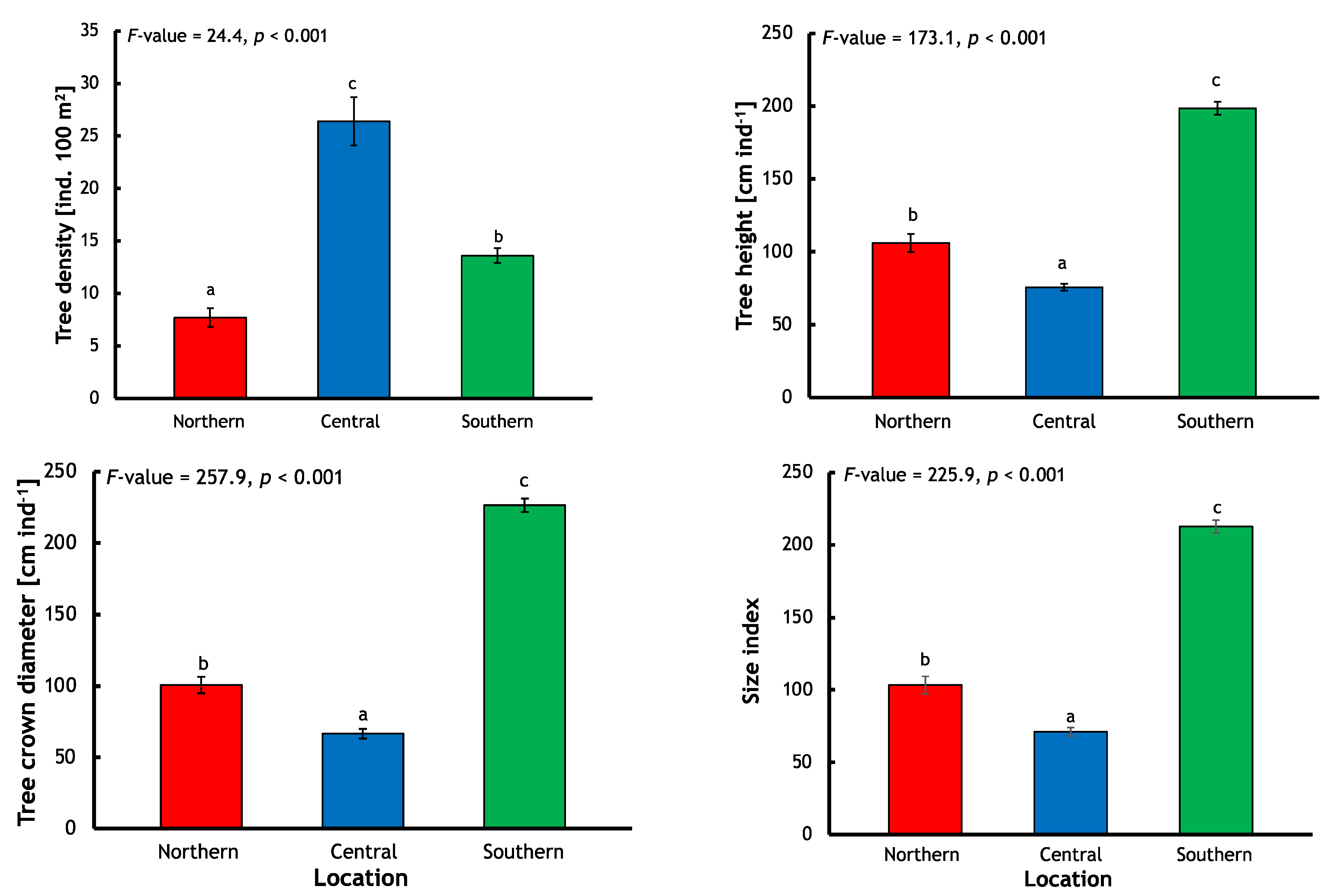
Avicennia marina population characteristics in each location served to elucidate the particular circumstance and condition of the species within those different settings (Figure 2). It was found that while the southern location mangroves had the greatest values for size index (212.6), tree height (198.6 cm ind.⁻¹), and tree crown diameter (226.5 cm ind.⁻¹), they only had a medium tree density (13.6 ind. 100 m²). Contrastingly, despite the central location having the smallest size index (71.7), tree height (75.6 cm ind.⁻¹), and tree crown diameter (66.5 cm ind.⁻¹) properties, it possessed the greatest tree density (26.4 ind. 100 m²) (Figure 2).

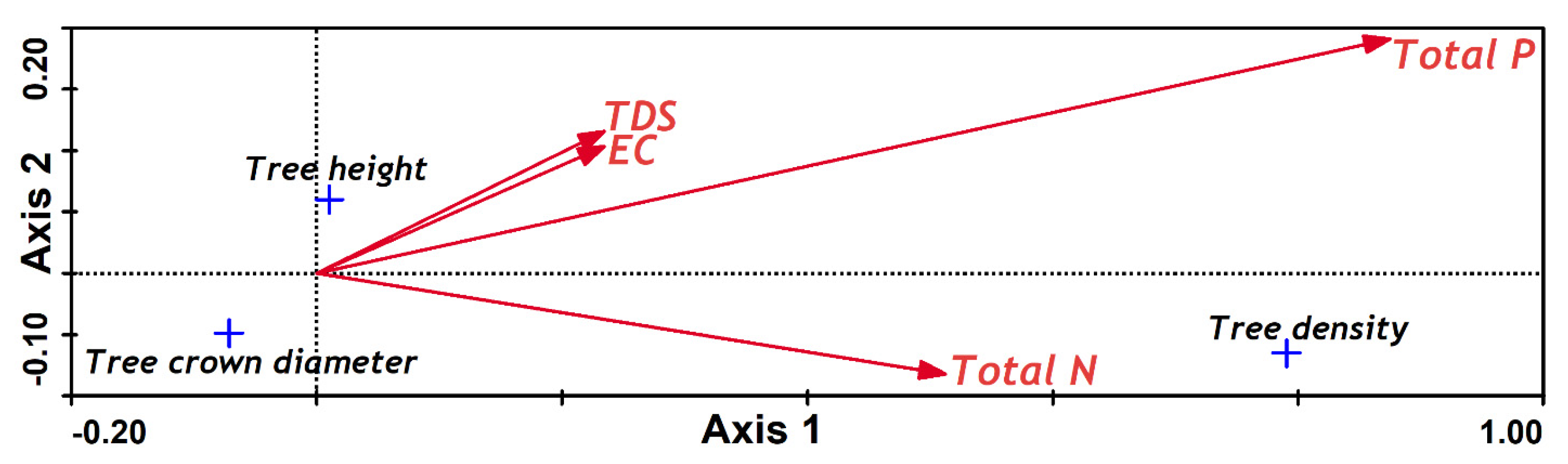
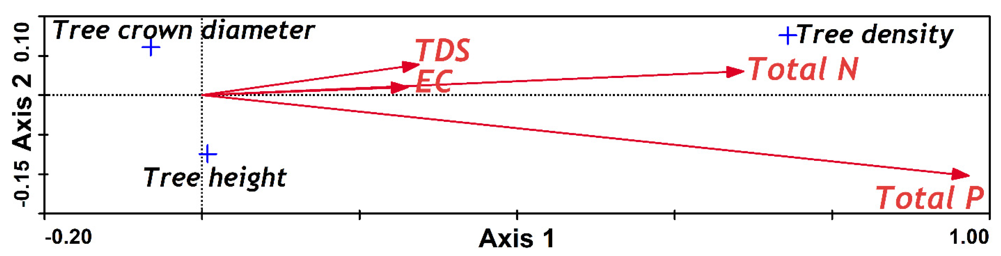
Two CCA were conducted, both between the first two population axes, with one against sediment properties and the other against sea water properties (Figure 3 and Figure 4); TP and TN were found to positively affect the separation of the population characteristics in both analyses. However, for the sediment properties CCA, the second axis was negatively correlated with TN (

Table 3. Inter-set correlations of sediment characteristics with CCA axes.

Sediment Characteristic	Axis 1	Axis 2
Electrical conductivity [mS cm−1]	0.23	0.08
Total dissolved solids [ppt]	0.23	0.09
Total phosphorus [mg 100 g−1]	0.87	0.15
Total nitrogen [mg 100 g−1]	0.51	−0.06

), whereas for water properties, it was negatively correlated with TP (

Table 4. Inter-set correlations of sea water characteristics with CCA axes.

Sea Water Characteristic	Axis 1	Axis 2
Electrical conductivity [mS cm−1]	0.24	0.01
Total dissolved solids [ppt]	0.26	0.04
Total phosphorus [mg L−1]	0.91	−0.10
Total nitrogen [mg L−1]	0.64	0.03

).

The final regression equation employed in the prediction of both AGB and BGB components was most accurate for all seven sites in all three locations when it was plotted linearly, in the form of $y=a+b\left(x\right)$, where $y$ is the biomass, $x$ is the parameter, and both $a$ and $b$ are constants. As briefly touched on in the statistical analysis section of this paper, the Student’s t-test determined a lack of significant difference between actual sample measurements of biomasses and their estimated quantities using the regression equations. Furthermore, the location biomass for both total biomass and each particular biomass component was evaluated, taking advantage of generated prediction models (

Table 5. Variance analysis for regression equations used for predicting the leaves, stems, and roots biomass of Avicennia marina populations along the Red Sea coast of Saudi Arabia.

Equation	R2	Biomass [g DM ind.−1]		t-Value	p
		Actual	Estimated
Northern location
Leaf biomass = [0.570 × D] − 2.001	0.953	5.46	5.48	0.04	0.972
Stem biomass = [1.185 × H] − 30.553	0.465	20.28	20.85	0.06	0.952
Root biomass = [0.058 × H] + [1.054 × D] − 4.806	0.509	11.62	11.55	0.02	0.988
Total biomass = [1.992 × H] − 48.729	0.507	37.36	37.68	0.02	0.982
Central location
Leaf biomass = [1.175 × H] − 32.157	0.657	28.33	28.48	0.02	0.986
Stem biomass = [2.132 × H] − 62.798	0.745	44.74	47.23	0.20	0.843
Root biomass = [1.500 × D] − 4.928	0.868	14.77	14.48	0.18	0.858
Total biomass = [3.703 × H] − 102.185	0.729	87.84	88.92	0.05	0.962
Southern location
Leaf biomass = [2.235 × D] − 19.852	0.743	28.30	26.74	0.29	0.776
Stem biomass = [2.275 × D] − 19.454	0.909	27.46	27.97	0.14	0.893
Root biomass = [1.844 × H] − 59.897	0.526	26.98	25.40	0.16	0.879
Total biomass = [7.388 × D] − 69.375	0.908	82.74	84.63	0.17	0.867

H: Tree height [cm ind.⁻¹], D: Tree crown diameter [cm ind.⁻¹].

).

As can be seen in

Table 6. Above-ground, below-ground and total biomass of Avicennia marina populations along the Red Sea coast of Saudi Arabia.

Location	Biomass [Mg DM ha−1]
	Above-Ground	Below-Ground	Total
Northern	115.5 a ± 26.7	82.4 a ± 16.2	197.9 a ± 42.9
Central	410.0 b ± 54.6	250.9 b ± 26.2	660.9 b ± 78.8
Southern	882.7 c ± 24.8	305.5 b ± 13.6	1188.2 c ± 28.9
F-value	117.5 ***	28.8 ***	119.8 ***

F-values represent the one-way ANOVA, ***: p ˂ 0.001, Mg: 10³ kg. Means in the same columns followed by different letters are significantly different at p ˂ 0.05 according to Tukey’s HSD test.

, there were significant variations in both the calculated biomass levels and proportions of AGB to BGB between locations. In terms of total biomass (Mg DM ha⁻¹), the mangrove in the south possessed the greatest at 1188.2, the central mangrove was almost half that at 660.9, and the north location was only 197.9.

Proportionally, the percentages of total biomass that were above-ground for each location provided further insights; the location in the north had 58.4%, the centre had 62%, and the south had around 75%. Only a quarter of the southern mangrove’s biomass was below-ground. As can be observed in

Table 7. Above-ground, below-ground and total carbon of Avicennia marina populations along the Red Sea coast of Saudi Arabia.

Location	Carbon [Mg C ha−1]
	Above-Ground	Below-Ground	Total
Northern	55.4 a ± 12.8	32.2 a ± 6.3	87.6 a ± 19.1
Central	196.8 b ± 26.2	97.8 b ± 10.2	294.6 b ± 35.6
Southern	288.8 b ± 19.4	123.7 b ± 6.4	412.5 b ± 25.3
F-value	18.1 ***	7.9 **	14.3 ***

F-values represent the one-way ANOVA, **: p ˂ 0.01, ***: p ˂ 0.001, Mg: 10³ kg. Means in the same columns followed by different letters are significantly different at p ˂ 0.05 according to Tukey’s HSD test.

, the total biomass carbon content in Mg C ha⁻¹ for the selected three locations is, in descending order: southern, 412.5; central, 294.6; and northern, with the least, 87.6.

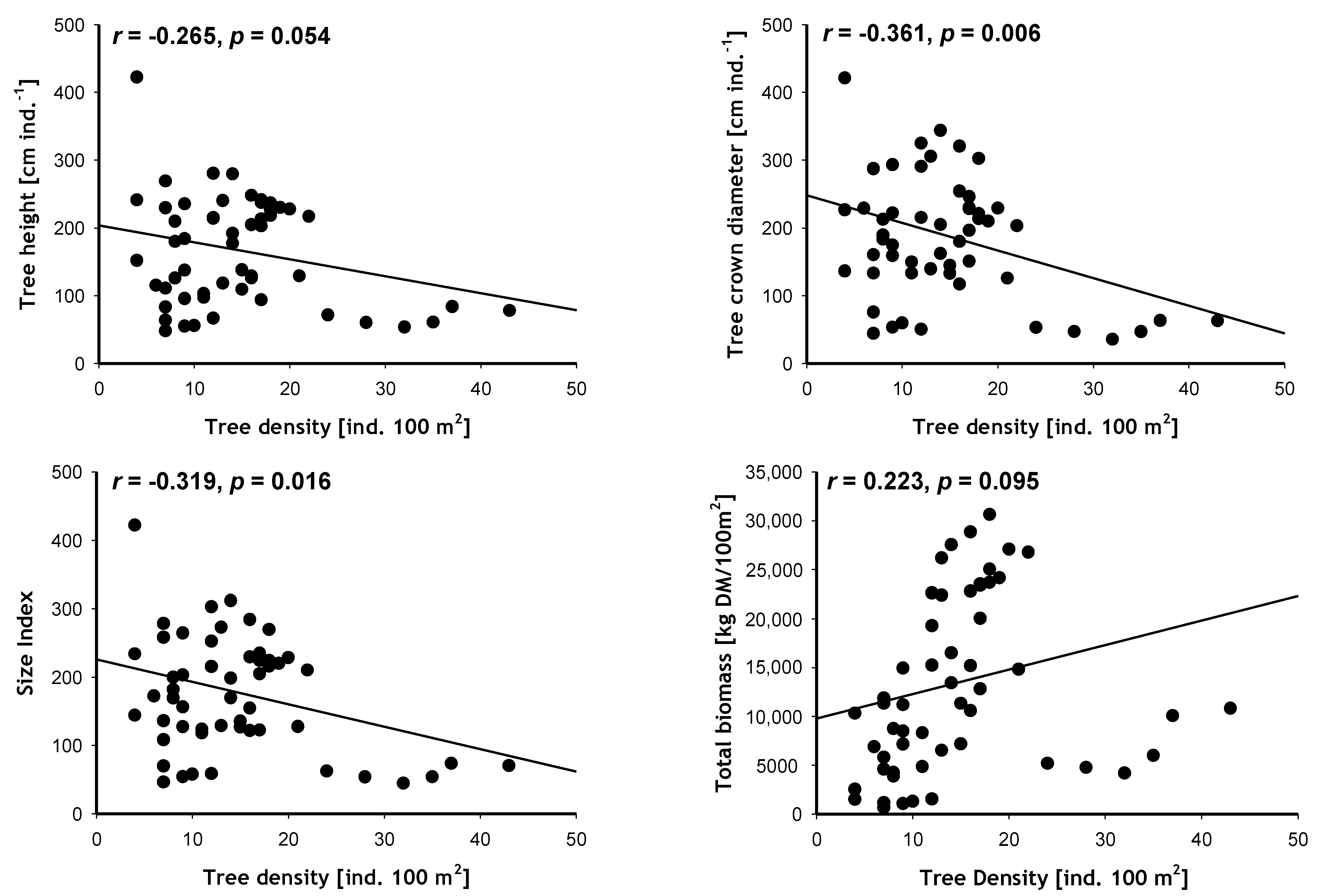
Results also indicated a negative correlation between tree size characteristics and mangrove density, i.e., the larger the size index, height, or crown diameter of each tree, the less dense the forest is likely to be (Figure 5).

Interestingly, it is the density factor and not the individual size factor that is positively correlated with total biomass; counter-intuitively, it is the shorter but denser central mangroves that possess a higher total biomass, rather than the taller but sparser northern ones.

4. Discussion

In accordance with existing research [14,65,66], these results illustrated the critical dependence of natural carbon stocks and plant establishment in A. marina forests on multiple environmental factors. They also served to demonstrate how, even when within the same or very similar habitats, these factors can change dramatically, causing observable alterations to the ecosystems. It can be inferred from the results that the increase in TN and TP had a negative effect on the tree density characteristic of the mangroves, and that greater values for EC and TDS contributed positively to tree height. Both the sediment analyses and the water analyses indicated the mangroves in the central location held the greatest magnitude for TP and TN values, whereas the northern location was shown to have held the smallest. Despite similar findings from both sediment and sea water analyses in those areas, the sediment analyses suggest that the central location possesses the highest EC and TDS values, whereas the water analyses evince a decreasing gradient for those values progressing from north to south.

In terms of the productivity of the mangroves, both the nutrient abundance and salinity have been shown to have an influence. Given the elevated salinity levels in both the northern and central locations, it has been suggested that A. marina growing there would experience physiological stress, as they would have to focus a greater proportion of their energy on osmotic regulation, as opposed to growth [10,67,68]. Arshad et al. [59] asserted this link as causative in their research, stating the salinity levels have direct and negative implications for stem and leaf development. In addition to the salinity level impact at the central site, a higher degree of pollution was observed there, likely from a combination of fertiliser run-off, residential wastewater, industrial point sources, and other human activities [21,69], contributing to the ongoing eutrophication of the water. Aside from causing eutrophication, a further contributor of physiological stress, the pollution itself also negatively affects the survivability of mangroves, as Vaiphasa et al. [70] found in their observation, wherein effluents from shrimp ponds were in the vicinity. Arshad et al. [59] further argued that the improper disposal of sewage into the water was causing mangrove pneumatophores to die off. This directly impedes plant growth, as the respiration rate of the root system cannot keep up with nutrient uptake with its pollution-reduced aeration surface area [71]. In all, existing studies by Saifullah [49], Alongi [72], and Triantafyllou et al. [73], seem to align with the results from this research, suggesting reliability.

The results align with previous research, suggesting that the relatively small size and fragmentary distribution of mangroves in the central location has many contributing factors, including alterations in land use, low level of precipitation, a stiffer substrate, significantly high concentrations of nitrogen and phosphorous in sea water and substrates, and pollution types and levels [21,32,49,72,74]. However, it still cannot be stated with certainty from the new results in this paper whether or not intraspecific competition may be an additional reason. Shaltout and Ayyad [75] proposed that, given the growth of a plant more tightly encompassed by others is less in comparison with a plant that has more space [76], the indirect correlation in the central location between small size and high density could be partly explained by intraspecific competition. In comparison to the central location, the data from the southern location could be argued to indicate intraspecific competition is a factor, as its high tree size but relatively low density suggests the size was augmented by a decrease in that competition. Nonetheless, this study presents data that also seems to indicate that the density change from southern to central locations is triggered by the differing levels of TN and TP in the sea water and sediments, not intraspecific competition. For this to be known for certain, more empirical studies would be necessary to specifically investigate how intraspecific competition affects population characteristics and dynamics of Saudi Red Sea coast mangroves. Existing research has also presented similar overall results [18,58,75,77,78,79,80]. Appearing to signify a negative correlation between tree density and tree size factors (height and crown diameter), and a positive correlation between overall biomass and tree density, the results from this research continue to be in accordance with earlier studies (e.g., Fromard et al. [81]; Xiao [82]; Slik [83]; Eid et al. [84]; Fajardo [85]) and predicted outcomes. As previously stated, the results infer that the total biomass per unit area of each location varies as a result of the size and density of the trees.

At 1188.2 Mg DM ha⁻¹ in the south, total biomass was found to incrementally decline northwards, to 660.9 Mg DM ha⁻¹ in the centre, and down to 197.9 Mg DM ha⁻¹ in the north. It is highly probable that this gradient is caused by the southernmost zone’s relatively high precipitation, nutrient abundance, higher quantity of wadis, tropical climate, and slightly reduced salinity [32,49], as was observed in the measured environmental properties. The average AGB for this dataset was 469.4 Mg DM ha⁻¹ (

Table 8. Mean of above ground biomass [AGB: Mg DM ha⁻¹], below ground biomass [BGB: Mg DM ha⁻¹] and total carbon [TC: Mg C ha⁻¹] of Avicennia marina populations along the Red Sea coast of Saudi Arabia compared with those reported in different mangrove forests around the globe.

Location	AGB	BGB	TC	Reference
Red Sea coast, Saudi Arabia	469.4	212.9	264.9	Present study
Gebel Elba Protected Area, Egypt			33.8	Afefe et al. [91]
South Sinai, Egypt	201.0	32.9	109.3	Omar [88]
Mangrove global average	115.2			Hu et al. [86]
Mangrove global average		78.6		Hutchison et al. [95]
Zambezi River Delta, Mozambique	192–252			Fatoyinbo et al. [96]
Sofala Bay, Mozambique	134.6		58.6	Sitoe et al. [87]
Arabian Gulf, United Arab Emirates	77.6	63.2	7.3–147.5	Schile et al. [10]
Kerala, India	80.2	36.9	58.6	Harishma et al. [97]
Central Kalimantan, Indonesia	68.8	28.4	45.7	Junaedi et al. [98]
West Papua Province, Indonesia			113.0	Sasmito et al. [24]
Sulawesi, Indonesia	12.1–182.2	2.7–70.8		Cameron et al. [99]
East Sumatra, Indonesia	40.7–279.0			Kusmana et al. [100]
Coastal wetlands, Indonesia			175.8	Alongi et al. [101]
Andaman Coast, Thailand	250.0	95.0	155.0	Jachowski et al. [102]
Southern Thailand	159.0			Christensen [103]
Okukubi River, Japan	162.7	125.1		Kamruzzaman et al. [104]
Ishigaki Island, Japan	94.8			Suzuki and Tagawa [105]
Northeast Hainan Island, China	119.3			Wang et al. [41]
Queensland, Australia	204.3	118.7		Mackey [45]
Ajuruteua Peninsula, Brazil	88.3	83.8	72.9	Virgulino-Júnior et al. [66]
Laguna de Terminos, Mexico		9.9		Perez-Ceballos et al. [106]
Dominican Republic	123.5–383.5	2.7–13.8		Sherman et al. [107]

Mg: 10³ kg.

), which was significantly higher than the global mangrove AGB average Hu et al. [86] proposed of 115.2 Mg DM ha⁻¹, and also higher than the averages of mangroves in many countries (e.g., United Arab Emirates, Australia, Japan, and Egypt). Sitoe et al. [87] asserted that the average tree height causes this significant variance in the biomasses of the same species; however, Abohassan et al. [46] purport that it is the environmental conditions instead that have greater influence. Each location’s relative proportions of AGB to BGB of the total biomass also diverged conspicuously; the southern location’s AGB was 74.3% of its total, the central location’s AGB was 62.1% of its total, and the northern location’s AGB was 58.4%. These values are akin to results found for the same or similar mangroves within analogous environments; measurements of the Sinai Peninsula’s salt plain (78% AGB) and southern coastline (75.3% AGB) are accordant with the southern location’s AGB [88]. For the northern or central locations, it is the transplanted mangroves in Egypt’s Nabq and Ras Mohammed Protected Area (53.1% AGB) [88], Bangladesh’s Oligohaline zone of the Sundarbans (64.8% AGB) [89], and Mozambique’s Sofala Bay (52% AGB) [87] that show similar values. Biomass overall was purported to differ considerably over climate gradients by Simard et al. [90], and a significant number of authors concur that geomorphological settings also have a substantial impact on biomass [25,26,66]. Although the proportion of AGB was still greater than BGB in the central and northern locations, they were both significantly closer to being evenly split than the southern zone; i.e., the BGB-to-AGB ratios were 0.7 in the north, 0.6 in the centre, and 0.4 in the south. It is possible that A. marina, prioritising establishment of a supportive and stable root network at early stages to compensate for oxygen-deprived loose sediments, grows more AGB as it matures and augments its biomass [27]. The southern location, possessing the greatest overall biomass, also possessed the largest biomass carbon content, at 412.5 Mg C ha⁻¹. Values of 294.6 Mg C ha⁻¹ and 87.6 Mg C ha⁻¹ were calculated for the central and northern locations, respectively. Results shared by Mashaly et al. [27] investigating A. marina show a value of 109.3 Mg C ha⁻¹ in southern Sinai for intertidal mangrove forests. As can be seen in Table 8, the average total biomass carbon content was 264.9 Mg C ha⁻¹ for this study, comparative averages from other studies suggest this is fairly high: Schile et al. [10] reported 7.3–147.5 Mg C ha⁻¹ from the UAE, Afefe et al. [91] had 33.8 Mg C ha⁻¹ for Egypt’s Gebel Elba Protected Area, and Sitoe et al. [87] found an average in Mozambique’s Sofala Bay of 264.9 Mg C ha⁻¹. Furthermore, a higher AGB carbon value than average was also determined in this study (180.3 Mg C ha⁻¹), when compared with the mean AGB carbon values of 40.2 and 125 Mg C ha⁻¹ for Australian [92] and New Zealand [93] mangroves, respectively. Contrastingly, and despite a higher than average value for AGB carbon, the BGB carbon values calculated for the three locations averaged at 84.6 Mg C ha⁻¹, much lower than the largest reported value worldwide (263 Mg C ha⁻¹), and still significantly lower than an average obtained for a study in Brazil (104.4 Mg C ha⁻¹) by Santos et al. [94]. These discrepancies could be explained by the hydrogeomorphic setting directing the mangrove’s blue carbon stock dynamics, in parallel to long-term transformations of land-use having a significant impact on carbon gains and losses [24].

Despite having such a crucial role in counteracting climate change and sequestering carbon [14,108,109], mangrove forests are one of the worst-suffering ecosystems, deteriorating at an alarming rate [108,110,111,112,113]. According to Almahasheer et al. [31], a 12% augmentation of the area of mangroves has been provoked by governmental initiatives along the Red Sea coastline in the past 40 years. Even with this level of input, the degree of risk to mangroves in the area continues to climb, with existing factors’ effects being exacerbated by new ones, such as excessive tree felling and grazing, the development of resorts or the oil industry [114], invasion of territory by shrimp farmers [53], and pollution from sewage and oil [80]. In 2017, to tackle this issue and be held accountable and responsible for protecting the mangrove habitats, the Council of Ministers of Saudi Arabia created the Standing Committee for the Protection of the Environment of Coastal Areas. While this committee is a landmark first step in the road to preserving Red Sea coast mangroves, more work will be necessary to reap their other benefits, and improve upon not only the mangroves’ quality, but also their capacity to sequester carbon.

5. Conclusions

By devising equations for rapid, cost-effective, and sustainable biomass estimation of A. marina mangroves along the Saudi Red Sea coast, this innovative and unobtrusive method is now readily applicable by relevant authorities responsible for conservation—not only along the Saudi part of the Red Sea coast, but also in various other locations encircling Red Sea. The mangrove (A. marina) of the Saudi Arabia Red Sea coast showed a gradual increase in the overall tree biomass and total biomass carbon storage from the north to the south. These results serve to accurately illustrate the way by which biomass production and carbon storage of A. marina mangrove forests along a significant portion of the Red Sea coast are influenced by nutrient availability and salinity. These equations and results are important, as in order to preserve the environment and attenuate the emissions of carbon dioxide into the atmosphere, finding a way to revitalise and restore mangroves and other marine ecosystems will be crucial.

References

1. IPCC. Understanding and Attributing Climate Change; Cambridge University Press: Cambridge, UK; New York, NY, USA, 2007; Volume 9, pp. 665–717. [Google Scholar]
2. Australian Academy of Science. The Science of Climate Change, Questions and Answers. 2015. Available online: https://www.interacademies.org/sites/default/files/publication/climatechange2010_1.pdf (accessed on 15 April 2021).
3. Page, M.L. Carbon dioxide levels will soar past the 410 ppm milestone in 2019. New Sci. 2019, 3214, 1–3. [Google Scholar]
4. Pendleton, L.; Donato, D.C.; Murray, B.C.; Crooks, S.; Jenkins, W.A.; Sifleet, S.; Craft, C.; Fourqueran, J.W.; Kauffman, J.B.; Marbà, N.; et al. Estimating Global “Blue Carbon” Emissions from Conversion and Degradation of Vegetated Coastal Ecosystems. PLoS ONE 2012, 7, e43542. [Google Scholar]
5. Keesstra, S.; Sannigrahi, S.; López-Vicente, M.; Pulido, M.; Novara, A.; Visser, S.; Kalantari, Z. The role of soils in regulation and provision of blue and green water. Philos. Trans. R. Soc. B 2021, 376, 20200175. [Google Scholar] [CrossRef]
6. Keesstra, S.; Mol, G.; De Leeuw, J.; Okx, J.; Molenaar, C.; De Cleen, M.; Visser, S. Soil-Related Sustainable Development Goals: Four Concepts to Make Land Degradation Neutrality and Restoration Work. Land 2018, 7, 133. [Google Scholar] [CrossRef] [Green Version]
7. Jenny, H. The Soil Resource: Origin and Behavior; Springer: New York, NY, USA, 1980; 377p. [Google Scholar]
8. Lal, R. Soil carbon sequestration to mitigate climate change. Geoderma 2004, 123, 1–22. [Google Scholar] [CrossRef]
9. Hossain, M.D.; Nuruddin, A.A. Soil and Mangrove: A Review. J. Environ. Sci. Technol. 2016, 9, 198–207. [Google Scholar] [CrossRef] [Green Version]
10. Schile, L.; Kauffman, J.; Crooks, S.; Fourqurean, J.; Glavan, J.; Megonigal, J. Limits on carbon sequestration in arid blue carbon ecosystems. Ecol. Appl. 2017, 27, 859–874. [Google Scholar] [CrossRef] [PubMed]
11. Chowdhury, A.; Naz, A.; Bhattacharyya, S.; Sanyal, P. Cost–benefit analysis of ‘Blue Carbon’ sequestration by plantation of few key mangrove species at Sundarban Biosphere Reserve, India. Carbon Manag. 2019, 9, 575–586. [Google Scholar] [CrossRef]
12. Jones, A.R.; Segaran, R.; Clarke, K.D.; Waycott, M.; Goh, W.S.H.; Gillanders, B.M. Estimating Mangrove Tree Biomass and Carbon Content: A Comparison of Forest Inventory Techniques and Drone Imagery. Front. Mar. Sci. 2020, 6, 784. [Google Scholar] [CrossRef] [Green Version]
13. Taillardat, P.; Friess, D.A.; Lupascu, M. Mangrove blue carbon strategies for climate change mitigation are most effective at the national scale. Biol. Lett. 2018, 14, 20180251. [Google Scholar] [CrossRef] [PubMed]
14. Ouyang, X.; Lee, S.Y. Improved estimates on global carbon stock and carbon pools in tidal wetlands. Nat. Commun. 2020, 11, 317. [Google Scholar] [CrossRef] [PubMed] [Green Version]
15. Twilley, R.R.; Chen, R.H.; Hargis, T. Carbon sinks in mangrove forests and their implications to the carbon budget of tropical coastal ecosystems. Water Air Soil Pollut. 1992, 64, 265–288. [Google Scholar] [CrossRef]
16. PERSGA/GEF. Status of Mangroves in the Red Sea and Gulf of Aden; PERSGA Technical Series No. 11; PERSGA (Regional Organization for the Conservation of the Environment of the Red Sea and Gulf of Aden): Jeddah, Saudi Arabia, 2004. [Google Scholar]
17. Almahasheer, H. Ecosystem Services of Avicennia marina in the Red Sea. Ph.D. Thesis, King Abdullah University of Science and Technology, Thuwal, Saudi Arabia, 2016. [Google Scholar]
18. Eid, E.M.; El-Bebany, A.F.; Alrumman, S.A. Distribution of soil organic carbon in the mangrove forests along the southern Saudi Arabian Red Sea coast. Rend. Fis. Acc. Lincei 2016, 27, 629–637. [Google Scholar] [CrossRef]
19. Shaltout, K.H. Economic and Environmental Values of Mangroves in Arabic Region. In Proceedings of the First Saudi Conference on Environment: Sustainable Management of Natural Resources, Abha, Saudi Arabia, 7–9 March 2016. [Google Scholar]
20. Robertson, A.I.; Phillips, M.J. Mangroves as filters of shrimp pond effluent: Prediction and biogeochemical research needs. Hydrobiologia 1995, 295, 311–321. [Google Scholar] [CrossRef]
21. Almahasheer, H.; Serrano, O.; Duarte, C.; Arias-Ortiz, A.; Masque, P.; Irigoien, X. Low carbon sink capacity of Red Sea mangroves. Sci. Rep. 2017, 7, 10. [Google Scholar] [CrossRef] [PubMed] [Green Version]
22. Bunting, P.; Rosenqvist, A.; Lucas, R.M.; Rebelo, L.M.; Hilarides, L.; Thomas, N.; Hardy, A.; Itoh, T.; Shimada, M.; Finlayson, C.M. The global mangrove watch—A new 2010 global baseline of mangrove extent. Remote Sens. 2018, 10, 1669. [Google Scholar] [CrossRef] [Green Version]
23. Jennerjahn, T.C.; Ittekkot, V. Relevance of mangroves for the production and deposition of organic matter along tropical continental margins. Naturwissenschaften 2002, 89, 23–30. [Google Scholar] [CrossRef]
24. Sasmito, S.D.; Sillanpää, M.; Hayes, M.A.; Bachri, S.; Saragi-Sasmito, M.F.; Sidik, F.; Hanggara, B.B.; Mofu, W.Y.; Rumbiak, V.I.; Taberima, S.; et al. Mangrove blue carbon stocks and dynamics are controlled by hydrogeomorphic settings and land-use change. Glob Chang. Biol. 2020, 26, 3028–3039. [Google Scholar] [CrossRef] [PubMed] [Green Version]
25. Rovai, A.S.; Twilley, R.R.; Castañeda-Moya, E.; Riul, P.; Miguel, C.; Manrow, M.; Horta, P.A.; Simonassi, J.C.; Fonseca, A.D.O.; Pagliosa, P.R. Global controls on carbon storage in mangrove soils. Nat. Clim. Chang. 2018, 8, 534–538. [Google Scholar] [CrossRef]
26. Twilley, R.R.; Rovai, A.S.; Riul, P. Coastal morphology explains global blue carbon distributions. Front. Ecol. Environ. 2018, 16, 503–508. [Google Scholar] [CrossRef] [Green Version]
27. Mashaly, I.; Hegazy, A.; Abdelaal, M.; El-Hussieny, S. Habitat-Based Estimate of Carbon Content in Mangrove Avicennia marina (Forssk.) Vierh. of South Sinai, Egypt. IOSR J. Environ. Sci. Toxicol. Food Technol. 2016, 10, 8–14. [Google Scholar]
28. Valiela, I.; Bowen, J.L.; York, J.K. Mangrove forests: One of the world’s threatened major tropical environments. Bioscience 2001, 51, 807–815. [Google Scholar] [CrossRef] [Green Version]
29. Alongi, D.M. Present state and future of the world’s mangrove forests. Environ. Conserv. 2002, 29, 331–349. [Google Scholar] [CrossRef] [Green Version]
30. Edwards, F.J.; Head, S.M. Key Environment: Red Sea; Pergamon Press: Oxford, UK, 1987; p. 451. [Google Scholar]
31. Almahasheer, H.; Aljowair, A.; Duarte, C.M.; Irigoien, X. Decadal stability of Red Sea mangroves. Estuar. Coast. Shelf Sci. 2016, 169, 164–172. [Google Scholar] [CrossRef] [Green Version]
32. Kumar, A.; Asif Khan, M.; Muqtadir, A. Distribution of Mangroves along the Red Sea Coast of the Arabian Peninsula: Part-1: The Northern Coast of Western Saudi Arabia. Earth Sci. India 2010, 3, 28–42. [Google Scholar]
33. Saifullah, S.M. Mangrove ecosystem of Saudi Arabian Red Sea coast-an overview. J. KAU Mar. Sci. 1994, 7, 263–270. [Google Scholar] [CrossRef]
34. Price, A.; Jobbins, G.; Dawson Shepherd, A.; Ormond, R. An integrated environmental assessment of the Red Sea coast of Saudi Arabia. Environ. Conserv. 1998, 25, 65–76. [Google Scholar] [CrossRef]
35. Woomer, P.L.; Tieszen, L.L.; Tappan, G.; Touré, A.; Sall, M. Land use change and terrestrial carbon stocks in Senegal. J. Arid Environ. 2004, 59, 625–642. [Google Scholar] [CrossRef]
36. Eid, E.M.; Shaltout, K.H. Distribution of soil organic carbon in the mangrove Avicennia marina (Forssk.) Vierh. along the Egyptian Red Sea coast. Reg. Stud. Mar. Sci. 2016, 3, 76–82. [Google Scholar] [CrossRef]
37. Jacotot, A.; Gensous, S.; Marchand, C.; Allenbach, M. Effects of elevated atmospheric CO2 and increased tidal flooding on leaf gas-exchange parameters of two common mangrove species: Avicennia marina and Rhizophora stylosa. Photosynth. Res. 2018, 138, 249–260. [Google Scholar] [CrossRef]
38. Ajonina, G.M. Inventory and Modelling Mangrove Forest Stand Dynamics Following Different Levels of Wood Exploitation Pressures in the Douala-Edea Atlantic Coast of Cameroon, Central Africa. Ph.D. Thesis, Albert-Ludwigs-Universität, Freiburg im Breisgau, Germany, 2008. [Google Scholar]
39. Kairo, J.G.; Lang’at, J.K.S.; Dahdouh-Guebas, F.; Hansen, L.; Bosire, J.O.; Karachi, M. Structural development and productivity of replanted mangrove plantations in Kenya. Forest Ecol. Manag. 2008, 255, 2670–2677. [Google Scholar] [CrossRef]
40. Alongi, D.M. The Energetics of Mangrove Forests, 1st ed.; Springer: Dordrecht, The Netherlands, 2010. [Google Scholar]
41. Wang, D.; Wan, B.; Liu, J.; Su, Y.; Guo, Q.; Qiu, P.; Wu, X. Estimating aboveground biomass of the mangrove forests on northeast Hainan Island in China using an upscaling method from field plots, UAV-LiDAR data and Sentinel-2 imagery. Int. J. Appl. Earth Obs. Geoinf. 2020, 85, 101986. [Google Scholar] [CrossRef]
42. Parvaresh, H.; Parvaresh, E.; Zahedi, G. Establishing allometric relationship using crown diameter for the estimation of above-ground biomass of grey mangrove, Avicennia marina (Forsk) Vierh in mangrove forests of Sirik, Iran. J. Basic Appl. Sci. Res. 2012, 2, 1763–1769. [Google Scholar]
43. Tran, P.; Leuzinger, S.; Alfaro, A.C. Allometry, Biomass and Litter Decomposition of the New Zealand Mangrove Avicennia marina var. australasica. Ph.D. Thesis, School of Applied Sciences, Auckland University of Technology, Auckland, New Zealand, 2014. [Google Scholar]
44. Tamooh, F.; Huxhamd, M.; Karachi, M.; Mencuccini, M.; Kairo, J.G.; Kirui, B. Below-ground root yield and distribution in natural and replanted mangrove forests at Gazi bay, Kenya. For. Ecol. Manag. 2008, 256, 1290–1297. [Google Scholar] [CrossRef]
45. Mackey, A.P. Biomass of the Mangrove Avivennia marina (Forssk.) Vierh. Near Brisbane, South-Eastern Queensland. Aust. J. Mar. Freshw. Res. 1993, 44, 721–725. [Google Scholar] [CrossRef]
46. Abohassan, R.A.; Okia, C.A.; Agea, J.G.; Kimondo, J.M.; McDonald, M.M. Perennial biomass production in arid mangrove systems on the Red Sea coast of Saudi Arabia. Environ. Res. J. 2012, 6, 22–31. [Google Scholar]
47. Novara, A.; Pulido, M.; Rodrigo-Comino, J.; Di Prima, S.; Smith, P.; Gristina, L.; Giminez-Morera, A.; Terol, E.; Salesa, D.; Keesstra, S. Long-term organic farming on a citrus plantation results in soil organic carbon recovery. Cuadernos de Investigación Geográfica 2019, 45, 271–286. [Google Scholar] [CrossRef] [Green Version]
48. Bruckner, A. Habitat Mapping and Characterization of Coral Reefs of the Saudi Arabian Red Sea: 2006–2009; Final Report Part II; Qisbah, R., Al Wajh, Y., Banks, F., Islands, F., Eds.; Khaled Bin Sultan Living Oceans Foundation, Panoramic Press: Phoenix, AZ, USA, 2011; 140p. [Google Scholar]
49. Saifullah, S.M. Mangrove ecosystem of Red Sea coast (Saudi Arabian). Pak. J. Mar. Sci. 1997, 6, 115–124. [Google Scholar] [CrossRef]
50. Siraj, A. Climate of Saudi Arabia. Climatic Features of Saudi Arabia. In Fauna of Saudi Arabia; Buttiker, W., Krupp, F., Eds.; National Commission for Wildlife Conservation and Development: Riyadh, Saudi Arabia, 1984; Volume 6, pp. 32–42. [Google Scholar]
51. Morley, N.J.F. The coastal waters of the Red Sea. Bull. Mar. Res. Cen. 1975, 5, 8–19. [Google Scholar]
52. El-Juhany, L.I. Present status and degradation trends of mangrove forests on the southern Red Sea coast of Saudi Arabia. Am. Euras. J. Agric. Environ. Sci. 2009, 6, 328–340. [Google Scholar]
53. Eid, E.M.; Arshad, M.; Shaltout, K.H.; El-Sheikhe, M.A.; Alfarhan, A.H.; Picó, Y.; Barcelo, D. Effect of the conversion of mangroves into shrimp farms on carbon stock in the sediment along the southern Red Sea coast, Saudi Arabia. Environ. Res. 2019, 176, 108536. [Google Scholar] [CrossRef]
54. Shaltout, K.H.; Ahmed, M.T.; Alrumman, S.A.; Ahmed, D.A.; Eid, E.M. Evaluation of the carbon sequestration capacity of arid mangroves along nutrient availability and salinity gradients along the Red Sea coastline of Saudi Arabia. Oceanologia 2019, 62, 56–69. [Google Scholar] [CrossRef]
55. Mandura, A.S.; Khafaji, A.K.; Saifullah, S.M. Ecology of a mangrove stand of a central Red Sea coast area: Ras Hatiba (Saudi Arabia). Proc. Saudi Biol. Soc. 1988, 11, 85–112. [Google Scholar]
56. El-Demerdash, M.A. Vegetation of the Farasan Islands, Red Sea, Saudi Arabia. J. Veg. Sci. 2009, 7, 81–88. [Google Scholar] [CrossRef]
57. Almahasheer, H.; Duarte, C.; Irigoien, X. Phenology and growth dynamics of Avicennia marina in the central Red Sea. Sci. Rep. 2016, 6, 37785. [Google Scholar] [CrossRef] [PubMed] [Green Version]
58. Almahasheer, H.; Duarte, C.; Irigoien, X. Nutrient limitation in central Red Sea mangroves. Front. Mar. Sci. 2016, 3, 271. [Google Scholar] [CrossRef] [Green Version]
59. Arshad, M.; Alrumman, S.; Eid, E.M. Evaluation of carbon sequestration in the sediment of polluted and non-polluted locations of mangroves. Fund. Appl. Limnol. 2018, 192, 53–64. [Google Scholar] [CrossRef]
60. Strickland, J.D.; Parsons, T.R. Determination of reactive phosphorus. In A Practical Handbook of Seawater Analysis; Fisheries Research Board of Canada: Ottawa, ON, Canada, 1972; Volume 167, pp. 49–56. [Google Scholar]
61. Novozamsky, I.; van Eck, R.; van Schouwenburg, J.; Walinga, I. Total nitrogen determination in plant material by means of the indophenol blue method. Neth. J. Agric. Sci. 1974, 22, 3–13. [Google Scholar]
62. Kauffman, J.B.; Donato, D.C. Protocols for the Measurement, Monitoring, and Reporting of Structure, Biomass and Carbon Stocks in Mangrove Forests; Center for International Forest Research: Bogor, Indonesia, 2012. [Google Scholar]
63. SPSS. SPSS Base 15.0 User’s Guide; SPSS Inc.: Chicago, IL, USA, 2006. [Google Scholar]
64. Ter Braak, C.J.F.; Smilauer, P. Canoco Reference Manual and User’s Guide: Software for Ordination (Version 5.0); Microcomputer Power: Ithaca, NY, USA, 2012. [Google Scholar]
65. Quinn, L.D.; Rauterkus, M.A.; Holt, J.S. Effects of nitrogen enrichment and competition on growth and spread of giant reed (Arundo donax). Weed Sci. 2007, 55, 319–326. [Google Scholar] [CrossRef]
66. Virgulino-Júnior, P.; Carneiro, D.N.; Nascimento, W.R., Jr.; Cougo, M.F.; Fernandes, M. Biomass and carbon estimation for scrub mangrove forests and examination of their allometric associated uncertainties. PLoS ONE 2020, 15, e0230008. [Google Scholar] [CrossRef] [PubMed]
67. Alongi, D.M. Carbon cycling and storage in mangrove forests. Annu. Rev. Mar. Sci. 2014, 6, 195–219. [Google Scholar] [CrossRef] [PubMed]
68. Rahman, M.M.; Islam Khan, N.M.; Hoque, F.A.K.; Ahmed, I. Carbon stock in the Sundarbans mangrove forest: Spatial variations in vegetation types and salinity zones. Wetl. Ecol. Manag. 2015, 23, 269–283. [Google Scholar] [CrossRef]
69. Touliabah, H.E.; Abu El-Kheir, W.S.; Kuchari, M.G.; Abdulwassi, N.I.H. Phytoplankton composition at Jeddah Coast–Red Sea, Saudi Arabia in relation to some ecological factors. JKAU Sci. 2010, 22, 115–131. [Google Scholar] [CrossRef] [Green Version]
70. Vaiphasa, C.; de Boer, W.F.; Skidmore, A.K.; Panitchart, S.; Vaiphasa, T.; Bamrongrugsa, N.; Santitamnont, P. Impact of solid shrimp pond waste materials on mangrove growth and mortality: A case study from Pak Phanang, Thailand. Hydrobiologia 2007, 591, 47–57. [Google Scholar] [CrossRef]
71. Mandura, A.S. A mangrove stand under sewage pollution stress: Red Sea. Mangroves Salt Marshes 1997, 1, 255–262. [Google Scholar] [CrossRef]
72. Alongi, D.M. Early growth responses of mangroves to different rates of nitrogen and phosphorus supply. J. Exp. Mar. Biol. Ecol. 2011, 397, 85–93. [Google Scholar] [CrossRef]
73. Triantafyllou, G.; Yao, F.; Petihakis, G.; Tsiaras, K.; Raitsos, D.; Hoteit, I. Exploring the Red Sea seasonal ecosystem functioning using a three-dimensional biophysical model. J. Geophys. Res. Ocean. 2014, 119, 1791–1811. [Google Scholar] [CrossRef] [Green Version]
74. Naidoo, G. Differential effects of nitrogen and phosphorus enrichment on growth of dwarf Avicennia marina mangroves. Aquat. Bot. 2009, 90, 184–190. [Google Scholar] [CrossRef]
75. Shaltout, K.H.; Ayyad, M. Structure and standing crop of Egyptian Thymelaea hirsuta populations. Vegetatio 1988, 74, 137–142. [Google Scholar] [CrossRef]
76. Weiner, J. Neighbourhood interference amongst Pinus rigida individuals. J. Ecol. 1984, 72, 183–195. [Google Scholar] [CrossRef]
77. Shaltout, K.H.; Ayyad, M. Phytosociological Behavior of Thymelaea hirsuta (L.) Endl. in Egypt. Flora 1994, 189, 193–199. [Google Scholar] [CrossRef]
78. Sato, G.; Negassi, S.; Tahiri, A. The only elements required by plants that are deficient in sea water are nitrogen, phosphorous and iron. Cytotechnology 2011, 63, 201–204. [Google Scholar] [CrossRef] [PubMed] [Green Version]
79. Afefe, A.A. Ecology and Distribution of Mangrove Forest in Egypt. In The 3rd Near-East Forestry Week and 21st Session of the Near East Forestry and Range Commission Side Event Theme: Green Economy; FAO Office: Amman, Jordan, 2014. [Google Scholar]
80. Shaltout, K.H.; El-Bana, M.I.; Eid, E.M. Ecology of the Mangrove Forests along the Egyptian Red Sea Coast; LAP Lambert Academic Publishing: Saarbrücken, Germany, 2018. [Google Scholar]
81. Fromard, F.; Puig, H.; Mougin, E.; Marty, G.; Betoulle, J.L.; Cadamuro, L. Structure, above-ground biomass and dynamics of mangrove ecosystems: New data from French Guiana. Oecologia 1998, 115, 39–53. [Google Scholar] [CrossRef]
82. Xiao, S.; Chen, S.; Zhao, L.; Gang, W. Density Effects on Plant Height Growth and Inequality in Sunflower Populations. J. Integr. Plant Biol. 2006, 48, 513–519. [Google Scholar] [CrossRef]
83. Slik, J.F.; Paoli, G.; McGuire, K.; Amaral, I.; Barroso, J.; Bastian, M.; Blanc, L.; Bongers, F.; Boundja, P.; Clark, C.; et al. Large trees drive forest aboveground biomass variation in moist lowland forests across the tropics. Glob. Ecol. Biogeogr. 2013, 22, 1261–1271. [Google Scholar] [CrossRef]
84. Eid, E.M.; Youssef, M.S.G.; Shaltout, K.H. Population characteristics of giant reed (Arundo donax L.) in cultivated and naturalized habitats. Aquat. Bot. 2016, 129, 1–8. [Google Scholar] [CrossRef]
85. Fajardo, A. Insights into intraspecific wood density variation and its relationship to growth, height and elevation in a tree line species. Plant Biol. 2018, 20, 456–464. [Google Scholar] [CrossRef]
86. Hu, T.; Zhang, Y.; Su, Y.; Zheng, Y.; Lin, G.; Guo, Q. Mapping the Global Mangrove Forest Aboveground Biomass Using Multisource Remote Sensing Data. Remote Sens. 2020, 12, 1690. [Google Scholar] [CrossRef]
87. Sitoe, A.A.; Mandlate, L.J.C.; Guedes, B.S. Biomass and carbon stocks of Sofala Bay Mangrove Forests. Forests 2014, 5, 1967–1981. [Google Scholar] [CrossRef]
88. Omar, S. Evaluation of Atmospheric Carbon Dioxide Sequestration in Mangrove Ecosystem in South Sinai, Egypt. Ph.D. Thesis, Tanta University, Tanta, Egypt, 2017. [Google Scholar]
89. Kamruzzaman, M.; Ahmed, S.; Osawa, A. Biomass and net primary productivity of mangrove communities along the Oligohaline zone of Sundarbans, Bangladesh. For. Ecosyst. 2017, 4, 16. [Google Scholar] [CrossRef] [Green Version]
90. Simard, M.; Fatoyinbo, L.; Smetanka, C.; Rivera-Monroy, V.H.; Castañeda-Moya, E.; Thomas, N.; Van der Stocken, T. Mangrove canopy height globally related to precipitation, temperature and cyclone frequency. Nat. Geosci. 2019, 12, 40–45. [Google Scholar] [CrossRef]
91. Afefe, A.A.; Abbas, M.S.; Soliman, A.S.; Khedr, A.A.; Hatab, E.E. Tree biomass and soil carbon stocks of a mangrove ecosystem on the Egyptian-African Red Sea coast. Fundam. Appl. Limnol. 2020, 193, 239–251. [Google Scholar] [CrossRef]
92. Serrano, O.; Lovelock, C.E.; Atwood, T.B.; Macreadie, P.I.; Canto, R.; Phinn, S.; Arias-Ortiz, A.; Bai, L.; Baldock, J.; Bedulli, C.; et al. Australian vegetated coastal ecosystems as global hotspots for climate change mitigation. Nat. Commun. 2019, 10, 4313. [Google Scholar] [CrossRef] [PubMed]
93. Suyadi; Gao, J.; Lundquist, C.J.; Schwendenmann, L. Aboveground Carbon Stocks in Rapidly Expanding Mangroves in New Zealand: Regional Assessment and Economic Valuation of Blue Carbon. Estuaries Coasts 2020, 43, 1456–1469. [Google Scholar] [CrossRef]
94. Santos, D.M.C.; Estrada, G.C.D.; Fernandez, V.; Estevam, M.R.M.; Souza, B.T.; Soares, M.L.G. First Assessment of Carbon Stock in the Belowground Biomass of Brazilian Mangroves. An. Acad. Bras. Ciênc. 2017, 89, 1579–1589. [Google Scholar] [CrossRef] [Green Version]
95. Hutchison, J.; Manica, A.; Swetnam, R.; Balmford, A.; Spalding, M. Predicting global patterns in mangrove forest biomass. Conserv. Lett. 2014, 7, 233–240. [Google Scholar] [CrossRef] [Green Version]
96. Fatoyinbo, T.; Feliciano, E.A.; Lagomasino, D.; Lee, S.K.; Trettin, C. Estimating mangrove aboveground biomass from airborne LiDAR data: A case study from the Zambezi River delta. Environ. Res. Lett. 2018, 13, 025012. [Google Scholar] [CrossRef] [Green Version]
97. Harishma, K.M.; Sandeep, S.; Sreekumar, V.B. Biomass and carbon stocks in mangrove ecosystems of Kerala, southwest coast of India. Ecol. Process. 2020, 9, 31. [Google Scholar] [CrossRef]
98. Junaedi, A.; Hidayat, N.; Mediawati, Y.; Wibowo, A.; Rizal, M.; Setiarno, I.; Surasana, N. Biomass, carbon stock and oxygen produced by mangrove vegetation in tropical forest in central Kalimantan, Indonesia. Asian J. Crop Sci. 2020, 12, 26–33. [Google Scholar] [CrossRef] [Green Version]
99. Cameron, C.; Hutley, L.B.; Friess, D.A.; Brown, B. Community structure dynamics and carbon stock change of rehabilitated mangrove forests in Sulawesi, Indonesia. Ecol. Appl. 2019, 29, e01810. [Google Scholar] [CrossRef] [Green Version]
100. Kusmana, C.; Sabiham, S.; ABE, K.; Watanabe, H. An estimation of above ground tree biomass of a mangrove forest in East Sumatra, Indonesia. Tropics 1992, 1, 243–257. [Google Scholar] [CrossRef] [Green Version]
101. Alongi, D.M.; Murdiyarso, D.; Fourqurean, J.W.; Kauffman, J.B.; Hutahaean, A.; Crooks, S.; Lovelock, C.E.; Howard, J.; Herr, D.; Fortes, M.; et al. Indonesia’s blue carbon: A globally significant and vulnerable sink for seagrass and mangrove carbon. Wetl. Ecol. Manag. 2016, 24, 3–13. [Google Scholar] [CrossRef]
102. Jachowski, N.; Quak, M.; Friess, D.; Duangnamon, D.; Webb, E.; Ziegler, A. Mangrove biomass estimation in Southwest Thailand using machine learning. Appl. Geogr. 2013, 45, 311–321. [Google Scholar] [CrossRef]
103. Christensen, B. Biomass and primary production of Rhizophora apiculata Bl. In a mangrove in southern Thailand. Aquat. Bot. 1978, 4, 43–52. [Google Scholar] [CrossRef]
104. Kamruzzaman, M.; Osawa, A.; Deshar, R.; Sharma, S.; Mouctar, K. Species composition, biomass, and net primary productivity of mangrove forest in Okukubi River, Okinawa Island, Japan. Reg. Stud. Mar. Sci. 2017, 12, 19–27. [Google Scholar] [CrossRef]
105. Suzuki, E.; Tagawa, H. Biomass of a mangrove forest and a sedge marsh on Ishigaki Island, South Japan. Jpn. J. Ecol. 1983, 33, 231–234. [Google Scholar]
106. Perez-Ceballos, R.; Rivera-Rosales, K.; Zaldivar-Jiménez, A.; Canales-Delgadillo, J.; Brito-Pérez, R.; Amador del Angel, L.; Merino-Ibarra, M. Effect of hydrological restoration on the productivity of underground roots in the mangroves of Laguna de Terminos, Mexico. Bot. Sci. 2018, 96, 569–581. [Google Scholar] [CrossRef]
107. Sherman, R.; Fahey, T.; Martinez, P. Spatial Patterns of Biomass and Aboveground Net Primary Productivity in a Mangrove Ecosystem in the Dominican Republic. Ecosystems 2003, 6, 384–398. [Google Scholar] [CrossRef]
108. Sanderman, J.; Hengl, T.; Fiske, G.; Solvik, K.; Adame, M.F.; Benson, L.; Bukoski, J.J.; Carnell, P.; Cifuentes-Jara, M.; Donato, D.; et al. A global map of mangrove forest soil carbon at 30 m spatial resolution. Environ. Res. Lett. 2018, 13, 055002. [Google Scholar] [CrossRef]
109. Al-Guwaiz, S.M.; Alatar, A.A.; El-Sheikh, M.A.; Al-Gehni, G.A.; Faisal, M.; Qahtan, A.A.; Abdel-Salam, E.M. Role of Mangrove Rehabilitation and Protection Plans on Carbon Storage in Yanbu Industrial City, Saudi Arabia: A Case Study. Sustainability 2021, 13, 13149. [Google Scholar] [CrossRef]
110. Siikamӓki, J.; Sanchirico, J.; Jardine, S. Global economic potential for reducing carbon dioxide emissions from mangrove loss. Proc. Natl. Acad. Sci. USA 2012, 109, 14369–14374. [Google Scholar] [CrossRef] [PubMed] [Green Version]
111. Chowdhury, A.; Naz, A.; Bhattacharyya, S. Plantation Methods and Restoration Techniques for Enhanced Blue Carbon Sequestration by Mangroves. In Sustainable Agriculture Reviews 37; Inamuddin, Asiri, A., Lichtfouse, E., Eds.; Springer: Cham, Switzerland, 2019; Volume 37. [Google Scholar]
112. Ouyang, X.; Lee, S.; Wang, W. The ‘Perfect’ Conversion: Dramatic Increase in CO2 Efflux from Shellfish Ponds and Mangrove Conversion in China. Sustainability 2021, 13, 13163. [Google Scholar] [CrossRef]
113. Quintero-Morales, M.A.; Plata-Rocha, W.; Monjardín-Armenta, S.A.; Olimón-Andalón, V.; Torres-Montoya, E.H. Geospatial Simulation Model of Sustainable Mangrove Development Scenarios for the Years 2030 and 2050 in Marismas Nacionales, Mexico. Sustainability 2021, 13, 9551. [Google Scholar] [CrossRef]
114. Hussain, M.; Khoja, T. Intertidal and subtidal blue-green algal mats of open and mangrove areas in the Farasan Archipelago (Saudi Arabia), Red Sea. Bot. Mar. 1993, 36, 377–388. [Google Scholar] [CrossRef]
Figure 1. Map of the study area indicating the sampling sites ( Sustainability 13 13996 i001).
Sustainability 13 13996 g001
Figure 2. Characteristics [mean ± standard error] of Avicennia marina populations along the Red Sea coast of Saudi Arabia. Vertical bars indicate the standard errors of the means. F-values represent the one-way ANOVA. Means followed by different letters are significantly different at p < 0.05 according to the Tukey’s HSD test.
Sustainability 13 13996 g002
Figure 3. CCA biplot with sediment characteristics [→] and population parameters [+] of Avicennia marina growing along the Red Sea coast of Saudi Arabia. EC: Electrical conductivity, TDS: Total dissolved solids, TP: Total phosphorus, TN: Total nitrogen.
Sustainability 13 13996 g003
Figure 4. CCA biplot with sea water characteristics [→] and population parameters [+] of Avicennia marina growing along the Red Sea coast of Saudi Arabia. EC: Electrical conductivity, TDS: Total dissolved solids, TP: Total phosphorus, TN: Total nitrogen.
Sustainability 13 13996 g004
Figure 5. The relation between some parameters of Avicennia marina populations along the Red Sea coast of Saudi Arabia. r-values represent Pearson correlation coefficient.
Sustainability 13 13996 g005