Influence of Different Allocation Methods for Recycling and Dynamic Inventory on CO₂ Savings and Payback Times of Light-Weighted Vehicles Computed under Product- and Fleet-Based Analyses: A Case of Internal Combustion Engine Vehicles

Abstract

Light weighting by material substitution is a key to reducing GHG emissions during vehicle operation. The GHG benefits are a salient factor in selecting lightweight materials for vehicles. Although the literature has performed lightweight material selections using GHG benefits under product- and fleet-based life-cycle inventory (LCI) analyses, recycling effects have therein been accounted for by arbitrarily selecting allocation methods for recycling, as the consensus on their selection is absent. Furthermore, studies have mistreated the temporal variations of the LCI parameters (the dynamic inventory (DI)), though that could be an important factor affecting the overall LCI results when allocation methods for recycling are in place. Therefore, to investigate their influence on greenhouse gas (GHG) benefit evaluations, an LCI case study was conducted, centered on aluminum- and magnesium-substituted internal combustion engine vehicles (ICEVs) at the product- and fleet- levels. “CO₂ savings” and the “CO₂ payback time”, as well as four allocation methods for recycling, were considered to represent the GHG benefits and address the recycling effects, respectively. The dynamic inventory was based on the world average electricity grid mix change. The results indicate that changing the conditions of the DI and the allocation methods for recycling could alter the better performing material under fleet-based analyses. Therefore, we ascertained that the choice of the allocation method for recycling and conducting fleet-scale dynamic LCI analyses in the presence of the DI is pivotal for material selections.

1. Introduction

The transportation sector is an important industrial sector in any economy that deals with the movement of people and products [1]. It includes air freight and logistics, airlines, and marine, road, rail, and transportation infrastructure [2]. Despite its importance to society, the transportation sector has become one of the major sources of global greenhouse gas (GHG) emissions caused by the burning of fossil fuels [3,4]. For instance, in 2020, about 16% of the global GHG emissions were from the transportation sector [5]. More than two-thirds of transportation-related emissions are derived from automobiles [5,6]. Hence, stringent fuel consumption regulations have been imposed to ensure sustainable road transportation by regulating these emissions [7,8].

The upliftment of the fuel efficiency of automobiles is required to reduce their GHG emissions [9,10]. Several approaches, such as power train efficiency improvements, the use of low-GHG fuels (i.e., biodiesel, hydrogen, wind, and solar electricity), the electrification of vehicles, and light-weighting have been proposed in this regard. Vehicle light-weighting is deemed a promising strategy to uplift the fuel efficiency and curtail emissions [10,11,12]. Light-weighting is carried out by replacing a certain amount of conventional steel material with materials with high specific stiffnesses and high specific strengths, such as high-strength steels, aluminum alloys, and polymer matrix composites (i.e., carbon-fiber-reinforced plastics), or a synergistic use of metallic and polymeric materials in a hybrid architecture (referred to as polymer–metal hybrids) [10,11,12,13].

The production of lightweight materials is generally more energy-intensive than conventional materials (e.g., conventional steel), resulting in more significant GHG emissions for lightweight vehicles than conventional vehicles [10]. Hence, when selecting lightweight materials for vehicles, referring to the GHG benefits becomes vital as it determines whether a light-weighted vehicle offsets its production-based emissions by the GHG credits generated during the use or end-of-life phases [10]. “GHG savings” and the “GHG payback time” can be stated as two commonly used indicators representing GHG benefits. GHG savings are determined by computing the difference between the life-cycle GHG emissions of conventional and light-weighted vehicles: the larger the savings, the better the material [14]. The GHG emissions here are calculated using conventional “product-based” life-cycle inventory (LCI) analyses, conducted centering on the entire life cycles of both vehicles. Meanwhile, the GHG payback time is determined with reference to the point at which the cumulative GHG emission difference of the baseline and light-weighted vehicles becomes zero: the shorter the payback time, the better the material [15]. Here, the GHG emissions are estimated using dynamic natured product- or fleet-based LCI analyses of the subjected vehicles, or fleets of vehicles, respectively.

Vehicles are larger reservoirs of materials, and recycling them results in notable energy and GHG benefits [13]. Therefore, the allocation of these benefits across life cycles can influence the results of LCI analyses and, ultimately, the GHG benefits, i.e., the GHG savings and payback times. Attributional LCI analyses, which assign resource flows and the pollution of a past, current, or potential product system to a specified amount of a functional unit at a given point in time [16] (e.g., Pero [17], Kawamoto et al. [18], Schaubroeck et al. [19], etc.), cut off the system boundary in a single-product life cycle; hence, this approach is termed the “cut-off approach”. Therefore, a portion of the environmental burdens that are avoided, because of the recovery and consumption of secondary resources in the current life cycle, remain unaccounted for. To fully account for these effects, conducting a consequential LCI analysis is required, where the system boundary of the current life cycle is expanded to previous and/or subsequent life cycles.

Consequential LCI analyses describe a change of environmental impacts and resource flows in response to possible past, present, or future changes in the output of the functional unit [16] (e.g., Thomassen et al. [16], Fantozzi et al. [20], Weis [21], Palazzo [22], Schaubroeck et al. [19], etc.), and allocate the environmental burdens of disposal and the primary material production avoided by recycling (generally referred to as “avoided burdens”) between the previous and subsequent life cycles under system expansion. Hence, this approach is termed the “avoided burdens approach” [23]. Three typical methods for allocating the avoided burdens (allocation methods for recycling) have been proposed [23]: The first is the end-of-life recycling method, which allocates the avoided burden to the secondary resource’s supply side; the second is the waste-mining method, which allocates the avoided burden to the secondary resource’s demand side; and the third is the 50:50 method, which allocates half of the avoided burdens to the supply side and half to the demand side of secondary resources.

When applying allocation methods for recycling in LCI analyses, the “temporal variation of LCI parameters” (referred to as the dynamic inventory) “becomes an explicit factor affecting the LCI results” [14,15]. To be more specific, life-cycle stages proceed over time, and this means that the timing of, for instance, production, is not the same as that of the end-of-life or recycling. Moreover, in terms of a fleet-based analysis, the timing of, for example, the recycling for each unit, may vary as per lifetime.

So far, the cut-off approach and the end-of-life recycling method have been deployed by previous product- and fleet-based LCI analyses in search of the GHG and energy benefits of lightweight materials (see

Table 1. Recent research work on lightweight material selections and the placement of our study.

Author (Year)	Allocation Method for Recycling	Type of LCI Analysis	Inclusion of DI (Yes/No)	Content
Das [39] (2000)	EOLR method	Product-based Fleet-based	No	Energy and CO2 payback times of aluminum vs. steel and ultralight steel car bodies-in-white.
Field et al. [41] (2000)	EOLR method	Product-based Fleet-based	No	CO2 payback time of aluminum- over steel-intensive fleets using novel product fleet-growth models.
Suzuki et al. [24] (2005)	Cut-off approach	Product-based	No	Energy savings associated with carbon-fiber-reinforced plastic-substituted vehicles.
Das [40] (2005)	EOLR method	Fleet-based	No	Energy savings and payback time associated with a magnesium automotive liftgate inner.
Moon et al. [25] (2006)	Cut-off approach	Product-based	No	Energy and GHG savings of an aluminum-substituted vehicle.
Hakamada et al. [26] (2007)	Cut-off approach	Product-based	No	CO2 and energy benefits associated with magnesium- and aluminum-substituted vehicles.
Tharumarajah and Koltun [27]	Cut-off approach	Product-based	No	GHG savings of compacted graphite iron, aluminum, and magnesium engine blocks.
Ribeiro et al. [31] (2008)	EOLR approach	Product-based	No	GHG and energy benefits associated with high-strength steel and aluminum fenders.
Bertrum et al. [32] (2009)	EOLR method	Product-based	No	GHG savings of aluminum body parts.
Cáceres [42] (2009)	EOLR method	Fleet-based	No	CO2 payback times of light-alloy-substituted over steel-intensive vehicle fleets.
Puri et al. [33] (2009)	EOLR method	Product-based	No	Complete LCA on aluminum and fiber door skins.
Kim [10] (2010)	EOLR method	Fleet-based	No	GHG savings and payback times of high-strength-steel- and aluminum-substituted cars.
Tharumarajah and Koltun [28] (2010)	Cut off approach	Product-based	No	GHG savings of magnesium-, plastic-, and bioplastic-substituted instrument panels.
Du et al. [30] (2010)	Cut-off approach	Fleet-based	No	CO2 and energy savings derived from introducing aluminum-intensive vehicles to the current Chinese vehicle fleet.
Das [34] (2011)	EOLR method	Product-based	No	Energy savings associated with carbon-fiber-reinforced plastic-based floor panels.
Baroth et al. [35] (2012)	EOLR method	Product-based	No	GHG savings of plastic fenders.
Dubreuil et al. [38] (2012)	EOLR method	Product-based	No	Total energy demand and GHG emissions of aluminum and magnesium front-end parts.
Mayyas et al. [37] (2012)	EOLR method	Product-based	No	CO2 and energy savings of different material options for body-in-white.
Stasinopoulos [43] (2012)	EOLR method	Fleet-based	No	Life-cycle energy benefits of an aluminum body-in-white.
Dhingra and Das [36] (2014)	EOLR method	Product-based	No	CO2 and energy benefits with magnesium- and aluminum-substituted automotive engines.
Kelly et al. [29] (2015)	Cut-off approach	Product-based	No	GHG savings of several lightweight car parts.
This paper	Cut-off approach WM method 50:50 method EOLR method	Product-based Fleet-based	Yes	Influence of allocation method for recycling and DI through a case of aluminum- and magnesium-substituted ICEVs.

). For instance, by deploying the cut-off approach under conventional product-based LCI analysis, Suzuki et al. [24] attempted estimating the energy savings associated with replacing the steel of a conventional steel-intensive car with carbon-fiber-reinforced plastics. Moon et al. [25] and Hakamada et al. [26] followed a similar approach in their analyses of the energy and GHG savings observable in aluminum- and magnesium-substituted vehicles. Several studies along the same line are Tharumarajah and Koltun [27], Tharumarajah and Koltun [28], and Kelly et al. [29]. Deploying the cut-off approach under a fleet-based dynamic LCI analysis, Du et al. [30] assessed the GHG and energy savings of introducing aluminum-intensive vehicles to the current Chinese vehicle fleet. In the presence of the end-of-life recycling method, Ribeiro et al. [31], Bertrum et al. [32], Puri et al. [33], Das [34], Baroth et al. [35], and Dhingra and Das [36], conducted conventional product-based LCI analyses to learn the life-cycle GHG and energy benefits bound to high-strength steel and aluminum fenders, aluminum body parts, aluminum and fiber door skins, steel, carbon-fiber-reinforced plastic -based floor panels, plastic fenders, and aluminum- and magnesium-substituted automotive engines, respectively. Similar natured studies, such as Mayyas et al. [37] and Dubreuil et al. [38], are also evident. Several dynamic natured LCI studies deploy the end-of-life recycling method; for instance, both the energy and CO₂ payback times of aluminum vs steel and ultralight steel car bodies-in-white have been estimated using product- and fleet-based LCI analyses by Das [39]. Under the same conditions, Das [40] and Kim [10] estimated the energy payback time associated with a magnesium automotive liftgate inner, and the GHG savings and payback times of high-strength steel and aluminum-substituted cars, respectively. In an attempt to evaluate the CO₂ payback time of aluminum- over steel-intensive fleets, Field et al. [41] deployed two product fleet growth models (i.e., exponential and logistic) under the presence of both abinitio, i.e., the fleets of both conventional and alternative vehicles grow at the same rate till a steady state is reached and displacement scenarios, i.e., consider that the alternative product fleet gradually replaces the conventional fleet that is already in use. Some other studies along the same line are Cáceres [42] and Stasinopoulos [43], which estimate the CO₂ payback times and the energy benefits of light-alloy-substituted vehicle fleets over steel-intensive vehicle fleets, respectively.

Although previous studies have performed material selections using GHG and energy benefits under diversified scenarios, their allocation methods for recycling have been selected arbitrarily, in situations where a consensus on selecting them is absent. Several previous studies have described the selection of allocation methods for recycling [23,44]. However, those have been confined to the market- and price-based approaches. Because of the regular fluctuations in material prices and their discontinued documentation, those approaches could not be applied to real situations. Furthermore, the dynamic inventory has been neglected by the above LCI studies (see Table 1). This is perhaps due to the uncertainty and complexity around deciding the temporal profiles of the LCI parameters [15,45,46]. Under these circumstances, investigating the influence of the allocation methods for recycling and dynamic inventory on the GHG benefits becomes indispensable for accurate lightweight material selections for greener automotive designs. However, to the best of our knowledge, previous LCI studies addressing such a research gap are absent. Therefore, to fill this gap, an LCI case study at both the product and fleet levels is performed herein on aluminum- and magnesium-substituted internal combustion engine vehicles (ICEVs).

2. Materials and Methods

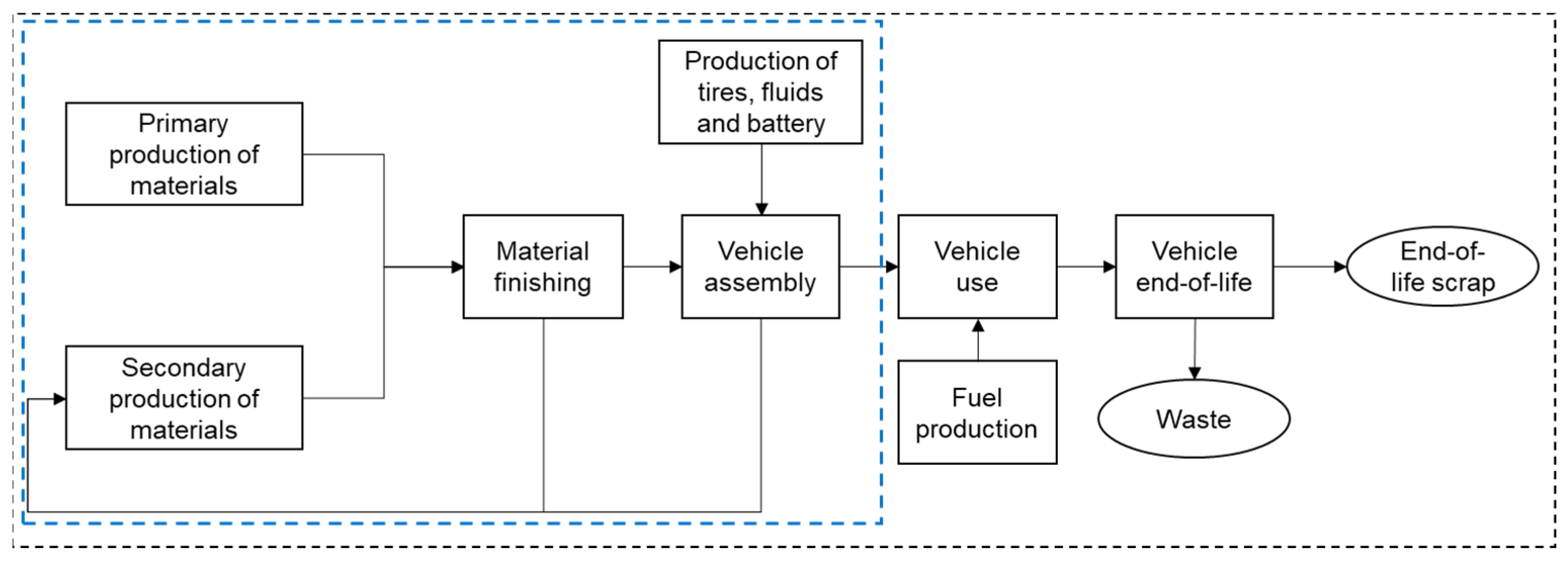
2.1. Overview of the Method

This study deploys the “CO₂ savings” and the “CO₂ payback time” as indicators for the CO₂ benefits. A steel-intensive mid-sized ICEV manufactured in 2010 was considered as the baseline ICEV of the study. Furthermore, aluminum and magnesium were considered as the lightweight materials that substitute for the conventional steel in the above ICEV. The cut-off approach and three commonly used allocation methods for recycling, waste-mining, and 50:50, and end-of-life recycling methods were selected for the evaluation [23] (See Section 2.2 for more details).

Three different natured LCI analyses were conducted centering on the life cycles of steel-, aluminum-, and magnesium-intensive ICEVs (The basic life cycle of an ICEV is depicted in Figure 1) under the respective allocation methods for recycling, as stated above. Those were: (1) A single-ICEV static LCI analysis; (2) Single-ICEV dynamic analyses, with and without dynamic inventory; and (3) Fleet-scale dynamic analyses, with and without dynamic inventory. The average lifetime of an ICEV was set at 12.6 years, as per the lifetime distribution model used in the fleet-scale dynamic LCI analyses herein.

In view of preserving the simplicity in the above LCI analyses, the processing scrap generated during the vehicle assembly was assumed to be internally recycled, and the CO₂ burdens associated with the replacement of tires, fluids, and batteries during vehicle use were neglected. Furthermore, processes demarcated by a blue perforated line in Figure 1 were considered as a single conglomerate, representing the production phase of ICEVs.

Inventories of baseline, aluminum-, and magnesium-intensive ICEVs were calculated following the WorldAutoSteel Energy and GHG Model [47]. The required parameters (i.e., the parameters of the end-of-life recycling method, the fuel economy of the baseline ICEV, and the fuel reduction values for light-weighted ICEVs, required to calculate the use-phase emissions, emission factors, etc.) were established with reference to the literature found on the IDEA, version 2.2 [48], and the Ecoinvent, version 3.5 [49] LCI databases. The CO₂ savings were computed by subtracting the life-cycle CO₂ emissions of the baseline ICEV from those of the respective light-weighted ICEVs under each allocation method. The payback times of the single-ICEV dynamic and fleet-scale dynamic analyses were determined with reference to the cross-over points of the cumulative CO₂ emissions of the baseline and the light-weighted ICEVs under the same (see Table S1 in Supplementary Materials for all parameters used in the study).

2.2. Allocation Approaches and Methods

Materials can be recycled multiple times in a series of product life cycles, generating recycling effects, i.e., burdens avoided, for instance, by consuming the secondary resources from the previous life cycle in the current life cycle. To consider the recycling effects, expanding the system boundary to previous and subsequent product life cycles is necessary. Then, to calculate the LCI of the current life cycle, allocating the recycling effects between the previous, current, and subsequent product life cycles is required. Though this “allocation of recycling effects” is under much debate in the field of life-cycle assessment (LCA), several allocation approaches and methods have already been proposed in the literature [50]. Of them, the commonly used allocation approaches and methods were considered for this study.

2.2.1. The Cut-Off Approach

This approach only accounts for the environmental impacts that are directly related to the functional units of products [23]. In other words, this approach is constrained to the system boundary of the production system itself and tends to neglect the allocation of recycling effects derived from both consuming and recovering secondary resources on the input and output sides of the current life cycle, respectively. The formula for the cut-off approach is defined by Equation (1) [23]:

$$X_{LCI}=X_{pr}-SY\left(X_{pr}-X_{re}\right)+\left(1-R\right)W$$

(1)

where $X_{LCI}$ is the LCI (with recycling effects) of the material used for the current product; $X_{pr}$ is the LCI for primary material production; $X_{re}$ is the LCI for secondary material production; $S$ is the fraction of secondary resources supplied for the material of interest; $Y$ is the process yield; $W$ is the LCI of the waste treatment of the material used for the current product; and $R$ is the fraction of material recovered as secondary resources during the life cycle of the current product.

2.2.2. The Waste-Mining Method

If the market for a secondary resource has shrunk or disappeared, providing the secondary resource will not bring benefits [44,51]. In such cases, the increase in the secondary resource may lead to a decrease in the recovery from other products, and those resources may no longer be treated as resources [50]. Here, a credit created by recycling should be given to the consumption of secondary resources [23]. In this method, no environmental credit is given for recovering secondary resources, and it is modeled as if the end-of-life recycling rate is zero (100% waste disposal); the formula representing the waste-mining method is given in Equation (2) [23]:

$$X_{LCI}=X_{pr}-SY\left(X_{pr}-X_{re}\right)-S{W}_{previous}+W$$

(2)

where $W_{previous}$ is the LCI for the waste treatment of the material used for the previous product.

2.2.3. The End-of-Life Recycling Method

In the end-of-life recycling method, the recycling effects incurred by recovering a secondary resource in the current life cycle is allocated to the current life cycle itself on the premise that this recovered secondary resource avoids the production of primary materials in the subsequent life cycle; however, the consumption of secondary resources in the current life cycle is not credited [23]. The equation for the end-of-life recycling method can be given as Equation (3):

$$X_{LCI}=X_{pr}-RY\left(X_{pr,next}-X_{re, next}\right)+\left(1-R\right)W$$

(3)

where $X_{pr,next}$ and $X_{re,next}$ are the LCIs for primary and secondary material production in the next life cycle.

2.2.4. The 50:50 Method

The 50:50 method shares the credits (generated by consuming and recovering secondary resources in the current life cycle) and the burdens incurred from recycling in the current life cycle with previous and subsequent life cycles; it can be defined as Equation (4). This method is based on the premise that the price elasticity of the supply and demand of the material of interest is equal [50]:

$$X_{LCI}=X_{pr}-0.5SY\left(X_{pr}-X_{re}\right)-0.5S{W}_{previous}-0.5RY\left(X_{pr,next}-X_{re, next}\right)-0.5RW+W$$

(4)

2.3. Material Inventory Calculations

The baseline ICEV herein weighed 1656 kg [47]. The yield ratios at vehicle assembly for steel-, aluminum-, and magnesium-related materials were assumed at 65% [26], while those for the rest of the materials were presumed to be 100%. Moreover, a 0% yield ratio was assumed at the material finishing stage for all materials. The weight of each material at the inventory of the ICEV was divided by the corresponding yield ratio to acquire its unfinished weight on the input side of the “material finishing”.

Conventional steel, weighing 360 kg (i.e., 90% of flat carbon steel and 10% of long and special steel) could be replaced by lightweight materials [52], i.e., wrought aluminum and magnesium. Therefore, the amount required to replace the steel to be removed was calculated by multiplying the aforementioned weight by the material replacement coefficients of aluminum and magnesium. The reduced weight is deemed “primary weight savings”. The savings acquired through the further reduction of materials at the suspension, structural components, transmission, etc., are called “secondary weight savings” [10]. Herein, the secondary weight savings were assumed to be 30% of the primary weight savings. Flat carbon and special steel and wrought and cast aluminum were assumed to have shares of 30, 20, 20, and 30% of the secondary weight savings, respectively. The “weight savings for each material”, thus, could be calculated by adding its primary and secondary weight savings. Bills of the materials of the aluminum-and magnesium-intensive ICEVs were obtained; the final weights of them were recorded at 1485 and 1396 kg, respectively.

2.4. Use-Phase Inventory Calculations

Use-phase-bound CO₂ emissions for the baseline and light-weighted vehicles were calculated following Equations (5) and (6), respectively. The fuel economy, $F_C$, and the fuel reduction values (FRVs) of those equations were determined with reference to Kim et al. [11]. Required emission factors (i.e., gasoline production and combustion) were extracted from the IDEA version 2.2 database [53]. The annual distance traveled was assumed to be 15,000 km and remained constant throughout the lifetime of the ICEVs.

$$X_{use, baseline }=F_C·d\times (E{F}_{gp}+E{F}_{gc})$$

(5)

where $X_{use,baseline}$, $F_C$, $d$, $E{F}_{gp}$, and $E{F}_{gc}$ are the CO₂ emissions from the use phase, the fuel consumption of the standard ICEV, the running distance, and the CO₂ emission factors for gasoline production and combustion, respectively.

$$X_{use, lightweighted }=\left[(F_C·d)-FRV·∆M·d\right]\times (E{F}_{gp}+E{F}_{gc})$$

(6)

where $X_{use,lightweighted}$, $\Delta M$, and $FRV$ are the CO₂ emissions from the use phase of the light-weighted ICEV, the weight change, and the fuel reduction value, respectively.

2.5. Development of Dynamic Inventory

In general, dynamic inventory refers to the temporal variations of the LCI parameters along the period of forecast. To avoid complicacy in preparing the dynamic inventory, the aforementioned variations herein were based on the fluctuations in the CO₂ intensity of the world average electricity grid mix along the forecast period. Parametric variations related to primary aluminum and magnesium (i.e., the Pidgeon process: 70%; the electrolytic process: 30%), plastic, secondary steel (i.e., the electric arc furnace process), and aluminum production were considered for the dynamic inventory. However, considering the lack of inventory data and the dependency on electricity, the rest of the parameters were assumed unchanged along the forecast period. The temporal variation of each LCI parameter was calculated by changing the CO₂ emissions derived from the electricity use per functional unit (within the “overall CO₂ emissions per functional unit”), according to the CO₂ intensity change in the subjected electricity grid mix.

The carbon dioxide intensities of the world average electricity grid mix were extracted from the International Energy Agency’s historical and sustainable development scenario (SDS) data [54]. Because of the absence of CO₂ intensities beyond 2040 in the SDS, the existing CO₂ intensities were extrapolated up to 2060, assuming those will reach 0 kg CO₂ per kWh by 2050.

2.6. Types of Life-Cycle Inventory Analyses

2.6.1. Single-ICEV Static LCI Analyses

The single-ICEV static LCI analysis herein estimates the life cycle CO₂ emissions of a single ICEV and assumes that the life-cycle model parameters remain constant over time; hence, it necessarily “compresses” all time-dependent emissions into a single value, and merely provides a snapshot of the life-cycle CO₂ emissions [14,15]. The single-ICEV static analyses herein are based on the parameters from the year 2010. The CO₂ savings were calculated by subtracting the CO₂ emissions of the baseline ICEV from those of the lightweight ICEVs for each allocation approach.

2.6.2. Single-ICEV Dynamic LCI Analyses

Similar to the single-ICEV static analysis, single-ICEV dynamic analyses belong to the conventional LCI category, as they are based on a single product [15]. In this type of analysis, life-cycle emissions are distributed across time; hence, they provide a more detailed overview of the temporal variations of emissions than its single-ICEV static counterpart. All of the life-cycle stages of the single-ICEV dynamic analyses without dynamic inventory were based in the year 2010, while the production, use, and end-of-life phases of those with dynamic inventory were based in the years, 2010 and 2023, respectively. Paybacks were achieved referring to point “0” of the cumulative CO₂ emission differences (i.e., the crossover points of the cumulative CO₂ emissions of the baseline and the respective light-weighted ICEVs) of each light-weighted ICEV under the respective allocation method. The time series change of the CO₂ savings is represented by the cumulative CO₂ emission difference curve belonging to each allocation method.

2.6.3. Fleet-Scale Dynamic LCI Analyses

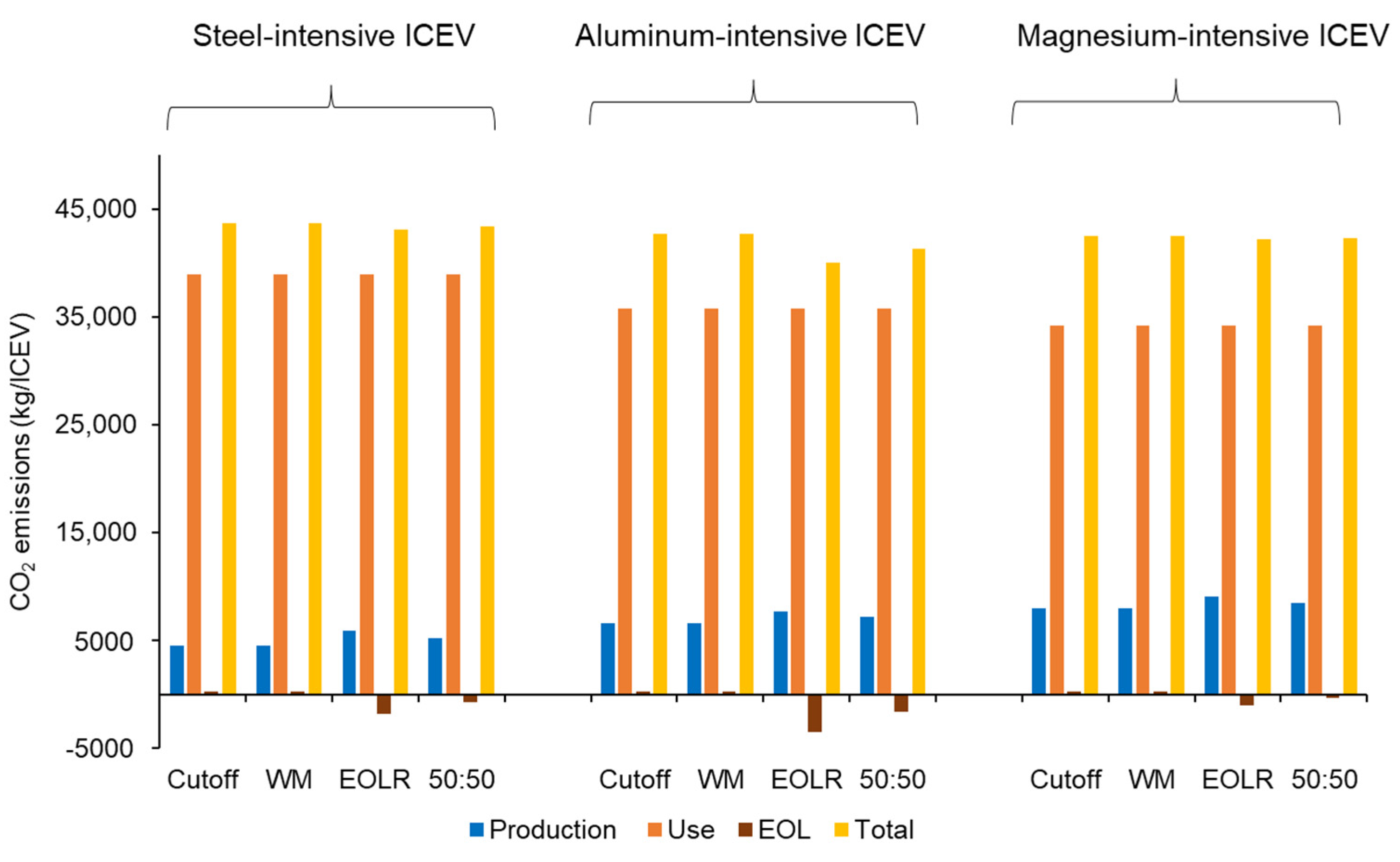
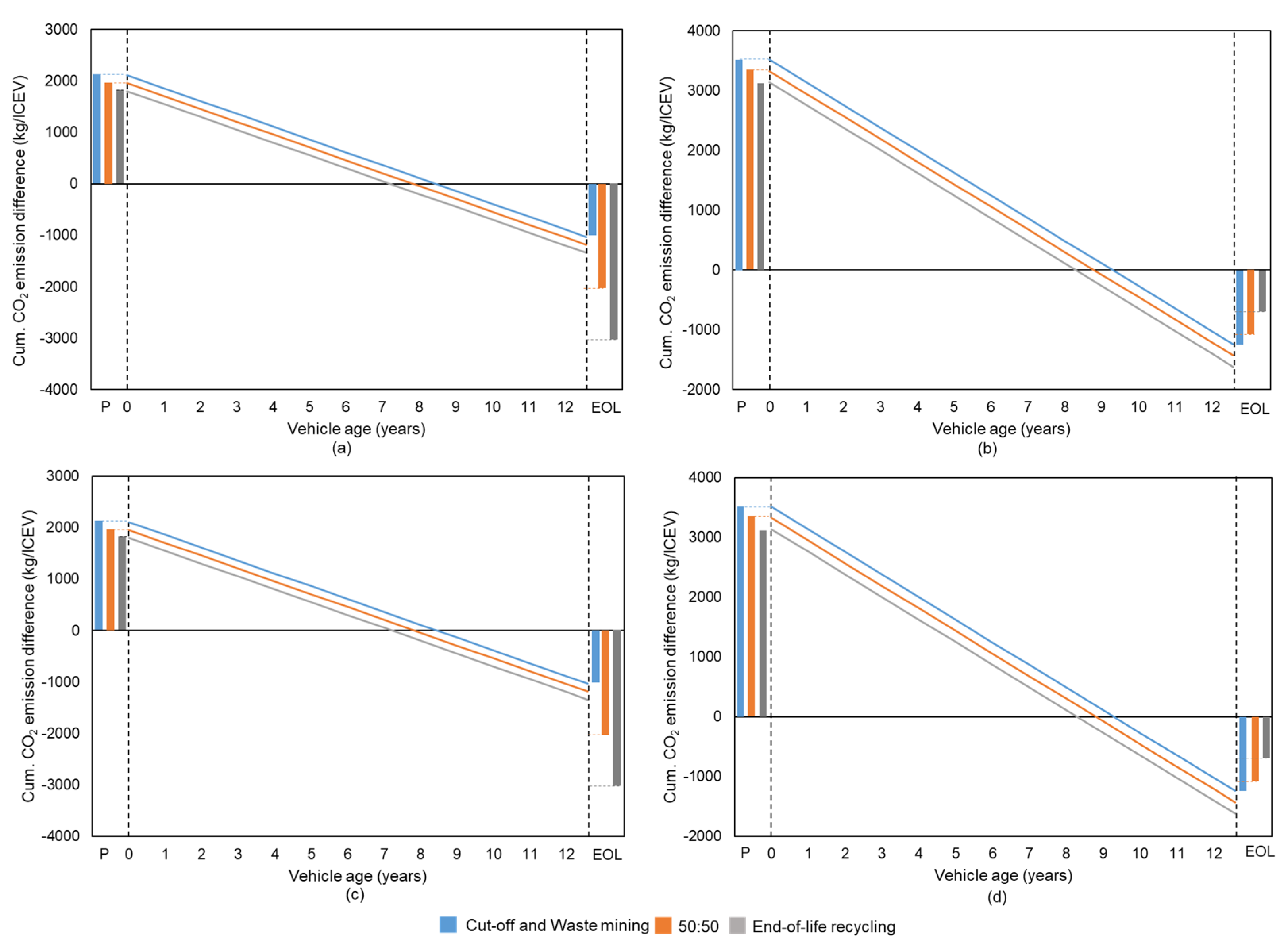
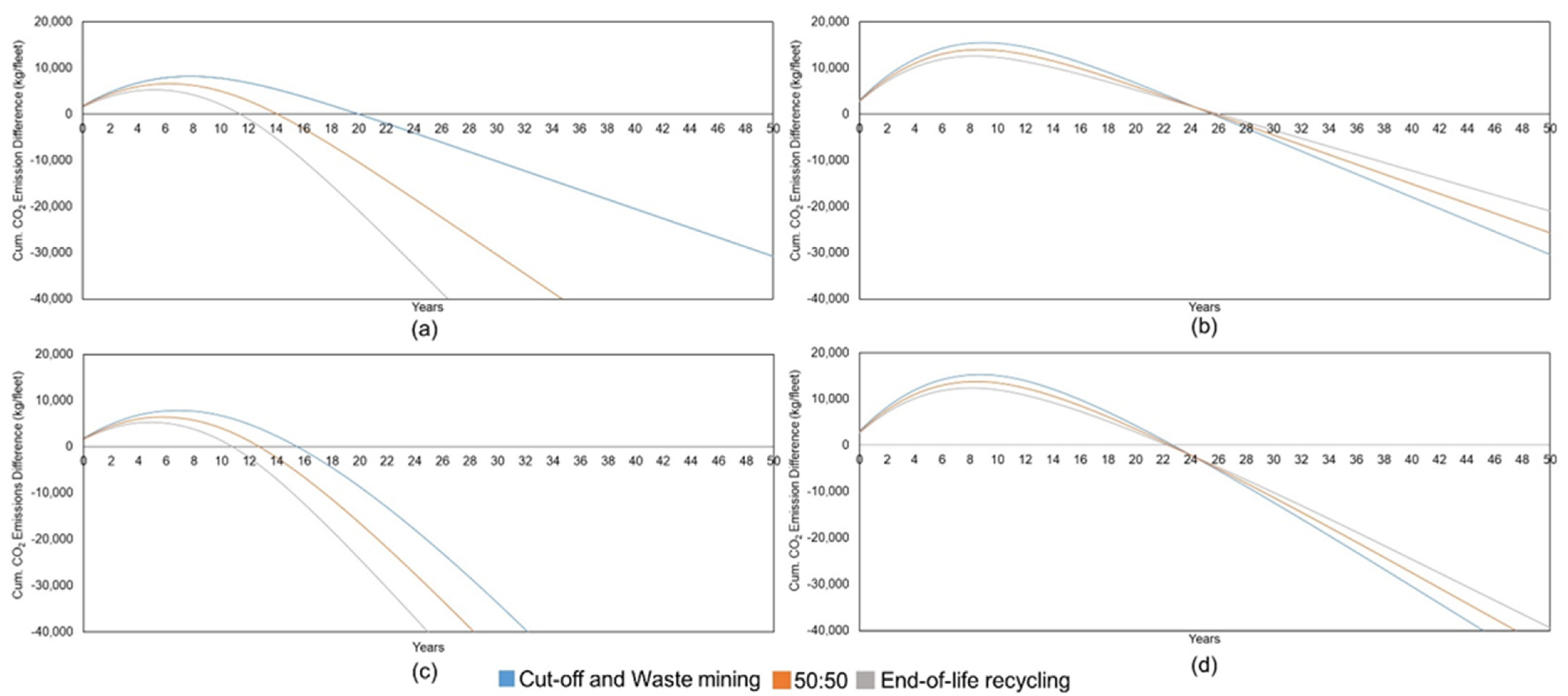
Fleet analyses account for changes over time in the CO₂ emissions in a vehicle fleet using a fleet model that accounts for the dynamics of vehicle introduction and the scrappage rates in each year [14,43,55]. Since the objective here is to investigate the behavior of the payback times of ICEVs with new material types, the start of the analysis is a zero-car fleet that grows at a fixed rate annually during the forecast period, i.e., 50 years [40,41]. A single unit of vehicle is assumed to be produced each year for simplicity, as it could be any multiple of any sales figure. Furthermore, a flat annual growth rate of the ICEVs (i.e., one unit is produced and added to the “units in service” annually) was assumed to preserve the simplicity in the calculations. The fleet model was constructed following the lifetime distribution model for ICEVs in Daigo et al. [55]. The payback times for each light-weighted ICEV were acquired for each allocation method by referring to the point “0” of the cumulative CO₂ emission differences. The cumulative CO₂ emission difference curve represents the time-series change of the CO₂ savings for each allocation method.

3. Results

Figure 2 illustrates the life-cycle CO₂ emissions of baseline, aluminum-, and magnesium-intensive cars, acquired using the cut-off approach, and the waste-mining, end-of-life recycling, and 50:50 methods for single-car static analyses. As per Figure 2, the use-phase emissions dominated the overall emissions of baseline, aluminum-, and magnesium-intensive cars. Since the recovery rates assumed for flat carbon, long special steel, and wrought aluminum are larger than their recycled contents, avoided burdens from recovering secondary resources under the end-of-life recycling and 50:50 methods have become larger than those from consuming secondary resources under the cut-off approach and the waste-mining method in the case of aluminum-intensive ICEVs. As a result, CO₂ emissions recorded under the cut-off approach and the waste-mining method become larger than those under the end-of-life recycling and 50:50 methods for that ICEV. On the other hand, the magnesium’s recycled content and end-of-life recycling rates were assumed to be 0% for this study. Hence, total avoided burdens from recovering secondary resources (under the end-of-life recycling and 50:50 methods) have become smaller than those from consuming secondary resources (under the cut-off approach and waste-mining method) for magnesium-intensive ICEVs; this has made CO₂ emissions under the end-of-life recycling and 50:50 methods larger than those computed under the cut-off approach and the waste-mining method. Furthermore, both light-weighted ICEVs have yielded CO₂ savings at each allocation method, indicating the possibility of CO₂ payback times.

Figure 3 depicts the CO₂ savings and payback times of single-ICEV dynamic analyses for both aluminum- and magnesium-intensive ICEVs, with and without dynamic inventory. In all cases, the CO₂ payback times appear during the use phase and tend to vary across the allocation methods, i.e., the shortest payback period is from end-of-life recycling, while the second shortest, and the longest, are from the 50:50 method, the cut-off approach, and the waste-mining method, respectively. The difference of the avoided burdens from consuming secondary resources at the baseline ICEV remain larger than those from the aluminum- and magnesium-intensive ICEVs. Zeroed recycled contents of wrought aluminum and magnesium are the main factors for the lowered avoided burdens. Hence, the emission offsets under the cut-off approach and the waste-mining method were more delayed than those under the 50:50 and end-of-life recycling methods for those vehicles.

According to Figure 3a,b, the CO₂ savings for the magnesium-intensive ICEV under the cut-off approach and the waste-mining method have become larger than those for the aluminum-intensive ICEV under the same. Furthermore, the largest CO₂ savings are visible in the cut-off approach and the waste-mining method for the magnesium-intensive ICEV. The influence of CO₂ credits from the uplifted fuel economy and the zeroed avoided burdens from the recovery of secondary resources of magnesium in the end-of-life recycling and 50:50 methods are the roots of such trends. At this juncture, one who uses the cut-off approach or the waste-mining method may select magnesium over aluminum, while someone else who uses the end-of-life recycling or the 50:50 methods does vice versa. Therefore, material selection using CO₂ savings can differ from that implemented using payback times under single-ICEV dynamic analyses.

However, according to Figure 3c,d, the inclusion of the dynamic inventory has altered neither the payback times nor the CO₂ savings for both aluminum- and magnesium-intensive ICEVs for the following reasons: (1) Paybacks occurred during the use phase, the parameters of which remain unchanged; and (2) The changes that the dynamic inventory gives to the end-of-life phase of the respective ICEV are negligible.

Figure 4 encapsulates the figures for the time-series changes of the CO₂ savings and payback times under fleet-scale dynamic LCI analyses, in the presence and absence of dynamic inventory, for both aluminum- and magnesium-intensive fleets. In Figure 4a,b in which the dynamic inventory is not included, all payback times for both vehicles were delayed, unlike those indicated under single-ICEV dynamic LCI analyses. However, at all allocation methods, the aluminum-intensive ICEV tends to perform better than the magnesium-intensive ICEV, resembling the results of the corresponding single-ICEV dynamic analyses. In general, delays in payback times can occur because of the nature of the fleet model; in the fleet model, fresh units are introduced in the early years, allowing production-based CO₂ emissions to dominate in the early stages. Since no CO₂ emission credits can be expected from the production phase of the lightweight ICEVs (i.e., aluminum- and magnesium-intensive ICEVs), CO₂ emission gaps between the baseline and respective lightweight fleets tend to get larger during the early years.

The behavior of the payback times for the magnesium-intensive fleet is different from that of the aluminum-intensive fleet, where the curves converge before reaching the breakeven points; this has given the cut-off approach, and the waste-mining and EOLR methods the shortest and longest payback times, respectively. Convergence here reflects the weakened effect of the end-of-life phases of the end-of-life recycling and 50:50 methods, where the avoided burdens from recovering secondary resources of magnesium are zero. In this case, unlike the CO₂ payback times observed in the single-ICEV dynamic analyses, those observed in the fleet-scale dynamic LCI analyses were influenced by the CO₂ emissions associated with the EOL phase.

Carbon dioxide savings seem to depend on the “period of forecast” in fleet-scale dynamic LCI analyses. For instance, the CO₂ savings computed in the cut-off and waste-mining methods for both aluminum- and magnesium-intensive ICEVs are almost the same for the 50-year period of the forecast (see Figure 4a,b). Therefore, an intersection of them can be expected when a longer period of forecast than 50 years is considered; this means that the CO₂ savings of magnesium-intensive ICEVs become larger than those of aluminum-intensive ICEVs. Therefore, the material being selected, using CO₂ savings in the cut-off approach or the waste-mining method, can be different from that being selected with reference to the CO₂ payback times at the same under a fleet-scale dynamic analysis with a longer period of forecast.

Figure 4c,d depict the payback times for aluminum- and magnesium-intensive fleets in the presence of dynamic inventory, respectively. With the introduction of dynamic inventory, all of the payback times of aluminum- and magnesium-intensive ICEVs have been shortened; this stems from the reduction in the CO₂ emissions of primary aluminum and magnesium production during the forecast period (see Figure S1 in Supplementary Materials). The CO₂ emissions attributed to primary aluminum production heavily depend on the electricity consumption of the smelting process; hence, reducing the CO₂ intensity of the electricity grid mix along the period of forecast alleviated the overall CO₂ emissions of primary aluminum production by a significant amount. The Pidgeon process, which is the main process to produce magnesium, is less dependent on electricity, unlike its counterpart, the electrolytic process; hence, relatively fewer CO₂ reductions are evident.

4. Discussion

As per the results, the aluminum-intensive ICEV always performed better than the magnesium-intensive ICEV in the respective allocation methods for recycling, while the dynamic inventory was highly sensitive to the CO₂ savings and payback times calculated under the fleet-based LCI analyses.

However, the inclusion of a dynamic inventory that captures more aspects, such as the production ratio of the Pidgeon process, future possibilities for recycling magnesium as a structural material, etc., results in shorter payback time(s) for magnesium-intensive ICEVs in certain allocation method(s) for recycling. See Figure 5, where the payback periods for the magnesium-intensive ICEV in the cut-off approach and the waste mining method are shorter than those of the aluminum-intensive ICEV. Therefore, in the absence of such a dynamic inventory, the payback time of aluminum under a particular allocation method will always be shorter than that of magnesium under fleet-scale dynamic LCI analyses; moreover, such a variation will not be reflected either through single-ICEV static or dynamic analyses. Hence, conducting fleet-scale dynamic LCI analyses with a dynamic inventory can be pivotal in knowing the payback times.

With the addition of dynamic inventory, the CO₂ savings of the aluminum-intensive fleet under the cut-off approach and other allocation methods have become larger than those of the magnesium-intensive fleet, regardless of the “period of forecast”, as no intersection of the curves is evident or can be imagined within or beyond the 50-year forecast period considered herein (see Figure 4c,d). However, a dynamic inventory that captures more aspects can bring back the “influence of period of forecast”, i.e., the possibility of different materials being selected at different periods of forecasts under the exact allocation method (see Figure 5, where CO₂ savings under each allocation method for the magnesium-intensive ICEV are larger than those for the aluminum-intensive ICEV within the subjected period of forecast). Therefore, this implies that conducting a fleet-scale dynamic LCI analysis, including a dynamic inventory, is important in knowing the CO₂ savings for material selections.

However, if magnesium has higher recycled content than its end-of-life recycling rate, it can result in shorter payback times in the cut-off approach and the waste-mining method (see Figure 6), while aluminum with a lower recycled content than its end-of-life recycling rate indicates shorter payback times in the EOLR and 50:50 methods. Hence, a practitioner using the 50:50 or end-of-life recycling methods would select the aluminum-intensive ICEV as the best choice, while someone else using the cut-off approach or the waste-mining method would select the magnesium-intensive ICEV as the best option. Hence, the choice of allocation method can perform a salient role in the payback time evaluations in fleet-based LCI dynamic analyses.

The same tendency is evident in the CO₂ savings. If magnesium possesses larger recycled content than the end-of-life recycling rate, it can show larger CO₂ savings in the cut-off approach and the waste-mining method, regardless of the period of forecast (see Figure 6). However, in the case of aluminum, the end-of-life recycling rate is larger than the recycled content; hence, larger CO₂ savings are observable in the 50:50 and end-of-life recycling methods, regardless of the same. In short, upon the selection of the allocation method, the material being selected can vary; hence, the choice of allocation approach is deemed important in terms of material selection using CO₂ savings.

Overall, the choice of allocation method and conducting fleet-based dynamic LCI analyses under the presence of dynamic inventory were critical in obtaining the CO₂ savings or payback times for consistent and accurate material selections.

The payback times and the CO₂ savings are sensitive to the kind of data that is referred to when determining the $X_{pr}$ and $X_{re}$, the recycled contents, the end-of-life recycling rates, the material substitution rates, the annual distance traveled, the fuel reduction value, and the secondary mass reduction rate, along the period of forecast representing dynamic inventory. Hence, in order to achieve consistent payback times, regardless of the time and place of evaluation, a common dataset is required for the above parameters. However, predicting such parameters can be difficult, as the future is uncertain. Approaches, such as dynamic material flow analysis [56] and scenario modeling [57], may be helpful in this regard.

As mentioned earlier, a designated methodology or criteria for selecting an allocation method for recycling has been absent, except for methods relying upon market information that is highly changeable and infrequently documented; hence, a more convenient method that depends on less changeable and more readily accessible information is required for the above selection process. For instance, a methodology that refers to material properties can be a solution, as the material properties are less vulnerable to rapid fluctuations.

According to the pressure that climate change has put on manufacturers, they are required to provide products with smaller carbon footprints across life cycles to the market. At the initial stage, manufacturers decide on a design for their products, which significantly affects the footprint. One of the issues in the design phase is material selection. This paper successfully demonstrates a case study that proved that conventional LCI analyses might lead to the wrong choice of materials. According to this study, we recommend that manufacturers conduct an inventory analysis at the fleet scale, formulate a certain reason for selecting the allocation method of recycling, and perform a dynamic inventory, considering the lifespan of their products, in order to make better choices of materials.

Furthermore, the carbon footprint is not the only target for sustainability. In many cases, a decision causes tradeoffs between different categories of environmental impacts. In the context of the LCA, some approaches have been proposed for harmonizing different impact categories: environmental priority strategies in product development [58], distance-to-target [59], the panel method [60], and the analytic hierarchy process [61,62].

5. Conclusions

We highlight the importance of the choice of allocation method for recycling and conducting fleet-scale dynamic analyses in the presence of dynamic inventory for material selections through an LCI case study on aluminum- and magnesium- substituted ICEVs.

Aluminum-intensive ICEVs always performed better than magnesium-intensive ICEVs (with larger CO₂ savings and shorter payback times) in the respective allocation methods for recycling, regardless of the presence of the subjected dynamic inventory (based on the change in the world average electricity grid mix) under fleet-based LCI analyses. However, we identified that a dynamic inventory capturing more aspects could make magnesium-intensive ICEVs perform better than others in certain allocation method(s) for recycling under the same.

Furthermore, when the recycled content of magnesium was greater than its recovery rate, magnesium-intensive ICEVs resulted in larger CO₂ savings and shorter payback times in certain allocation methods under fleet-based analyses. Such instances could compel practitioners to select magnesium-intensive ICEVs over others in those allocation methods for recycling.

Therefore, the choice of the allocation method for recycling and the execution of fleet-based dynamic LCI analyses under the presence of dynamic inventory are crucial in obtaining the CO₂ savings or payback times for material selections. Neglecting even one of them may result in the wrong material selection. Standardizing the selection of the allocation methods for recycling and a common dataset for the dynamic inventory are dire requirements for assuring accordance in the calculations of the CO₂ savings and payback times, regardless of the time and place of the evaluations.

References

1. Koncar, V. Introduction to smart textiles and their applications. In Smart Textiles and Their Applications; Woodhead Publishing Ltd.: Oxford, UK, 2016; pp. 1–8. [Google Scholar] [CrossRef]
2. European Union. Blending in the Transport Sector. Available online: http://bookshop.europa.eu (accessed on 2 March 2021).
3. Sussman, R.; Tan, L.Q.; Kormos, C.E. Behavioral interventions for sustainable transportation: An overview of programs and guide for practitioners. In Transport and Energy Research; Elsevier: Amsterdam, The Netherlands, 2020; pp. 315–371. [Google Scholar]
4. Hossain, M.F. Sustainable Design and Build: Building, Energy, Roads, Bridges, Water and Sewer Systems; Butterworth-Heinemann: Oxford, UK, 2018; ISBN 978-0-12-816888-2. [Google Scholar]
5. Ritchie, H.; Roser, M. Global Greenhouse Gas Emissions by Sector. Available online: https://ourworldindata.org/emissions-by-sector (accessed on 18 October 2021).
6. National Institute for Environmental Studies. Greenhouse Gas Inventory Office of Japan. Available online: http://www.nies.go.jp/gio/en/index.html (accessed on 18 October 2021).
7. European Commission. Commission and ACEA Agree on CO2 Emissions from Cars. Available online: https://ec.europa.eu/commission/presscorner/detail/en/IP_98_734 (accessed on 18 October 2021).
8. The European Automobile Manufacturers’ Association. Publications. Available online: https://www.acea.auto/nav/?content=publications (accessed on 18 October 2021).
9. Directorate-General for Climate Action (European Commission); Ricardo Energy & Environment; Hill, N.; Amaral, S.; Morgan-Price, S.; Nokes, T.; Bates, J.; Helms, H.; Fehrenbach, H.; Biemann, K.; et al. Determining the Environmental Impacts of Conventional and Alternatively Fuelled Vehicles through LCA: Final Report; Publications Office of the European Union: Luxembourg, 2020. [Google Scholar]
10. Kim, H.-J.; McMillan, C.; Keoleian, G.A.; Skerlos, S.J. greenhouse gas emissions payback for lightweighted vehicles using aluminum and high-strength steel. J. Ind. Ecol. 2010, 14, 929–946. [Google Scholar] [CrossRef]
11. Kim, H.C.; Wallington, T.J.; Sullivan, J.L.; Keoleian, G.A. Life Cycle Assessment of Vehicle Lightweighting: Novel Mathematical Methods to Estimate Use-Phase Fuel Consumption. Environ. Sci. Technol. 2015, 49, 10209–10216. [Google Scholar] [CrossRef]
12. Kim, H.C.; Wallington, T.J. Life Cycle Assessment of vehicle lightweighting: A physics-based model to estimate use-phase fuel consumption of electrified vehicles. Environ. Sci. Technol. 2016, 50, 11226–11233. [Google Scholar] [CrossRef] [PubMed]
13. Hottle, T.; Caffrey, C.; McDonald, J.; Dodder, R. Critical factors affecting life cycle assessments of material choice for vehicle mass reduction. Transp. Res. Part D Transp. Environ. 2017, 56, 241–257. [Google Scholar] [CrossRef] [PubMed]
14. Garcia, R.; Freire, F. A review of fleet-based life-cycle approaches focusing on energy and environmental impacts of vehicles. Renew. Sustain. Energy Rev. 2017, 79, 935–945. [Google Scholar] [CrossRef]
15. Kirchain, R. Fleet-Based LCA: Comparative CO2 Emission Burden of Aluminum and Steel Fleets. Available online: https://dspace.mit.edu/handle/1721.1/1405 (accessed on 18 October 2021).
16. Thomassen, M.A.; Dalgaard, R.; Heijungs, R.; de Boer, I. Attributional and consequential LCA of milk production. Int. J. Life Cycle Assess. 2008, 13, 339–349. [Google Scholar] [CrossRef] [Green Version]
17. Del Pero, F.; Delogu, M.; Pierini, M. Life Cycle Assessment in the automotive sector: A comparative case study of Internal Combustion Engine (ICE) and electric car. Procedia Struct. Integr. 2018, 12, 521–537. [Google Scholar] [CrossRef]
18. Kawamoto, R.; Mochizuki, H.; Moriguchi, Y.; Nakano, T.; Motohashi, M.; Sakai, Y.; Inaba, A. Estimation of CO2 Emissions of Internal Combustion Engine Vehicle and Battery Electric Vehicle Using LCA. Sustainability 2019, 11, 2690. [Google Scholar] [CrossRef] [Green Version]
19. Schaubroeck, T.; Schaubroeck, S.; Heijungs, R.; Zamagni, A.; Brandão, M.; Benetto, E. Attributional & Consequential Life Cycle Assessment: Definitions, Conceptual Characteristics and Modelling Restrictions. Sustainability 2021, 13, 7386. [Google Scholar] [CrossRef]
20. Fantozzi, F.; Bartocci, P.; D’Alessandro, B.; Testarmata, F. Carbon footprint of truffle sauce in central Italy by direct measurement of energy consumption of different olive harvesting techniques. J. Clean. Prod. 2015, 87, 188–196. [Google Scholar] [CrossRef]
21. Weis, A.; Jaramillo, P.; Michalek, J. Consequential life cycle air emissions externalities for plug-in electric vehicles in the PJM interconnection. Environ. Res. Lett. 2016, 11, 024009. [Google Scholar] [CrossRef]
22. Palazzo, J.; Geyer, R. Consequential life cycle assessment of automotive material substitution: Replacing steel with aluminum in production of north American vehicles. Environ. Impact Assess. Rev. 2019, 75, 47–58. [Google Scholar] [CrossRef]
23. Schrijvers, D.L.; Loubet, P.; Sonnemann, G. Developing a systematic framework for consistent allocation in LCA. Int. J. Life Cycle Assess. 2016, 21, 976–993. [Google Scholar] [CrossRef]
24. Suzuki, T.; Odai, T.; Hukui, R. LCA of Passenger Vehicles Lightened by Recyclable Carbon Fiber Reinforced Plastics; University of Tokyo: Tokyo, Japan, 2005. [Google Scholar]
25. Moon, P.; Burnham, A.; Wang, M. Vehicle-Cycle Energy and Emission Effects of Conventional and Advanced Vehicles; SAE International: Warrendale, PA, USA, 2006. [Google Scholar]
26. Hakamada, M.; Furuta, T.; Chino, Y.; Chen, Y.; Kusuda, H.; Mabuchi, M. Life cycle inventory study on magnesium alloy substitution in vehicles. Energy 2007, 32, 1352–1360. [Google Scholar] [CrossRef]
27. Tharumarajah, A.; Koltun, P. Is there an environmental advantage of using magnesium components for light-weighting cars? J. Clean. Prod. 2007, 15, 1007–1013. [Google Scholar] [CrossRef]
28. Tharumarajah, A.; Koltun, P. Improving environmental performance of magnesium instrument panels. Resour. Conserv. Recycl. 2010, 54, 1189–1195. [Google Scholar] [CrossRef]
29. Kelly, J.C.; Sullivan, J.L.; Burnham, A.; Elgowainy, A. Impacts of Vehicle Weight Reduction via Material Substitution on Life-Cycle Greenhouse Gas Emissions. Environ. Sci. Technol. 2015, 49, 12535–12542. [Google Scholar] [CrossRef] [PubMed]
30. Du, J.; Han, W.; Peng, Y.; Gu, C. Potential for reducing GHG emissions and energy consumption from implementing the aluminum intensive vehicle fleet in China. Energy 2010, 35, 4671–4678. [Google Scholar] [CrossRef]
31. Ribeiro, I.; Peças, P.; Silva, A.; Henriques, E. Life cycle engineering methodology applied to material selection, a fender case study. J. Clean. Prod. 2008, 16, 1887–1899. [Google Scholar] [CrossRef]
32. Bertram, M.; Buxmann, K.; Furrer, P. Analysis of greenhouse gas emissions related to aluminium transport applications. Int. J. Life Cycle Assess. 2009, 14, 62–69. [Google Scholar] [CrossRef]
33. Puri, P.; Compston, P.; Pantano, V. Life cycle assessment of Australian automotive door skins. Int. J. Life Cycle Assess. 2009, 14, 420–428. [Google Scholar] [CrossRef]
34. Das, S. Life Cycle Assessment of Carbon Fiber-Reinforced Polymer Composites. Int. J. Life Cycle Assess. 2011, 16, 268–282. [Google Scholar] [CrossRef]
35. Baroth, A.; Karanam, S.; McKay, R. Life Cycle Assessment of Lightweight Noryl* GTX* Resin Fender and Its Comparison with Steel Fender; SAE International: Warrendale, PA, USA, 2012. [Google Scholar]
36. Dhingra, R.; Das, S. Life cycle energy and environmental evaluation of downsized vs. lightweight material automotive engines. J. Clean. Prod. 2014, 85, 347–358. [Google Scholar] [CrossRef]
37. Mayyas, A.; Qattawi, A.; Mayyas, A.R.; Omar, M. Life cycle assessment-based selection for a sustainable lightweight body-in-white design. Energy 2012, 39, 412–425. [Google Scholar] [CrossRef]
38. Dubreuil, A.; Bushi, L.; Das, S.; Tharumarajah, A.; Gong, X. A Comparative Life Cycle Assessment of Magnesium Front End Autoparts: A Revision to 2010-01-0275; SAE International: Warrendale, PA, USA, 2012. [Google Scholar]
39. Das, S. The life-cycle impacts of aluminum body-in-white automotive material. JOM 2000, 52, 41–44. [Google Scholar] [CrossRef]
40. Das, S. Life cycle energy impacts of automotive liftgate inner. Resour. Conserv. Recycl. 2005, 43, 375–390. [Google Scholar] [CrossRef]
41. Field, F.; Kirchain, R.; Clark, J. Life-Cycle Assessment and Temporal Distributions of Emissions: Developing a Fleet-Based Analysis. J. Ind. Ecol. 2000, 4, 71–91. [Google Scholar] [CrossRef] [Green Version]
42. Cáceres, C.H. Transient environmental effects of light alloy substitutions in transport vehicles. Mater. Des. 2009, 30, 2813–2822. [Google Scholar] [CrossRef]
43. Stasinopoulos, P.; Compston, P.; Newell, B.; Jones, H.M. A system dynamics approach in LCA to account for temporal effects—A consequential energy LCI of car body-in-whites. Int. J. Life Cycle Assess. 2012, 17, 199–207. [Google Scholar] [CrossRef]
44. Weidema, B. Avoiding Co-Product Allocation in Life-Cycle Assessment. J. Ind. Ecol. 2000, 4, 11–33. [Google Scholar] [CrossRef]
45. Levasseur, A.; Lesage, P.; Margni, M.; Deschênes, L.; Samson, R. Considering Time in LCA: Dynamic LCA and Its Application to Global Warming Impact Assessments. Environ. Sci. Technol. 2010, 44, 3169–3174. [Google Scholar] [CrossRef]
46. Collinge, W.O.; Landis, A.E.; Jones, A.K.; Schaefer, L.A.; Bilec, M.M. Dynamic life cycle assessment: Framework and application to an institutional building. Int. J. Life Cycle Assess. 2013, 18, 538–552. [Google Scholar] [CrossRef]
47. Geyer, R. UCSB Energy & GHG Model-WorldAutoSteel. Available online: https://www.worldautosteel.org/life-cycle-thinking/ucsb-energy-ghg-model/ (accessed on 18 October 2021).
48. IDEA. Available online: http://idea-lca.com/?lang=en (accessed on 18 October 2021).
49. Ecoinvent. Ecoinvent Database. Available online: https://ecoinvent.org/the-ecoinvent-database/ (accessed on 18 October 2021).
50. Ekvall, T. A market-based approach to allocation at open-loop recycling. Resour. Conserv. Recycl. 2000, 29, 91–109. [Google Scholar] [CrossRef]
51. European CommissionInternational Reference Life Cycle Data System (ILCD) Handbook-General Guide for Life Cycle Assessment-Detailed Guidance. Available online: https://eplca.jrc.ec.europa.eu/uploads/ILCD-Handbook-General-guide-for-LCA-DETAILED-GUIDANCE-12March2010-ISBN-fin-v1.0-EN.pdf (accessed on 18 October 2021).
52. Geyer, R. Life Cycle Energy and Greenhouse Gas (GHG) Assessments of Automotive Material Substitution User Guide for Version 5 of the UCSB Automotive Energy and GHG Model. Available online: https://www.worldautosteel.org/download_files/UCSB/User%20Guide%20Version%205.pdf (accessed on 18 October 2021).
53. AIST. Inventory Database (IDEAv2). Available online: https://www.aist-riss.jp/softwares/40166/ (accessed on 30 October 2020).
54. IEA. Tracking Power. 2020. Available online: https://www.iea.org/reports/tracking-power-2020 (accessed on 30 October 2020).
55. Daigo, I.; Iwata, K.; Ohkata, I.; Goto, Y. Macroscopic evidence for the hibernating behavior of materials stock. Environ. Sci. Technol. 2015, 49, 8691–8696. [Google Scholar] [CrossRef] [PubMed] [Green Version]
56. Daigo, I.; Osako, S.; Adachi, Y.; Matsuno, Y. Time-series analysis of global zinc demand associated with steel. Resour. Conserv. Recycl. 2014, 82, 35–40. [Google Scholar] [CrossRef]
57. Greiner, R.; Puig, J.; Huchery, C.; Collier, N.; Garnett, S.T. Scenario modelling to support industry strategic planning and decision making. Environ. Model. Softw. 2014, 55, 120–131. [Google Scholar] [CrossRef] [Green Version]
58. Steen, B. A Systematic Approach to Environmental Priority Strategies in Product Development (EPS) Version 2000-Models and Data of the Default Method; Centre for Environmental Assessment of Products and Material Systems: Gothenburg, Sweden, 1999. [Google Scholar]
59. Castellani, V.; Benini, L.; Sala, S.; Pant, R. A distance-to-target weighting method for Europe 2020. Int. J. Life Cycle Assess. 2016, 21, 1159–1169. [Google Scholar] [CrossRef] [Green Version]
60. Volkwein, S.; Gihr, R.; Klöpffer, W. The valuation step within LCA. Int. J. Life Cycle Assess. 1996, 1, 182–192. [Google Scholar] [CrossRef]
61. AlArjani, A.; Modibbo, U.M.; Ali, I.; Sarkar, B. A new framework for the sustainable development goals of Saudi Arabia. J. King Saud Univ. Sci. 2021, 33, 101477. [Google Scholar] [CrossRef]
62. Omair, M.; Noor, S.; Tayyab, M.; Maqsood, S.; Ahmed, W.; Sarkar, B.; Habib, M.S. the selection of the sustainable suppliers by the development of a decision support framework based on analytical hierarchical process and fuzzy inference system. Int. J. Fuzzy Syst. 2021, 23, 1986–2003. [Google Scholar] [CrossRef]
Figure 1. The basic life cycle of an internal combustion engine vehicle. Black and blue perforated lines represent the basic system boundary, and the conglomerate of the production phase processes, respectively.
Sustainability 13 13935 g001
Figure 2. Results of single-ICEV static analyses for baseline, aluminum-, and magnesium-ICEVs.
Sustainability 13 13935 g002
Figure 3. Carbon dioxide savings and payback times of single-car dynamic analyses. (a) Aluminum-intensive ICEV without dynamic inventory; (b) magnesium-intensive ICEV without dynamic inventory; (c) aluminum-intensive ICEV with dynamic inventory; and (d) magnesium-intensive ICEV with dynamic inventory. P and EOL refer to the production and end-of-life phases, respectively.
Sustainability 13 13935 g003
Figure 4. Time-series changes in CO2 savings and CO2 payback times of fleet-scale dynamic LCI analyses. (a) Aluminum-intensive fleet without dynamic inventory; (b) magnesium-intensive fleet without dynamic inventory; (c) aluminum-intensive fleet with dynamic inventory; and (d) magnesium-intensive fleet with dynamic inventory.
Sustainability 13 13935 g004
Figure 5. Payback times and time-series change in CO2 savings under fleet-scale dynamic analyses with dynamic inventory. Aluminum- and magnesium-intensive fleets are represented by continuous and perforated lines, respectively. It was assumed that the production ratio of the Pidgeon process would be 0% by 2020.
Sustainability 13 13935 g005
Figure 6. Payback times and time-series change in CO2 savings under fleet analyses with dynamic inventory. Aluminum- and magnesium-intensive fleets are represented by continuous and perforated lines, respectively. It was assumed that the magnesium’s recycled content and the end-of-life recycling rate were 10% and 5%, respectively.
Sustainability 13 13935 g006