Abstract
The emission estimation of the oil and gas sector, which involves field test measurements, data analysis, and uncertainty estimation, precedes effective emission mitigation actions. A systematic comparison and summary of these technologies and methods are necessary to instruct the technology selection and for uncertainty improvement, which is not found in existing literature. In this paper, we present a review of existing measuring technologies, matching data analysis methods, and newly developed probabilistic tools for uncertainty estimation and try to depict the process for emission estimation. Through a review, we find that objectives have a determinative effect on the selection of measurement technologies, matching data analysis methods, and uncertainty estimation methods. And from a systematic perspective, optical instruments may have greatly improved measurement accuracy and range, yet data analysis methods might be the main contributor of estimation uncertainty. We suggest that future studies on oil and gas methane emissions should focus on the analysis methods to narrow the uncertainty bond, and more research on uncertainty generation might also be required.
1. Introduction
At present, methane is the second largest greenhouse gas in the world, accounting for 20% of global greenhouse gas emissions [1]. It is a strong, short-lived greenhouse gas [2,3], having an indirect impact on human health and affecting the decomposition of some substances in the atmosphere during the process of decaying [4]. Methane emitted by energy activities accounts for about 20% of the anthropogenic methane emissions, the emission of the oil and gas sector accounts for the majority of the methane produced by energy activities [5]. Methane emission reduction prevents the negative climate effect of methane as a “low carbon fuel”, cuts down the global carbon intensity [6,7,8,9], contributes to the achievement of climate goals [10,11,12], and brings about a cobenefit in the economy, public health, and other fields [13,14,15]. As a result, the importance of mitigating methane emission from oil and gas has become increasingly prominent and has widely concerned the international community.
To better manage methane emissions, it is necessary to establish a deep understanding of the total amount of methane emission of different stages in the oil and gas supply chain. Estimations of methane emissions are provided, and three kinds of activities are usually performed in the estimation process: field test measurements to obtain raw data of methane emission sources, data analyses to calculate the emission rate, and uncertainty estimations to evaluate the credibility of the estimation results. The above three activities are conducted separately and sequentially. In recent years, advanced technologies and data analysis methods have been developed and applied to improve the estimation accuracy and lower the uncertainty. Studies also showed that certain kinds of measurement technologies, data analysis methods, and uncertainty estimation methods were often applied together. This is because the application of data analysis methods requires certain kinds of technologies and uncertainty estimation methods, and some emission sources also require specific instruments and data analysis methods. On the other hand, the application of some precision measurement instruments in some cases did not lead to an obvious change of uncertainty. These all indicate that technologies and methods may be regarded as a united system in the process of estimating methane emission and have an influence on each other, affecting the final estimation. To sum up, there is a necessity to investigate the relation between technologies and methods, which may provide instructions to select proper instruments and analysis methods in different scenes for a more accurate emission estimation.
A systematic review of the technologies and methods will be of use, but was not found. Fox et al. [16] studied technologies for close range measurements and methane scanning. Technologies are classified by their functions, and the development of handheld instruments, fixed sensors, mobile ground labs, aircraft, unmanned aerial vehicles, satellites, and their application in leakage detection and repair (LDAR) were described and simply compared. How data acquired from these instruments is analyzed was not explained. The National Academies of Sciences, Engineering, and Medicine [17] summarized and briefly described the existing methane emission measurement plans in various fields classified by “top-down” and “bottom-up” and explained the sources of uncertainty. However, a specific implementation of the above-mentioned measurement technologies was not described in the literature, and this report did not specifically explain the specific application of these technologies in the oil and gas sector. The Greenhouse Gas Emission Reporting from The Petroleum and Natural Gas Industry: Background Technical Support Document is a comprehensive technical guidance report edited by USEPA [18]. In the report, several engineering methods of estimating methane emission were summarized, with some newly developed top-down measurement technologies poorly described. Methods for uncertainty estimation were not explained in this report. Brandt et al. [19] summarized the characteristics of several top-down technologies, but this summary was based on the conclusions of existing studies, ignoring the technical details. Uncertainty analyses are attracting more and more attention, and new methods of uncertainty analyses are also emerging. However, an uncertainty analysis was only regarded as an independent step in emission estimation in existing studies, the influence of technologies and data analysis was not discussed and is thus not clear. Moreover, the factors which may affect the result of an uncertainty analysis were also not discussed. To sum up, measurement instruments and data analysis methods are usually introduced together without investigating the reasons for these combinations. Other literatures introduced the technology used in the specific research only, with no comparisons. A systematic comparison and summary of the technologies and methods, which may reveal their relationship, instruct instrument, and method selection and improve the uncertainty estimation, may be of importance.
Therefore, this paper will try to depict the procedure of methane emission estimation of the oil and gas sector, reveal their coinfluence on the estimation result, and present their combined relationships by literature review. To achieve this goal, this article reviewed the frontier of the three aspects, respectively and discussed how they interact with each other. For technologies, measuring instruments and their application in different scenes are introduced separately, so as to better present the technology characteristics and the relationship between the objectives and the instruments. The contribution of this article includes:
- (1)
- summarizing the latest technologies and methods used in methane emission estimation in the oil and gas sector,
- (2)
- revealing how the technologies and methods interact in actual estimation activities and how the technologies and methods coinfluence the estimation results,
- (3)
- proposing some recommendations on how to obtain an emission estimation with a higher accuracy based on the results of this review.
This paper is organized as follows: Section 2 summarizes the existing measurement instruments. Section 3 explains the application of these instruments in different objects. Section 4 introduces the data analysis methods that are used in different measurement scenes. Section 5 mainly introduces the prevailing probabilistic uncertainty estimation methods. In Section 5, we present a discussion based on the reviewing work. This paper is concluded in Section 6, where recommendations are presented as well.
2. Measurement Technologies: Instruments
Measurement instruments and their mechanisms are introduced in this section. We will not discuss technical details, but will mainly focus on technical characteristics, such as special scale, resolution, and detection limit, etc.
2.1. Optical
Optical instruments can be either active or passive based on technology detail. See Table 1 for a comprehensive comparison.

Table 1.
Comparison of Different Optical Technologies.
Active measurements are based on the Beer–Lambert law, which means methane molecules can absorb light at a specific wavelength, and there is a quantitative relationship between the transmitted light intensity and the incident light intensity [20]. By measuring intensity of the incident and transmitted light at a specific wavelength, the methane content in the measured area can be ascertained [21]. The absorption spectrum for the methane concentration quantification can also be called infrared absorption spectrum because the strong absorption peak of methane is located in the infrared region. The narrow band absorption spectrum usually uses lasers as a light source, such as the direct absorption spectrum (DAS) and wavelength modulation spectrum (WMS) of a tunable diode laser, cavity ring-down spectrum (CRDS), cavity-enhanced absorption spectrum (CEAS), midinfrared quantum cascade, tunable diode laser differential absorption spectroscopy (TILDAS) [22,23,24], and interband cascade laser. The broadband absorption spectrum uses thermal light sources, plasma sources, and other broadband light sources [25]. Typical broadband absorption spectra include the Fourier infrared spectrum [24], differential absorption spectrum, and nondispersive infrared spectrum. Such instruments are equipped with laser transmitters for the high requirements for the signal, so these measurements are “active”. A surface for reflection is also required during measurements to capture the signal from the instrument itself, so active measurements cannot be deployed to open surroundings with a cloudless sky and open land. One exception is the cavity ring-down spectrometer. A CRDS samples ambient gas into a high-finesse optical cavity, therefore reflecting planes are not necessary in this case [26]. The absorption peak of water vapor coincides with that of methane, so water vapor with a high concentration may interfere with the measurement of methane in some cases.
The results of active measurement are generally reported as methane concentration in the gas column in the measured direction, which is also called column density. The direct results from satellite spectra are usually reported as column density. The column density measuring instrument can carry out measurements for a wider range in a fixed state, but a mathematic model is needed when quantifying methane point concentrations. Combined with instrument parameters, CRDS can give out high sensitivity results of the point density of methane and is rather easy to operate. However, when conducting multipoint measurements, CRDS has to be facilitated with mobile vehicles, which increases the use cost [27]. CRDS is also limited by the unavailability of lasers in all spectral regions and a small wavelength range over which the high reflective mirrors can maintain their reflectivity [28].
Active optical instruments have a wide range of applications. Box type instruments can be used to measure methane concentrations in small spaces or locations [29]. Some instruments can be equipped on planes or satellites for measurements in a large scale. Picarro CRDS products are particularly widely used for both bottom-up and top-down methane leakage estimation with an accuracy level of ppb and a rather small measurement range of 100 ppm [30]. Studies of column density optical measuring instruments are continuously carried out. Such instruments are used in LDAR programs [31] as well as concentration quantification, and their accuracy gradually approaches the ppb level [32].
Passive measurements are based on the Beer–Lambert law or thermal radiation. Compared with active instruments, passive optical instruments have no need to carry a laser transmitter. They use natural light or the thermal radiation of the measured object itself and its surroundings to carry out the measurement, so reflective surfaces are also unnecessary. Since most of the passive instruments use array detectors, they can directly generate multipixel images showing methane leakage points and the approximate concentration distribution of the methane leakage. Mathematical models have to be used for inversion and for emission flux quantification, though this process requires many mathematical assumptions, making the quantification rather inaccurate.
Thermal imaging technology uses sensors to convert the thermal radiation directly into visible light images. The representative products of thermal imaging technology include GasFindIR series gas imagers produced by the company FLIR in the United States and the Second Sight series gas imagers produced by the company Bertin Technologies in France. This kind of equipment has a relatively simple structure and low maintenance costs, but requires a relative temperature difference between the measured gas and the background [25]. Another optical method for measuring methane concentrations is to use the natural background light as the radiation source to measure the methane absorption intensity on the path. However, since a good natural background light is required as the measurement reference, the results of this method will be affected by environmental conditions, such as wind velocity, temperature, wind, and humidity [16]. Some researchers analyzed the effectiveness of passive optical methane measurements by modeling. The results show that the detection distance is the key index affecting the effectiveness. An infrared detector can detect 80% of the leakage within 10 m, which means optical instruments can be particularly helpful for detecting the existence of “super emitters”. At the same time, the background of the object will also affect the effectiveness of the leakage detection; the sky or low emissivity background behave well in promoting the effectiveness of leakage detection [33]. Methane emission rates cannot be obtained directly from passive measurements. An early study by Schulz et al. [34] showed that a minimum leakage of 2 L/min could be detected by a staring focal-plane-array infrared camera system in experimental tests, but this study did not reveal a method to deduce the emission rates from the image. Some new studies tried to set up a computer analysis method with a neural network model to analyze whether there is leakage from the images obtained by infrared cameras [35]. Methods for a direct quantitative calculation of the emission rates from images are still under development.
2.2. Chemical
Methane participates in chemical reactions when chemical instruments work. Detailed detection mechanisms include detecting specific groups generated in methane combustion in a hydrogen flame, detecting positive ions generated by methane ionization under ultraviolet irradiation, detecting electric signals in electrochemical reactions of methane, and detecting signals generated by catalytic oxidation. A flame ionization detector (FID) and photoionization detector (PID) based on the first two mechanisms could be used for methane quantification [36]. Electrochemical detection can be realized by a fuel cell or biofuel cell [37,38]. The mechanism of catalytic oxidation can be described in detail as follow: The resistance of a thermal sensor will be changed due to the heat released by methane oxidation, and the change of the electrical signal can be used to derive the methane concentration. The problem is that when the methane concentration is too high, the violent catalytic oxidation of methane raises the temperature of the thermal sensor to an abnormal level, resulting in irreversible damage, which is also called “high concentration activation” [39]. Therefore, several instruments, including an HiFlow Sampler and a CGI-201 [40], etc., have adopted the method of combining a thermal conductivity sensor and catalytic oxidation sensor together to realize the methane concentration measurement in the whole concentration range. For these instruments, the catalytic oxidation sensor is used in the low concentration range, and the thermal conductivity sensor is activated in a high concentration range. Chemical measurements methods cannot be used in extremely low temperatures; instruments needing ignition cannot be used in closed spaces.
Compared with optical instruments, the resolution of portable chemical measurement instruments is poor, but the concentration ranges are wider. The combustible gas detector CGI-201 used in the research of Hendrick et al. [40] has a resolution of only 100 ppm [41], but it is able to endure pure methane, while the upper limit of CRDS in the same study is ~40 ppm. This makes the portable chemical instruments suitable for field tests, especially for large concentration measurements.
2.3. Other Technical Options
Acoustic technologies analyze the sound signal produced by methane leakage to obtain information on the leakage point. One of the basic acoustic approaches is to directly analyze the sound signal transmitted by the pipeline to locate the leakage point. By installing sound sensors outside the pipeline, the sound signal generated by the leakage point outside the pipeline can be captured, and the pipeline leakage point can also be analyzed. This method works well in detecting the underground leakage point. Ultrasonic waves can be used to detect leakage points in long-distance transmission oil and gas pipelines, while sonar can be used to detect pipeline leakage underwater [21]. Acoustic instruments are helpful for detecting leakages but cannot be used for leakage quantification. Most of these instruments have a very limited detection range and can only be used for pipeline leak detection. At the same time, acoustic technologies have higher requirements for signal processing and are susceptible to the noise interference from the pipeline network.
Thermal conductivity. Because the thermal conductivity of methane is higher than that of air, the temperature of the thermal sensor will drop faster in an airflow containing methane, thus the methane concentration in the sample can be calculated by measuring the resistance change of the sensor. Thermal conductivity sensors have a detection range for methane concentration of 4–100% [39], which means they are not suitable for low concentration methane measurements. The core of thermal conductivity sensors is semiconductor elements. Studies on semiconductor elements are also progressing in order to realize rapid measurements of methane at a low temperature [42,43]. From the existing studies, the resolution of thermal conductivity instruments equals that of portable chemical instruments.
Chromatography. Chromatography is a common gas composition analysis technology in laboratories with a complex mechanism. Some gas chromatographs use flame ion detectors. Gas chromatography (usually referred as GC) can be used for the accurate quantification of the methane content in a sampled gas, so as to calibrate the sensor or accurately analyze the gas concentration in the field [44]. However, due to its huge volume and relatively complex operation, GC has not been that convenient for field tests. Williams et al. [45] sampled soil gas with chambers and analyzed these samples with a Varian-GC. Larger scale atmospheric surveying was completed by a mobile workstation equipped with a Picarro G2210-i analyzer.
Flow rate. It is natural to measure the velocity of a leakage flow to determine the methane emission rate. Some specific technical options for the measurement include: calibration bags (17–408 m³/h, ±10%), flow meters, and anemometers (0.4–200 m/s, 0.9–1.5), etc. [37,46]. It is worth noting that the above equipment is only capable of measuring the gas flow rate, and the estimation of the methane leakage requires further measurements of the methane concentration in a sample gas. At the same time, most of these measurements require close operation to the facilities, which increases the labor cost and lowers the safety. It is also a technical option to estimate the methane leakage of a pipeline using the flow rate difference between upstream and downstream of a pipeline. But this method might be inaccurate due to the fluctuation of the flow meter, and it also counts in the volume of the stolen gas. A comparison of different flow rate meters is shown in Table 2.
Table 2.
Comparison of different flow rate meters.
Soap bubbles. Using soap bubbles is an old method for leak detection. In some studies, this method is used for the first inspection of a facility leakage [47], but it requires high labor costs to use this method in a large area; at the same time, the soap bubble inspection must be operated close to the leakage point, which is a threat the personal safety of the operators [37]. Soap bubbles cannot be used for quantitative detection.
2.4. Summary
In Section 2, instruments are introduced based on their technical mechanisms. Detection limit, resolution, and applicable spatial scale of the instrument determine the application scene. From the review, optical, chemical, and thermal conductivity based instruments are most commonly seen in studies. Optical instruments are more adaptive in the spatial scale. CRDS can measure the concentration of a point with high precision, while Fourier infrared spectrum-based instruments can be used on satellites for long-range measurements. Instruments based on semiconductors (chemically or thermally conductive) might behave worse than CRDS, but they have a wider detection range and are cheap in price, which makes these instruments prevailing in actual use.
The above instruments can be used to quantify the emission rate. We also noticed that some of the instruments cannot be used to quantify the methane concentration, but they (e.g., passive optical instruments) maybe powerful when determining where methane is emitting in the monitored space, i.e., leakage detection. Detection is also vital in the process of methane emission control, for it is necessary to discover all the leakage points before obtaining an accurate emission estimation, as well as repairing the leakage points as quickly as possible. The latter process, also known as leak detection and repair, has been the focus of more attention in recent years because of its important role in cutting methane emissions in the oil and gas sector. Interested readers can refer to the introductory materials about leakage detection and measurement [48,49].
Table 3 contains a brief summary and comparison of the instruments.
Table 3.
A brief summary of different measuring instruments.
3. Measurement Technologies: Applications in Different Scenes
Instruments are applied to measure the emission of different objectives in the oil and gas supply chain, including well completion, liquid unloading, pneumatic devices, compressors, dehydration facilities, gathering and boosting stations, pipelines, flaring, and well pad, etc. They vary in their spatial scale and emission rate, so different measuring instruments have to be chosen for different objectives. Moreover, to adapt to different scenes, measuring instruments are sometimes fixed to vehicles, aircrafts, or satellites, which enriches the technical options.
This section mainly discusses the adaptation of different technical instruments in different scenes. Methods for emission quantification are mainly discussed. The differences of the technical options are discussed from mainly two aspects. The first is the spatial scale of the objectives. The second is the distinction of bottom-up and top-down methods. This paper further divides emission sources into three categories according to their spatial scale. The first type is the components, which have the smallest spatial scale and represent typical bottom-up measurements. The second type is the facilities and stations. Measurements of these objectives are top-down. In the third type, we regard the Earth or continents as an entire emission system, and top-down observations are deployed for designating emissions to different sources.
3.1. Type1: Measurement of Methane Emission from Components
Measurements of component emission provide detailed information of the methane emission from complicated facilities and are used to correct emission factors. Components are small in size, and these measures are designed to reach a high precision level. Objectives included in this category contain valves, pipelines, compressors, and wellhead casings, etc.
Portable devices are usually light in weight, and some can be handheld. These devices may integrate data recording systems, GPS positioning systems, and cameras. A HiFlow Sampler is equipped with a catalytic oxidation sensor and semiconductor thermal conductivity sensor, which can directly measure the emission of some small components with sealing bags. Handheld devices are flexible in use, but need to be run manually, which requires a higher labor cost. For leakage detection, optical instruments are commonly used.
The CRDS can also be used for measurements on a component level. Detailed information of the measurement process will be introduced in the next section. Hendrick et al. [40] used the cavity ring-down spectrometer to measure the methane emission rates of underground fractures.
3.2. Type2: Methane Emission Measurement of Facilities and Stations
Facilities and stations consist of a number of various components, so the methane emissions of these objects do not come from single sources. The measurement of facilities and stations is a type of top-down measurement. Different strategies are developed to provide adequate data for mathematical models for data analysis. Technical options for such measurements include: fixed sensor network, mobile workstation, aircraft, or small UAV.
Fixed sensors are normally made based on optical, chemical, or semiconductor sensors, which can be deployed in risky conditions instead of people. Sensors can monitor the methane concentrations in a fixed area in real time, so it is effective for leakage detection, especially for areas with a high component density. A comprehensive analysis of the data of the sensor network can reveal the distribution of the emission sources and their emission rates in the area. The sensor network is an important method to realize high quality leakage detection and repair [16]. A big obstacle to this plan is that the total cost will be too high, because the price for a single sensor remains high, and expanding the detection range of the sensor or reducing the cost becomes a solution to fix this problem. The Advanced Research Projects Agency-Energy (ARPA-E) MONITOR program has funded 12 research projects to reduce the cost of the sensor network with high measurement accuracy [50]. There are also studies exploring the possibility of using low-cost sensors instead of high-cost sensors. Riddick et al. [51] established a nonlinear correction model for the low-cost Figaro TGS2600 sensor through controlled release experiments in a laboratory. The results of the low-cost sensors can be modified to reliable concentration values in the range of 1.85–5.85 ppm through the model.
Mobile workstation. When we install measuring instruments (such as CRDS) to vehicles, we get mobile workstations. A MW keeps the precision of the measuring instrument and increases the mobility of them, which enables the multipoint sampling of methane concentrations in large areas. In some studies, measuring instruments are even installed on ships to obtain emission data along a shipment route [52]. Anemometers, GPS, and other measuring instruments for atmospheric parameters are equipped as well, for these data will be vital in analysis methods, such as inversion or OTM33a. In addition to measuring the concentration of appointed positions, some studies installed instruments on other vehicles (such as taxis) which are not particularly designed for methane detection. They can, instead, obtain the spatial distribution of methane of a wider range [16], so as to analyze the emission sources and their emission rates. Generally speaking, mobile workstations can only obtain methane concentration data horizontally, and the concentration distribution at different heights has to be obtained by modified sampling devices.
Aircraft and UAVs are similar to mobile workstations, but are not restricted by geographical conditions. They can obtain three-dimensional methane distribution information. The sampling range of aircraft is larger, the sampling speed is faster, and the measurement range is wider than that of mobile workstations. UAVs are limited by their load capacity and endurance time, so some precise but heavy instruments cannot be carried by UAVs; moreover, UAVs are limited by weather conditions. These restrictions become the obstacles to the development of UAV methane detection, and the uncertainty of UAV measurement still remains high. Golston et al. [53] developed a set of methods to detect and quantify methane emissions with a UAV system. Two methods based on the Gaussian diffusion equation and transection integration were developed, respectively. Data from aircraft measurements are analyzed by the transection method described in the next section, and optimizing flying routes that affect the estimation attracted research attention [54]. The high cost of aircraft maintenance makes this measurement plan expensive, and limitations, such as no-flight zones and a minimum flight height also restrict the application of this technology. Shah et al. [55] conducted a downwind UAV measurement in the UK ignoring the need of site access. For optical imaging technology, the cloud layer, ground reflection property, and aircraft flight speed will also affect the actual measurement accuracy [16].
3.3. Type3: Methane Emission Measurement across the Globe
Methane emission estimation across the globe is a typical top-down process. There are two ways to conduct this estimation. The first is to retrieve methane emissions by all kinds of sources from data from meteorological observation stations. The second is to retrieve emission estimations from satellite observations. Technologies used by meteorological observation stations resemble the ones used in normal measurements. At present, methane monitoring satellites, including SCIAMACHY jointly developed by Germany, the Netherlands, and Belgium; GOSAT from Japan, TROPOMI (tropospheric detector) from Europe, and GHGSat from Canada have been put into operation successfully. Other satellites or monitoring programs, such as MERLIN, COOL, and MethaneSAT, are under development. The above satellites are equipped with devices, such as thermal infrared and near-infrared sensors for carbon observation (Fourier Transform Spectrometer), a scanning imaging absorption spectrometer, a push-broom imaging spectrometer, a Fabry–Perot imaging spectrometer, and an imaging grating spectrometer [56,57,58]. Most of these technologies are based on short-wave infrared reflection (SWIR). For example, MERLIN uses its laser to generate infrared signals, and the others use natural solar backscatter signals [59]. Jacob et al. [59] summarized the basic parameters of these technologies, as listed in Table 4. In general, the spatial resolution and column accuracy of satellite measurements are being continuously improved. The precision of some satellite measurements is equivalent to that of on-the-ground measurements [32], which means that the satellites initially designed for methane detection can be used for high-precision quantitative measurements of methane concentration. The MethaneSAT (planned launch in 2022) by EDF could reach 2 ppb at a pixel size of 1 km by 1 km, further demonstrating the technical possibilities for using satellites to conduct quantitative analyses [60]. However, while satellites can monitor methane emissions in a large area for a long time, they cannot distinguish different sources (e.g., biosource emissions and emissions from energy activities) from each other. Furthermore, the measurements are often affected by clouds and ground radiation. In summary, with technological development, satellites have a huge potential to be deployed in long-range, continuous methane monitoring. A detailed introduction of the retrieving process is in the following section.
Table 4.
Parameters of Different Satellites.
3.4. Summary
In Section 3, we show the application of different instruments when measuring the emission of different sources. We may find that the spatial scale of the measured objectives greatly influences the choice of top-down and bottom-up methods. For middle- or large- size objectives, it is nearly impossible to estimate the methane emission by bottom-up methods. There are many reasons leading to this judgment: small components are vast in number, a one-by-one measurement results in unaffordable time and labor costs, and the emissions of some large components cannot be measured by bottom-up methods (discussed in Section 4) but only through top-down inversion. The development of leak detection and repair methods (e.g., fixed sensors array and airplanes) also indicates the potential of top-down methods in methane emission quantification. As a result, the measurements of middle- or large-scale objectives are mainly top-down. In addition, in these cases, high precision instruments have to be chosen, or the poor quality of raw data from top-down methods may lead to great uncertainty or method failure. In this way, we demonstrate how the size of the objectives determines the top-down and bottom-up selection and instrument decision.
Figure 1 presents the relationship between the measured spatial scale and measurement instruments.

Figure 1.
Methane measurement technologies operated across different spatial scales.
4. Data Analysis: From Methane Concentration to Emission Flux
Most instruments can only give out methane concentration values of either a point or a column average. The concentration data can only represent the distribution of methane in space and cannot be directly used to calculate the total methane amount. An emission rate has to be calculated by concentration data, so that the total amount of methane emission can be calculated, and the analysis of emission-related costs can be continued. Therefore, the estimation of the methane emission rate from the concentration is actually the key step to estimating the total emission. There are several methods for calculate emission rates. Different methods follow different steps, resulting in a different calculation simplicity, different uncertainty, and different applicability. In addition to some cases where the emission rates can be directly measured, methods for calculating emission rates can be summarized as follows: engineering estimation, chamber sampling, models, OTM33a, and inversion. Further introduction is as follows.
4.1. Engineering Estimations
Engineering estimation methods, as the name implies, are used in engineering cases. They are simple methods carried out with parameters of the objective when direct measurements cannot be carried out, so the accurate emission rate is not easily available. Engineering estimations are suitable for the rapid estimation of methane emissions caused by common engineering practices, e.g., component maintenance, such as pumps Greenhouse Gas Emission Reporting from The Petroleum and Natural Gas Industry: Background Technical Support Document [18] provides engineering calculation formulae for the following types of objectives: natural gas driven pneumatic pumps, natural gas driven pneumatic manual valve actors, natural gas driven pneumatic bled devices, acid gas removal vent stacks, blow down vent stacks, and dehydration vents, etc.
The formula used in the engineering estimation is based on theoretical calculations, proven equations and models, or experiments. The input and output parameters are fixed. Sometimes software or calculation tools based on other commercial programs are designed for easy use. The input parameters used in engineering estimations are easy to measure in actual engineering operations, such as temperature and pressure, or parameters of the objective, such as length, diameter, or volume, etc. Riddick et al. [61] used a formula including temperature, relative humidity, and the resistance of the semiconductor sensor in samples and in clean air to estimate the emission rate of an abandoned wellhead. Xie et al. [62] used a formula to estimate the pollutant emissions by offline detection. Engineering estimation methods are convenient to use, but the uncertainty of the results is great, so they are not widely used when a more accurate estimation is required.
Underground gas pipelines are special components that need to be focused on. Pipes are buried underground but still emit methane in some conditions. A case study indicates that among the methane leakages from medium pressure gas transmission pipelines made of organic materials, accidental leakage accounts for 99% of the total leakage [63]. There are several ways to detect the leakage of underground pipelines. One is to monitor the difference of the gas flow between upstream and downstream of the pipeline. An abnormal fluctuation of the flow rate indicates the existence of a leakage. This method can also give out a quantified estimation of the methane emission, but some errors may exist. Ground monitoring vehicles can also be used as a method to detect the leakage point and estimate the leakage volume of the underground pipeline. The relationship between the maximum methane concentration detected on the ground and the methane leakage rate can be established through empirical formulae generated by experiments with a controlled release and CRDS as a measuring instrument [64]. Based on the field test data and numerical simulation, Cho et al. [65] established the relationship between the leakage rate of underground pipelines and the surface methane concentration.
4.2. Chamber Sampling
When using chamber sampling methods (abbreviated as chamber method), leaking points (or components) are sealed like a chamber, and that’s why this method is called “chamber sampling”. Chamber sampling is a direct measuring, bottom-up method to calculate the emission rates of small components with relatively high accuracy.
The chamber method can be adjusted flexibly to the measured objectives. For pipe joints, valves, and pump bodies, they can be directly wrapped with plastic bags for sealing. For the casing head, well completion, or liquid unloading, a gas mixture can be gathered by specific devices, so as to measure the total amount of methane emitted. The chamber method can also be used to measure the emission rate of cracks. Hendrick et al. [40] took the underground cast iron pipeline of the Metro Boston area as an example to show the leakage distribution of infrastructures that tend to leak. They carried out measurements of land cracks that may emit methane because of the leaky underground pipelines nearby by the chamber method. Researchers designed many kinds of chambers from plastic buckets or boxes for different kinds of land cracks. The emission rate was calculated by the concentration increase of methane in the chamber. When the methane leakage rate was rather low, CRDS was used to quantify the concentration of methane; when the methane leakage rate was high (higher than 16,000 g/day in the study), the combustible gas indicator (CGI; Gas Sentry®, model CGI-201, Bascom-Turner Instruments, Inc., Norwood, MA) was selected for concentration quantification. In another study, a temporary sampling device was designed for the wellhead without a plunger lifting device to measure the flow rate of the backflow gas. The researchers assumed that the methane concentration of the backflow gas was consistent with that of the methane produced by the oil and gas well, so as to avoid the dilution of the backflow gas by the original gas in the sampling chamber. By multiplying the concentration and gas production rates, the methane emission rate of the liquid unloading process can be obtained [66].
The emission rate cannot be directly measured by using chamber methods; it is realized by sampling and analyzing the concentration increase of methane in the closed chamber. In the research of underground pipelines, researchers developed two different ways to analyze the concentration data for different types of chambers. Yin et al. [67] used a similar method to measure the methane leakage rate by analyzing the rising rate of methane concentration in the sampling bag. Dedikov et al. [36] deployed a cowl with two openings for flow velocity measurement and gas sampling on the leakage point. In this case, the concentration data was used directly to estimate the emission rate when the dilution of emitted gas was ignored. To sum up, chamber sampling is a commonly used method in component level emission quantification, with rather high accuracy compared with engineering estimation.
A Bacharach HiFlow Sampler (HS) is actually a chamber sampling instrument. HS is an instrument developed by the company Bacharach in the United States for measuring the methane emission rate directly, and it is the only product on the market that can directly give out the result of the emission rate. Similar measuring systems were reported [36,68,69], and here we picked the Bacharach HS for an example. HS uses a high-volume suction device to suck in all the ambient air around the leakage point. By accurately quantifying the methane concentration and velocity of the inlet air, the total amount of methane leaked into the surrounding of the leakage point per unit time can be calculated, because the assumption is that all the methane can be sucked in by HS [70]. In this way, the methane emission rate can be measured. HS is sometimes used in combination with the chamber method, which means wrapping up the leakage point and measuring the methane concentration with the sampler to further obtain the methane leakage rate [71].
HS uses two types of sensors to quantify the methane concentration: one is a catalytic oxidation sensor, which is suitable for low molar concentration quantification below 5%, and the other is a thermal conductivity sensor, which is suitable for high concentration quantification of 5–100%. In order to maintain the accuracy of the instrument, HS needs to be calibrated regularly, and the calibrating gas should have a similar composition to the actual samples.
HS is widely used in emission rate measurements for its convenience [66,72,73,74]. However, some studies found that HS may systematically underestimate methane leakages, and subsequent studies have confirmed the existence of this phenomenon. Different studies have put forward different explanations for this phenomenon [75,76]. Modrak et al. [75] proposed that the sensor failure of HS may be caused by an insufficient dilution of high concentration methane. Howard et al. [77] further found that the failure of the sensor used by the HiFlow Sampler in the switching process of the low concentration mode (methane concentration is less than 5%, using a catalytic oxidation sensor) and high concentration mode led to the underestimation. In the following three cases, the sensor transition failure may occur: 1. The calibration is more than ~2 weeks old. 2. The firmware is out of date.; 3. The composition of the NG source is less than ~91% CH4. Connolly et al. [78] further explained that HS worked stably under the single mode measurement of the catalytic oxidation mode or thermal conductivity mode, but the results were obviously inaccurate in the conversion region. Nonmethane hydrocarbons may also interfere with HS measurements. According to the studies of Alvarez et al. [71], the leakage of pneumatic devices and chemical injection pumps was mainly measured by HS in existing studies. The leakage of the above two kinds of sources accounts for a small proportion of the emissions in the whole supply chain of the oil and gas sector. Therefore, the inaccuracy of HS does not significantly affect the estimation of methane emissions of the whole supply chain. Zimmerle et al. [79] presented a method to correct HS measurement results by tests afterward. In general, HS is a powerful instrument for methane emission rate measurement when used correctly.
4.3. Gaussian Diffusion
At room temperature, methane can be regarded as a kind of buoyant gas with a density less than air. The diffusion law of methane from continuous point sources can be described as follows by the Gaussian diffusion equation [80], shown as Equation (1):
In this equation, gives out the concentration of methane (a unit of mass/volume), means the methane emission rate (a unit of mass/time), means the effective height of the emission point, and represent the diffusion coefficient in the and directions (the same unit of length), and u means the average wind speed. The diffusion coefficients can be determined by the air stability parameter determined by the Pasquill–Gifford criterion. Because the wind speed, wind direction, temperature, and other meteorological parameters are changing constantly, the average value of the meteorological parameters is usually used in the process of using the model. The applicability of this model is also affected by many other factors, such as wind speed and surface roughness [81]. The uncertainty of the model’s results can be calculated by the Monte Carlo method from the uncertainty of each parameter.
Lan et al. [82] described the detailed process of using this model. Before using the model, the model parameters need to be set one by one. In Lan’s research, the effective height h of the well pads is 3 m and 12 m for the compressor stations, so as to consider the influence of the downwash. Pasquill stability parameters are determined by obtaining meteorological parameters, such as cloudiness, wind speed, solar altitude, and so on. The wind speed, cloudiness, and other parameters are obtained by field measurements, and the sun’s altitude is calculated by local longitude and latitude and sunshine duration. An important step in using the model is to determine the source of the emissions. An infrared camera is used to determine the emission point. Generally speaking, emission sources with high emission rates and relatively small sizes can be regarded as point sources. In this research, compressor stations and engines are regarded as point sources, while processing stations and landfills are regarded as a collection of multipoint emission sources because of their huge size. In the above study, the researchers used the AERMOD model to consider the influence of the downwash effect on methane diffusion, so as to achieve a more robust estimation of the methane emission rate. Safitri et al. [81] established a leakage concentration model based on Gaussian diffusion. Yacovitch et al. [80] developed a method to guess the source location indicated by “accidental” plumes acquired in between measurements of large facilities and during long drives across the studied region.
Determining the parameters of the model is one of the core steps in using this model, and it is also the step that mainly affects the uncertainty of the estimation result. It is a focus for researchers to estimate model parameters more accurately.
4.4. Tracer Flux
The actual relationship between the concentration increase and the leakage rate is very complicated. However, for a fixed observation objective, the relationship between these two variables can be simplified to a fixed coefficient α in the formulae in Equation (2)
where represents the concentration increase from the background to the total observed methane concentration caused by the emission, and represents the methane emission rate. The coefficient combines the influence of all other factors, such as meteorological conditions, geographical environment, and so on. If can be obtained by observing a reference gas with a known emission rate, the emission rate of the observed objective can be calculated directly from the methane concentration increase , and complex simulations will not be required [19,83,84]. These are the basic ideas behind how a trace gas method is developed. Lamb et al. [84] summarized the basic steps of this method. Allen et al. [85] measured the methane emission rate of 20% of the well completion flowbacks and 13% of the production sites with this method.
The assumption on which the trace gas method operates is that the coefficient α of the methane is truly the same as that of the selected reference gas. This assumption puts forward many restrictions for experimental design. For example, the release point of the reference gas must be close enough to the emission sources, and the emission sources are relatively clustered. For those cases where the emission sources are dispersed, Lamb et al. [84] proposed a modified method combining the diffusion model. Roscioli et al. [83] designed a double trace gas method in the literature for cases where the reference gas release device cannot be placed close enough to the methane emission source. Nitrogen oxide and acetylene were used as reference gases at the same time. When the concentration increase of a single gas showed no correlation or a bad one with the methane concentration increase, a relationship between the methane concentration increase and that of the two reference gases was established. In this way, the relationship between the methane emission rate and the release rate of the two reference gases was established. This method has been applied in several studies [46,86,87].
4.5. Transect Integration
Under the law of mass conservation, the total amount of methane in a certain controlled area remains balanced considering the methane exchange of sources, sinks, and boundaries. This is the fundamental idea of the transect method (also called mass balance method).
The basic equation of the transect integration is as follows [88,89] in Equation (3):
where is the methane emission rate between the measured transects, k is the unit conversion coefficient, and is the difference between the measured and the background methane concentration is the wind speed perpendicular to the section. This variable can be calculated by taking the projection of the actual wind speed in the normal direction of the section. At this time, the formula contains a parameter of the included angle of the normal direction and the wind speed [52,90].
The transection integration method requires methane concentration data at different heights. A fully developed laminar boundary layer is also required, so there are restrictions for atmospheric stability and topographical conditions. For measurements on the ground, Rella et al. [88] designed a measuring device, which can simultaneously measure the methane concentration at different heights at the same location. They also developed a series of indicators for data quality assessment, so as to remove abnormal data points and to reduce the uncertainty of the estimation. For flying measurement campaigns, the methane emission rate can be calculated directly by measuring the methane concentration at a single height on a transection for a wide area with the laminar boundary layer fully developed and the concentration distribution of methane after full mixing vertically uniform. For relatively clustered emission sources, spiral flights around the emission source can be adopted to obtain methane concentration values at different altitudes [91]. Conley et al. [92] developed the method of flying a consecutive loop around a targeted source region at multiple altitudes. The mechanism and the error analysis methods were also described. Transection-based and loop-based mass balance methods were both used by Lavoie et al. [93], and the uncertainties of each factor and the calculated emission rates were discussed. Schwietzke et al. [94] used this method in their study with the assumptions of a constant emission rate and an atmospheric environment, a relatively weak diffusion, and a relatively small chemical reaction rate.
4.6. Method21
Method21 is a standardized methane leak detection method developed by the United States Environmental Protection Agency [95]. It can also be used as a quantification method with data analysis tools [37,96]
The basic operation includes the following steps [18,37]: 1. Scan the components at 1 cm on the surface that may leak with a highly sensitive portable organic gas detector (with probes). 2. Infer the source of leakage by the concentration change. 3. Finally, convert the readings of the detector into a methane leakage rate by modification formulae or correlation curves. “The Protocol for Equipment Leak Emission Estimates” further introduces several approaches for quantifying methane emission rates by instrument readings. In the EPA correlation approach, unified correlations for different types of units were provides for the SOCMI process and the petroleum industry process. In the unit-specific correlation approach, a complete approach to develop a unit-specific correlation formula was described, in which detailed emission data, such as bagging results, would be required.
Method21 has been used as a main method for leakage detection for a long time, but its disadvantages are obvious. First, method21 is labor intensive. There is a tremendous amount of work to test a station with various components using Method21. Second, method21 requires operation near the pipeline, which increases the safety risk of the operators. Finally, method 21 may bring about great error and uncertainty. Trefiak [49] pointed out that in the process of scanning, a one-centimeter difference in the analyzer position equated to a 57% chance of missing an actual leak. Considering the testing speed, limitations, efficiency, accuracy, and cost of leakage detection, “alternative work practice” shows many advantages. It is now rare to detect and quantify methane leakages by method 21 in reviewed literatures.
4.7. OTM33a Method
The OTM33a method is a top-down method for methane emission quantification developed by the United States Environmental Protection Agency. It is usually used to estimate the methane emission of middle size sources, such as stations. When using OTM33a, a complex transport model is not needed. So, this method is more convenient to use compared with the model inversion and has been widely applied in engineering measurements and scientific studies. According to the introduction of the U.S. EPA, OTM33a can be used for the following purposes: (1) Concentration mapping (CM) used to find the location of unknown sources and/or to assess the relative contributions of source emissions to local air shed concentrations. (2) Source characterization (SC) used to improve understanding of known or discovered source emissions through direct GMAP observation or through the GMAP-facilitated acquisition of secondary measures. (3) Emissions quantification (EQ) used to measure (or estimate) source emission strength [97].
There are many emission quantification (EQ) methods. One of them is called Point Source Gaussian (PSG). In this EQ approach, the GMAP vehicle is stationary and is placed at an appropriate downwind observing location where concentration data and wind field information are acquired for a 15 min to 20 min time period (for a single measurement). In this approach, variations in wind direction move the plume around the observation location in three dimensions. Using a PSG data analysis computer program, the acquired concentration data are binned by wind angle, and the combined information is used to estimate the emission source mass emission rate using a procedure based on a point source assumption and Gaussian plume dispersion tables [18,98].
Certain conditions must be met to ensure the effectiveness for the OTM33a PSG method. First, meteorological conditions have to be relatively stable. Second, there can be no visible obstacles between the measuring position and the measured objective. Third, the distance between the measuring position and the objective has to be clearly known, and there are no other nearby emission sources besides the target source. Fourth, the emission source has to located close to the ground [18,98,99]. There are three important parameters in OTM33a models: meteorological parameters, position information, and methane concentration. The most important meteorological parameters include wind speed and direction, which can be measured by anemometers. GPS gives out the positions of the measured objective and the measuring point. The methane concentration is commonly measured by CRDS in existing studies. Emission sources can be located by infrared cameras [100].
In the OTM33a-psg method, it is better to keep the measuring vehicle right downwind of the plume transport direction. Otherwise, the measurement results will be inaccurate because the peak concentration of methane plume cannot be measured. USEPA proposed several nonrepresentative concentration profiles. Robertson et al. [100] proposed two disadvantages of the OTM33a method: one is that the OTM33a method requires that the measurement position and leakage center are at the same height, so complex terrain (mountains and multitree terrain) will affect the diffusion properties and also cause problems for sampling; the other is that the OTM33a method is not suitable for high altitude emission objects. EPA also discussed in detail the scenarios that may affect the measurement results, including the inconsistency of the sampling point setting, wind direction, unsuitable sampling point height, and the impact of various obstacles. Based on a series of measurement experiments, three indicators to measure data quality were proposed: (1) fitted peak CH4 concentration centered within ±30° of the source direction; (2) an average in plug concentration greater than 0.1 ppm; and (3) a Gaussian fit with an R2 > 0.80.
There is great uncertainty about OTM33a estimations. Heltzel et al. [99] pointed out that the uncertainty of an uncontrolled OTM33a method can reach ±70%. In order to solve this problem, Heltzel et al. used controlled release experiments to explore the effect of sampling frequency, sampling time, selected wind direction range, and other factors on the uncertainty of the estimation result [99]. They found that the above factors had a significant impact on the accuracy of the OTM33a method. At present, OTM33a is a prevailing technical option in short-term measurements.
4.8. Model Inversion
Model inversion is a typical top-down method. In this method, researchers establish an atmospheric diffusion model to deduce the methane emission rate from methane concentrations combining source distribution, geographical conditions, and other information. Model inversion is widely used in large-scale methane emission estimation.
Optimization plays a basic role in the process of inversion [101]. Through iteration, the input value of the methane emission rate of different sources is found that makes the output value of the methane distribution in the studied region best match with the observed distribution [102]. Bousquet et al. [103] summarized several basic elements of inversion models: 1. Observation of atmospheric methane concentration; 2. Prior estimates of emission sources (or sinks); 3. Chemical transport model; 4. Inversion algorithm; and 5. Uncertainty of observed values and prior estimates. These problems will not be explained in detail. For a further introduction of the modeling process, algorithm problems, source and sink treatment, and elimination of water vapor interference, readers may refer to the research of Enting, Newsam, Fung, and Houweling, and so on [104,105,106,107]. Barkley et al. [108] proposed a simplified “inversion” method, which stimulates the methane concentration by a transport model, finds a scalar multiplier to minimize the cost function representing the difference between the observation and stimulated result, and then multiplies the multiplier with the original emission rate (in percent of production) to estimate the total emission rate.
The atmospheric distribution of methane can be obtained by satellite observation or ground measurements. Miller et al. [47] estimated the anthropogenic methane emissions over the US using observations at the surface, on telecommunications towers, and from aircraft. The Permian map project of the EDF shows a variety of data collecting methods, including sensor network fixed on towers, vehicles carrying measuring instruments, and small aircraft [109]. Accurate time and space correspondence between the sampling position and its methane concentration is necessary for inversion models. The uncertainty of inversion is related to the performance of the measuring instruments, atmospheric conditions, topography characteristics, and the inversion model itself [110].
Top-down methods expand the spatial and temporal scope of the emission measurement, and reveal the existence of some undetected emission sources, which are difficult to find by traditional bottom-up methods. But there are also some problems for top-down methods.
The first problem comes with the priori data used in model inversion. Inaccurate posterior spatial distribution of the emissions sources will influence the performance of inverse modeling [111]. Studies show that the influence of prior data on model inversion is obvious, especially when several emission sources in a region are close to each other [112]. For prior emission databases, such as the Emissions Database for Global Atmospheric Research (EDGAR) and the Green Gas and Air Pollution Interactions and Synergy (GAINS), problems, such as the lack of uncertainty estimation, errors for source patterns, and inaccurate emission estimation for some regions, remain unsolved. Some studies complied a high resolution inventory for individual countries [112,113,114,115]. Some other databases, such as NOAA, can be referred as well [116].
The second problem deals with the distinction of different methane emission sources. The direct measurements of concentration cannot distinguish methane from different sources, such as fossil fuel and biological sources [117,118]. Carbon and hydrogen isotopes are used to break down emissions by source [119]. The sampling study of Los Angeles City by Townsend-Small et al. confirmed that the methane emitted by fossil fuel has a significantly different composition of C-13, D, and radiocarbon from biological sources. It was found that the methane emission in Los Angeles City mainly comes from natural gas pipelines, power plants, and other energy activities by analyzing the isotope composition of the samples collected from the city. The source of methane can also be distinguished by characteristic hydrocarbon compounds, such as ethane, assuming that all ethane emission is due to the natural gas system [110]. Allen et al. [120] summarized several methods used for attributing methane emissions. Maazallahi et al. [121] used the ratio of ethane to methane to help attribute the source of methane emission.
Apart from model inversions, Buchwitz et al. [122] developed a fast data-driven method, in which the gradient of the methane concentration is used in analyzing the methane emission rate without a transport model. This method was applied in the research of Zavala-Araiza et al. [123] about methane emission in Mexico, and the estimation result was compared with the GOSAT inversion-based estimation by Maasakkers et al. [115] and airborne-based measurement results based on transection integration.
The model inversion method leads to great uncertainty. Several studies showed that the estimation of inversions may generate an uncertainty of about 20% [124,125].
4.9. Summary
In Section 4, methods for analyzing the methane emission rate from concentration data are summarized. These data analysis methods can also be regarded as measurement plans that provide instructions for arranging the instrument in the measuring process as well.
The application of these methods is constrained by the objectives and method characteristics. Bottom-up methods, such as the chamber sampling and method 21, can be used to estimate the emission rate of components (where CRDS and semiconductor-based instruments are used). Top-down methods are widely used in assessing the emission of wells, stations, or even basins. Noteworthy is that different data analysis methods behave very differently in estimation uncertainty. Top-down methods introduce great uncertainty due to the model structure, the assumptions when applying the models, and the approximation when determining some parameters in the model, e.g., the diffusion factor in the Gaussian diffusion model. However, as discussed above, the choice of the data analysis method is greatly influenced by the objectives. As a result, the objectives have an indirect impact on the final estimation. To improve the estimation quality, it might not work to simply improve the precision of the measurement instruments. A systematic review of the objectives, instruments, and data analysis methods is necessary.
5. Uncertainty Estimation: Probability Methods
Traditionally, when compiling an inventory, the emission of a certain type of source was estimated by multiplying the activity data with the emission factors, and sum up the emission of the different sources to estimate the total emission of a system [126,127]. Then, the uncertainty of the total emission estimation can be calculated by certain basic mathematical work. However, studies showed that the super emitters caused by undetected abnormal operations of facilities skewed the probabilistic distribution of the observed emission rate [128,129]. This distribution was found to be “heavy tailed” [130,131]. This means that previous estimates of total methane emissions using emission factors derived by the Gaussian distribution assumption may lead to systematic errors of methane emissions.
In view of the above problems, probability methods are introduced for a better estimation of the uncertainty. The Monte Carlo method is the most widely used method, and the probabilistic distribution must be obtained from field test data before performing Monte Carlo experiments. In the following sections, the methods of characterizing the distribution and the basic process of the MC method will be introduced.
5.1. Characterization of the Emission Distribution
After the Gaussian assumption of emission rate distribution is overturned, a new distribution needs to be found for probabilistic estimation methods for emission and uncertainty estimation. There are two possible solutions: parameter estimation or the Bayesian estimation.
The first step for parameter estimation is to select a prior distribution (set). Then, we analyze the field test dataset with commercial software to estimate the parameters of the prior distribution. The last step is to test the consistency between the distribution and the target dataset by other statistical methods. When more than one prior distribution is fitted in this process, the goodness of fit is compared between different distributions, and the best-fit distribution is chosen as the distribution of the target dataset. The lognormal distribution, Weibull distribution, gamma distribution, and extreme value distribution are common prior distributions in the literature. Among the results, the lognormal distribution fits most datasets best, and the Weibull distribution is the second common distribution. Zaimes et al. [132] characterized the influence of different factors in liquid unloading by establishing probabilistic models. Data collected from the DI desktop, GHGRP, and previous estimations were applied in the estimation. Lognormal distribution best fitted most of the emission data, but the total amount of data is rather small, so further research is required to conduct more measurements and optimize the estimation. It should be noted that obtaining the distribution of emission sources by parameter estimation can simplify the calculation, but it may introduce biases due to parameter estimation.
The Bayesian method can be adopted if the distribution of an emission source is not assumed in advance [133,134,135]. The spirit of the Bayesian method is to modify the prior distribution with observations. A typical Bayesian estimation equation is shown in Equation (4):
In this formula, (in ppm × m) is the cross plug integrated above-ambient methane mixing ratio. Practically, can be estimated as , where (in m) is the distance between the geo-referenced mixing ratio data, and is the above-ambient methane mixing ratio. stands for the underlying information, including source information and the prevailing meteorological conditions. is the primary PDF, which represents the distribution of prior to the observation of . is the likelihood function, which is the probability of observing cy given and . is the evidence term that simply ensures that integrates to unity.
and are needed before calculating . Zhou et al. (2021) formulated these two equations as Equations (5) and (6):
where is the modeled as a function of the candidate emission rate . and are the “error terms” for the Gaussian and lognormal likelihood functions, respectively, and are measures of the uncertainty when comparing the modeled against the measurement . The detailed parameterization process of and can be referred to [135]. A typical form of can be expressed as , where is the plume advection speed, and accounts for the plume vertical dispersion [134]. In short, a Gaussian or a lognormal distribution was used to establish the relationship between the observed concentration and leakage rate. After the first observation, a uniform distribution was used as the initial distribution of leakage, and the posterior distribution of the leakage concentration determined by the previous measurement was the prior distribution of the concentration in the later measurement.
5.2. Application of Monte Carlo method
Monte Carlo is a method to carry out random trials with the help of a computer. The distribution of the studied variables can be obtained by repeated computation rather than mathematical deduction. It shows great power in the field of emission and uncertainty estimation.
Estimating the uncertainty range of total emissions with the Monte Carlo method is gradually becoming the most popular method for uncertainty estimation. The traditional square synthesis method for uncertainty calculation assumes normal distribution, so this method fails when the Gaussian assumption is turned over. Provided the Gaussian assumption is still valid, the result of the square synthesis is narrower than the actual 95% confidence interval, which means the square synthesis method shrinks the uncertainty range, which is normally defined as a 95% confidence interval. This is also another reason for the Monte Carlo method’s prevalence.
For the Monte Carlo method, as long as repeated tests can be carried out, the cumulative distribution function of the test results can be used to calculate the confidence interval and then the uncertainty. The basic process of the Monte Carlo method can be described as follows: First, obtain the empirical distribution or the fitted distribution (parameter distribution) of the emission rate using the field test dataset. To solve the problem of a lack of samples, the bootstrap method is applied in some studies [136]. Second, assign the methane emission for all the active emission sources randomly. Third, sum the emission of all the emission sources in the model to calculate the total emission. Fourth, repeat the above procedures for rounds (usually 10,000) to find the empirical distribution of the total emission. Then the statistics can be determined by the empirical distribution. Marchese et al. [137] presented a detailed process in conducting the Monte Carlo method in a more complicated condition. The Monte Carlo method can be used to calculate the uncertainty of an emission factor, the emission of a specific type of emission source, and the total emission [138]. It can also be used to estimate uncertainty in diffusion models [139]. Cui et al. [140] proposed a probabilistic method to better characterize the lognormally distributed emission and estimate the uncertainty from model inversion, which was quite similar to a Monte Carlo-based method.
For the Monte Carlo method, there is also a problem to solve. The total number of samples in the existing studies is relatively small compared to the population of all emission sources, and the sampling time is also short. As a result, it is difficult to confirm that the existing samples have fully revealed the characteristics of “heavy-tail distribution”. A comparison between separate studies shows this limitation. In order to better describe the heavy-tail distribution, some researchers conducted a stratified sampling with an assigned probability of an abnormally high emission. The probability of the appearance of a super emitter was determined by the sampling results. This parameter decided the probability of whether a component would be defined as a super emitter, and a Monte Carlo simulation for the total emission estimation was conducted based on the above assumption [131,141]. In this process, determining the appearance probability of “super emitters” is the core step. Zavala-Araiza et al. determined the parameter according to the proportional loss rate. Littlefield et al. [142] combined the Monte Carlo method with a lifecycle-analysis model to estimate the methane emission from the US natural gas supply chain. In this process, they set different kinds of distribution models for different stages of the supply chain to obtain a better Monte Carlo stimulation result.
5.3. Summary
In Section 5, we briefly discussed the development of the probabilistic uncertainty estimation method and some unsolved problems. The probabilistic methods were developed because of the discovery of the nonnormal distribution law of emission rate, and the more information we can obtain from measurement activities, the better we may characterize the actual distribution of emission rate.
From this aspect, we may better understand the relationship among uncertainty estimations, measurement technologies, and data analysis methods. Methane leakage rates derived from concentration measurement activities and data analysis processes, can be regarded as the material of uncertainty estimations. Abundantly high accuracy and low uncertainty emission rate estimations can provide enough information for probabilistic uncertainty estimation methods. In contrast, the great uncertainty of top-down methods and the lack of data may greatly influence the estimation quality. To enhance the estimation quality, the improvement of mathematical tools applied in uncertainty estimation may be necessary, but a high quality dataset obtained upstream in the process may be of greater use.
6. Results and Discussion
By literature review, this paper summarizes methane emission measurement technology, the adaptability of technology and application scenarios, the methods of calculating emission rates from methane concentrations, and the methods of analyzing the uncertainty of methane emissions. Optical and chemical instruments are the main instruments used in actual measurements and research. Engineering estimation and chamber sampling are two bottom-up methods for emission rate quantification. Top-down analyzing methods include the diffusion model method, trace gas method, transection integration, method21, OTM33a, inversion, and some other model methods. Probabilistic methods are playing an increasingly important role in uncertainty analysis. The development of the Monte Carlo method makes it possible to deal with probability models with complex distribution patterns and to estimate the uncertainty of complex problems with computers.
Based on that, this paper depicts the procedures of estimating methane emission in the oil and gas sector and reveals the impact of these steps on each other. We further discussed the matching relationship among instruments, objectives, analysis methods, and uncertainty estimation. The procedure can be summarized as Figure 2. To estimate the emission of small size sources, bottom-up methods are usually selected. CRDS, GC, and semiconductor instruments and other chemical instruments are used in these cases. For middle- or large-size sources, CRDS and optical instruments, such as a Fourier spectrum, are used in top-down methods, and in very rare cases, semiconductor sensors are also applied. Then emission flux rate of the measured emission objectives is given as the result of a data analysis step. After mathematical treatments of the emission rate of a similar kind of source, we can characterize the distribution of this emission source. Based on the probabilistic distribution, the emission rate and uncertainty of the oil and gas sector can be estimated by the Monte Carlo method.

Figure 2.
Relationship among the instruments, objective and flux calculation, and uncertainty analysis methods.
Generally speaking, we find through reviewing that current field tests mainly focus on the measurement of methane emissions from medium size objectives, that is, the measurement of emissions from some operations, such as liquid unloading, and sites, such as gathering and boosting stations. Measurements are mainly based on the OTM33a method and transection integration, and probabilistic uncertainty estimation methods have a wider application than ever. The reason for this phenomenon is that the discovery of “super emitters” has greatly changed our understanding of methane emissions in the oil and gas sector. To further investigate the property of highly skewed distributions, a large amount of data is required. For this, bottom-up measurements can be representative but not cost-effective for continuous observations in a large area. Satellite observations can provide important reference for the global atmospheric methane budget [117] but are limited by their spatial resolution. Satellites cannot conduct continuous observations of a single area with high temporal resolution as well. As a result, field tests of medium-scale objectives become inevitable for studying the characteristics of heavy-tail distribution, and the complexity of the data analysis makes the Monte Carlo method a hot spot. In these cases, high precision optical instruments have to be applied because the gas concentration is rather low in top-down scenes. Despite the fact that CRDS is highly accurate, top-down data analysis methods introduce great uncertainty. Thus, despite the measurement technologies and methods that have been developed, the final estimation of an emission resource or a system seems to still fluctuate, and the uncertainty bond is still great.
There are limitations of the existing studies.
Firstly, the existing observation dataset is still insufficient. As a random process, the occurrence time of an unintended methane emission event is uncertain, and the fluctuation of emission rates is difficult to observe. At present, researchers are sampling by conducting a number of short time observations. But the total sampling number is still mathematically small, which means the dataset is not yet big enough to reflect the characteristics of the heavy tail. To solve this problem, more observations or continuous long-time measurements may be of help. Some studies have made continuous observation attempts [143,144].
Secondly, the “leakage threshold” is not scientifically defined. Because of the widespread methane emission sources in addition to energy activities, methane concentration increases to background values have no direct connection with leakages or emissions caused by energy activities. This problem is particularly obvious in the downstream of the oil and gas supply chain. Thus, before estimating the emission rate, a “leakage” or “emission source” has to be firstly defined. Different researchers defined the leakage threshold accordingly, ignoring sources when concentrations were below the threshold or made special treatments [145,146], which may lead to source ignorance and bring about inconsistency between studies.
Thirdly, the composition of uncertainty can be further discussed. As discussed above, every step in the process of estimating methane emissions may introduce uncertainty of the final result. However, the mechanism of uncertainty generation remains unclear, and the influence of each step in the emission estimation process requires further investigation. The problem of uncertainty composition is especially obvious for the data analysis process with models. Proper decomposition of the uncertainty may reveal the main contributor in the estimation process and provide effective support to improve the estimation quality.
7. Conclusions and Recommendations
By literature review, this paper summarizes the methane emission measurement technology, the adaptability of technology and application scenarios, the method of calculating emission rate from methane concentration, and the method of analyzing uncertainty of methane emission. Based on that, this paper depicts the procedure for methane emission estimation in the oil and gas sector, discusses the relationship among technologies, data analysis methods, and uncertainty estimation methods.
Through the review, we obtained the findings as outlined below:
- (1)
- Objectives show a determinative effect on the final result. To be specific, the spatial scale of the measured objectives greatly influences the choice of top-down and bottom-up methods. The selection of methods, which is constrained by the objectives and method characteristics, further determines the instrument options with the detection limit, resolution, and applicable spatial scale requirements. All of the above determines the raw data quality for uncertainty estimation, thus impacting the final estimation of the methane emission rate and its uncertainty.
- (2)
- Data analysis processes may mainly contribute to the final uncertainty. We have observed the prevalence of optical instruments, top-down data analysis methods, and probabilistic uncertainty estimation strategies, which can be attributive to improve the estimation quality. However, from a systematic perspective, data analysis methods might be the main contributor of estimation uncertainty. The discovery of “super emitters” led to the investigation of the probabilistic distribution of emission sources, which further requires studies on a large-scale with concentration measurements and high accuracy data analysis methods.
- (3)
- Based on the reviews and discussions, this paper gives three recommendations for improving methane emission estimation quality. First, data analysis methods can be further improved, which may greatly control the uncertainty generated in this procedure. Second, more studies can be conducted on the uncertainty in the estimation process. The decomposition of total uncertainty and the uncertainty generating mechanisms in the inversion models and the Monte Carlo method are both worth investigating. Third, more observations and a clearer definition of the leakage threshold are needed.
In this paper, we provided a rather rough classification and comparison of different kinds of emission sources, technologies, and methods. A detailed discussion may provide more insight into the characteristics of them, as well as their contributions in the measuring process. Methodologies in the technology and method selection can be further refined in future studies.
Funding
This research was funded by the National Natural Science Foundation of China [grant number 71690245]. The authors gratefully acknowledge the support of BP in the form of Phase II and Phase III Collaboration between BP and Tsinghua University and the support of the Tsinghua-Rio Tinto Joint Research Centre for Resources, Energy, and Sustainable Development.
Institutional Review Board Statement
Not applicable.
Informed Consent Statement
Not applicable.
Data Availability Statement
Not applicable.
Conflicts of Interest
The authors declare no conflict of interest.
References
- Intergovernmental Panel on Climate Change (IPCC). Climate Change 2014: Synthesis Report. Contribution of Working Groups I, II, and III to the Fifth Assessment Report of the Intergov-ernmental Panel on Climate Change; IPCC: Geneva, Switzerland, 2014. [Google Scholar]
- Bréon, F.-M.; Collins, W.; Fuglestvedt, J.; Huang, J.; Koch, D.; Lamarque, J.-F.; Lee, D.; Mendoza, B.; Nakajima, T.; Robock, A.; et al. Anthropogenic and natural radiative forcing. In Climate Change 2013: The Physical Science Basis. Contribution of Working Group I to the Fifth Assessment Report of the Intergovernmental Panel on Climate Change; Cambridge University Press: Cambridge, UK; New York, NY, USA, 2013. [Google Scholar]
- Mahdevari, S. Coal mine methane: Control, utilization, and abatement. In Advances in Productive, Safe, and Responsible Coal Mining; Woodhead Publishing: Sawston, UK, 2019. [Google Scholar]
- Chai, X.; Tonjes, D.J.; Mahajan, D. Methane emissions as energy reservoir: Context, scope, causes and mitigation strategies. Prog. Energy Combust. Sci. 2016, 56, 33–70. [Google Scholar] [CrossRef] [Green Version]
- Yusuf, R.O.; Noor, Z.Z.; Abba, A.H.; Hassan, M.A.A.; Din, M.F.M. Methane emission by sectors: A comprehensive review of emission sources and mitigation methods. Renew. Sustain. Energy Rev. 2012, 16, 5059–5070. [Google Scholar] [CrossRef]
- Sadik-Zada, E.R.; Loewenstein, W. Drivers of CO2-Emissions in Fossil Fuel Abundant Settings: (Pooled) Mean Group and Nonparametric Panel Analyses. Energies 2020, 13, 3956. [Google Scholar] [CrossRef]
- Sadik-Zada, E.R.; Gatto, A. The puzzle of greenhouse gas footprints of oil abundance. Socio-Econ. Plan. Sci. 2021, 75, 100936. [Google Scholar] [CrossRef]
- Sadik-Zada, E.R.; Loewenstein, W.; Hasanli, Y. Production linkages and dynamic fiscal employment effects of the extractive industries: Input-output and nonlinear ARDL analyses of Azerbaijani economy. Miner. Econ. 2021, 34, 3–18. [Google Scholar] [CrossRef]
- Masnadi, M.S.; El-Houjeiri, H.M.; Schunack, D.; Li, Y.; Englander, J.G.; Badahdah, A.; Monfort, J.-C.; Anderson, J.E.; Wallington, T.J.; Bergerson, J.A. Global carbon intensity of crude oil production. Science 2018, 361, 851–853. [Google Scholar] [CrossRef] [PubMed]
- Alvarez, R.A.; Pacala, S.W.; Winebrake, J.J.; Chameides, W.L.; Hamburg, S.P. Greater focus needed on methane leakage from natural gas infrastructure. Proc. Natl. Acad. Sci. USA 2012, 109, 6435–6440. [Google Scholar] [CrossRef] [Green Version]
- Intergovernmental Panel on Climate Change (IPCC). Summary for Policymakers. In Global Warming of 1.5°C. An IPCC Special Report on the Impacts of Global Warming of 1.5 °C above Pre-Industrial Levels and Related Global Greenhouse Gas Emission Pathways, in the Context of Strengthening the Global Response to the Threat of Climate Change, Sustainable Development, and Efforts to Eradicate Poverty; Masson-Delmotte, V., Zhai, P., Pörtner, H.-O., Roberts, D., Skea, J., Shukla, P.R., Pirani, A., Moufouma-Okia, W., Péan, C., Pidcock, R., Eds.; IPCC: Geneva, Switzerland, 2018. [Google Scholar]
- Rogelj, J.; Schaeffer, M.; Meinshausen, M.; Shindell, D.T.; Hare, W.; Klimont, Z.; Velders, G.J.; Amann, M.; Schellnhuber, H.J. Disentangling the effects of CO2 and short-lived climate forcer mitigation. Proc. Natl. Acad. Sci. USA 2014, 111, 16325–16330. [Google Scholar] [CrossRef] [Green Version]
- Melvin, A.M.; Sarofim, M.C.; Crimmins, A.R. Climate Benefits of U.S. EPA Programs and Policies That Reduced Methane Emissions 1993–2013. Environ. Sci. Technol. 2016, 50, 6873–6881. [Google Scholar] [CrossRef] [Green Version]
- International Energy Agency (IEA). Methane Policy and Regulation Database, Methane Tracker. Available online: https://www.iea.org/reports/methane-tracker-2020 (accessed on 2 April 2020).
- Sarofim, M.C.; Waldhoff, S.T.; Anenberg, S.C. Valuing the Ozone-Related Health Benefits of Methane Emission Controls. Environ. Resour. Econ. 2015, 66, 45–63. [Google Scholar] [CrossRef] [Green Version]
- Fox, T.A.; Barchyn, T.E.; Risk, D.; Ravikumar, A.P.; Hugenholtz, C.H. A review of close-range and screening technologies for mitigating fugitive methane emissions in upstream oil and gas. Environ. Res. Lett. 2019, 14, 053002. [Google Scholar] [CrossRef]
- National Academies of Sciences, Engineering, and Medicine. Improving Characterization of Anthropogenic Methane Emissions in the United States; The National Academies Press: Washington, DC, USA, 2018. [Google Scholar]
- US Environmental Protection Agency (US EPA). Greenhouse Gas Emission Reporting from The Petroleum and Natural Gas Industry: Background Technical Support Document; United States Environmental Protection Agency: Washington, DC, USA, 2014.
- Brandt, A.R.; Heath, G.A.; Kort, E.A.; O’Sullivan, F.; Petron, G.; Jordaan, S.M.; Tans, P.; Wilcox, J.; Gopstein, A.M.; Arent, D.; et al. Energy and environment. Methane leaks from North American natural gas systems. Science 2014, 343, 733–735. [Google Scholar] [CrossRef] [Green Version]
- Meng, H.; Jin, G.; Jia, G.; Wang, W.; Zhang, H.; Jiang, D.; Shi, Z.; Liu, T.; Sun, T. Application and research of wireless laser methane sensor in drainage pipeline monitoring. Shanxi Coal. Technol. 2018, 11340, 59–61. [Google Scholar] [CrossRef]
- Lu, H.; Iseley, T.; Behbahani, S.; Fu, L. Leakage detection techniques for oil and gas pipelines: State-of-the-art. Tunn. Undergr. Space Technol. 2020, 98, 103249. [Google Scholar] [CrossRef]
- Kolb, C.E.; Herndon, S.C.; McManus, J.B.; Shorter, J.H.; Zahniser, M.S.; Nelson, D.D.; Jayne, J.T.; Canagaratna, M.R.; Worsnop, D.R. Mobile laboratory with rapid response instruments for real-time measurements of urban and regional trace gas and particulate distributions and emission source characteristics. Environ. Sci. Technol. 2004, 38, 5694–5703. [Google Scholar] [CrossRef]
- Herndon, S.C.; Shorter, J.H.; Zahniser, M.S.; Wormhoudt, J.; Nelson, D.D.; Demerjian, K.L.; Kolb, C.E. Real-Time Measurements of SO2, H2CO, and CH4 Emissions from In-Use Curbside Passenger Buses in New York City Using a Chase Vehicle. Environ. Sci. Technol. 2005, 39, 7984–7990. [Google Scholar] [CrossRef] [PubMed]
- Vaughn, T.L.; Luck, B.; Williams, L.; Marchese, A.J.; Zimmerle, D. Methane Exhaust Measurements at Gathering Compressor Stations in the United States. Environ. Sci. Technol. 2021, 55, 1190–1196. [Google Scholar] [CrossRef]
- Li, J.; Jin, W.; Wang, X.; Jin, M.; Dun, X.; Chen, J. Review of gas leak infrared imaging detection technology. Infrared Technol. 2014, 36, 513–520. [Google Scholar]
- Zalicki, P.; Zare, R.N. Cavity ring-down spectroscopy for quantitative absorption measurements. J. Chem. Phys. 1995, 102, 2708–2717. [Google Scholar] [CrossRef]
- Grauer, S.J.; Tsang, R.W.; Daun, K.J. Broadband chemical species tomography: Measurement theory and a proof-of-concept emission detection experiment. J. Quant. Spectrosc. Radiat. Transf. 2017, 198, 145–154. [Google Scholar] [CrossRef]
- Fiddler, M.N.; Begashaw, I.; Mickens, M.A.; Collingwood, M.S.; Assefa, Z.; Bililign, S. Laser spectroscopy for atmospheric and environmental sensing. Sensors 2009, 9, 10447–10512. [Google Scholar] [CrossRef]
- Qi, L. Application of infrared methane sensor in gas extraction metering. J. Huainan Vocat. Tech. Coll. 2010, 10, 42–44. [Google Scholar]
- Picarro. Methane (CH4). Available online: https://www.picarro.com/zh-hans/products/gas_concentration_analyzers/jiawan_ch4 (accessed on 16 November 2021).
- Cuclis, A. Why emission factors don’t work at refineries and what to do about it. In Proceedings of the 21st International Emissions Inventory Conference, Tampa, FL, USA, 12–16 August 2012. [Google Scholar]
- Pandey, S.; Gautam, R.; Houweling, S.; Denier van der Gon, H.; Sadavarte, P.; Borsdorff, T.; Hasekamp, O.; Landgraf, J.; Tol, P.; van Kempen, T.; et al. Satellite observations reveal extreme methane leakage from a natural gas well blowout. Proc. Natl. Acad. Sci. USA 2019, 116, 26376–26381. [Google Scholar] [CrossRef] [PubMed]
- Ravikumar, A.P.; Wang, J.; Brandt, A.R. Are Optical Gas Imaging Technologies Effective For Methane Leak Detection? Environ. Sci. Technol. 2017, 51, 718–724. [Google Scholar] [CrossRef]
- Schulz, M.; Gross, W.; Scheuerpflug, H. High-resolution thermophysical measurements using staring infrared detector arrays. High Temp. High Press. 2000, 32, 547–556. [Google Scholar] [CrossRef]
- Wang, J.; Tchapmi, L.P.; Ravikumar, A.P.; McGuire, M.; Bell, C.S.; Zimmerle, D.; Savarese, S.; Brandt, A.R. Machine vision for natural gas methane emissions detection using an infrared camera. Appl. Energy 2020, 257, 113998. [Google Scholar] [CrossRef]
- Dedikov, J.V.; Akopova, G.S.; Gladkaja, N.G.; Piotrovskij, A.S.; Markellov, V.A.; Salichov, S.S.; Kaesler, H.; Ramm, A.; Müller von Blumencron, A.; Lelieveld, J. Estimating methane releases from natural gas production and transmission in Russia. Atmos. Environ. 1999, 33, 3291–3299. [Google Scholar] [CrossRef]
- United Nations (UN). Best Practice Guidance for Effective Methane Management in the Oil and Gas Sector Monitoring, Reporting and Verification (MRV) and Mitigation; United Nations: San Francisco, CA, USA, 2019. [Google Scholar]
- Lawrence, N.S. Analytical detection methodologies for methane and related hydrocarbons. Talanta 2006, 69, 385–392. [Google Scholar] [CrossRef]
- Zhang, D. Design of New Full-range Methane Sensor. Coalmine Secur. 2012, 10, 89–91. [Google Scholar]
- Hendrick, M.F.; Ackley, R.; Sanaie-Movahed, B.; Tang, X.; Phillips, N.G. Fugitive methane emissions from leak-prone natural gas distribution infrastructure in urban environments. Environ. Pollut. 2016, 213, 710–716. [Google Scholar] [CrossRef] [Green Version]
- Bascom-Turner Instruments. The Gas-Sentry. Available online: http://www.eeprocess.com/ee_pdf/bascom-turner-pdf/GasSentry_Models_Specs.pdf (accessed on 16 November 2021).
- Roshan, H.; Sheikhi, M.H.; Faramarzi Haghighi, M.K.; Padidar, P. High-Performance Room Temperature Methane Gas Sensor Based on Lead Sulfide/Reduced Graphene Oxide Nanocomposite. IEEE Sens. J. 2020, 20, 2526–2532. [Google Scholar] [CrossRef]
- Ghanbari, R.; Safaiee, R.; Sheikhi, M.H.; Golshan, M.M.; Horastani, Z.K. Graphene Decorated with Silver Nanoparticles as a Low-Temperature Methane Gas Sensor. ACS Appl. Mater. Interfaces 2019, 11, 21795–21806. [Google Scholar] [CrossRef] [PubMed]
- Pétron, G.; Karion, A.; Sweeney, C.; Miller, B.R.; Montzka, S.A.; Frost, G.J.; Trainer, M.; Tans, P.; Andrews, A.; Kofler, J.; et al. A new look at methane and nonmethane hydrocarbon emissions from oil and natural gas operations in the Colorado Denver-Julesburg Basin. J. Geophys. Res. Atmos. 2014, 119, 6836–6852. [Google Scholar] [CrossRef]
- Williams, J.P.; Risk, D.; Marshall, A.; Nickerson, N.; Martell, A.; Creelman, C.; Grace, M.; Wach, G. Methane emissions from abandoned coal and oil and gas developments in New Brunswick and Nova Scotia. Environ. Monit. Assess. 2019, 191, 479. [Google Scholar] [CrossRef]
- Subramanian, R.; Williams, L.L.; Vaughn, T.L.; Zimmerle, D.; Roscioli, J.R.; Herndon, S.C.; Yacovitch, T.I.; Floerchinger, C.; Tkacik, D.S.; Mitchell, A.L.; et al. Methane emissions from natural gas compressor stations in the transmission and storage sector: Measurements and comparisons with the EPA greenhouse gas reporting program protocol. Environ. Sci. Technol. 2015, 49, 3252–3261. [Google Scholar] [CrossRef]
- Miller, S.M.; Wofsy, S.C.; Michalak, A.M.; Kort, E.A.; Andrews, A.E.; Biraud, S.C.; Dlugokencky, E.J.; Eluszkiewicz, J.; Fischer, M.L.; Janssens-Maenhout, G.; et al. Anthropogenic emissions of methane in the United States. Proc. Natl. Acad. Sci. USA 2013, 110, 20018–20022. [Google Scholar] [CrossRef] [PubMed] [Green Version]
- Environmental Protection Agency (EPA). Leak Detection and Repair: A Best Practices Guide; Environmental Protection Agency: Washington, DC, USA, 2007.
- Terence Trefiak P.E. LDAR Case Study Comparison of Conventional Method 21 vs. Alternative Work Practice (Optical Gas Imaging). Available online: https://www.epa.gov/sites/production/files/2016-04/documents/20trefiak.pdf (accessed on 16 November 2021).
- Methane Observation Networks with Innovative Technology to Obtain Reductions. Available online: https://arpa-e.energy.gov/technologies/programs/monitor (accessed on 16 November 2021).
- Riddick, S.N.; Mauzerall, D.L.; Celia, M.; Allen, G.; Pitt, J.; Kang, M.; Riddick, J.C. The calibration and deployment of a low-cost methane sensor. Atmos. Environ. 2020, 230, 117440. [Google Scholar] [CrossRef]
- Nara, H.; Tanimoto, H.; Tohjima, Y.; Mukai, H.; Nojiri, Y.; Machida, T. Emissions of methane from offshore oil and gas platforms in Southeast Asia. Sci. Rep. 2014, 4, 6503. [Google Scholar] [CrossRef] [Green Version]
- Golston, L.; Aubut, N.; Frish, M.; Yang, S.; Talbot, R.; Gretencord, C.; McSpiritt, J.; Zondlo, M. Natural Gas Fugitive Leak Detection Using an Unmanned Aerial Vehicle: Localization and Quantification of Emission Rate. Atmosphere 2018, 9, 333. [Google Scholar] [CrossRef] [Green Version]
- Rashid, K.; Speck, A.; Osedach, T.P.; Perroni, D.V.; Pomerantz, A.E. Optimized inspection of upstream oil and gas methane emissions using airborne LiDAR surveillance. Appl. Energy 2020, 275, 115327. [Google Scholar] [CrossRef]
- Shah, A.; Ricketts, H.; Pitt, J.R.; Shaw, J.T.; Kabbabe, K.; Leen, J.B.; Allen, G. Unmanned aerial vehicle observations of cold venting from exploratory hydraulic fracturing in the United Kingdom. Environ. Res. Commun. 2020, 2, 021003. [Google Scholar] [CrossRef]
- Yue, Z. Foreign Space-Based Carbon Dioxide and Methane Monitoring Capabilities and Short-Term Plans (II). Infrared 2020, 40, 43–48. Available online: https://kns.cnki.net/kcms/detail/detail.aspx?dbcode=CJFD&dbname=CJFDLAST2019&filename=HWAI201905008&uniplatform=NZKPT&v=4s7nXA3GWOlT-V7c6tgnAI0dw2UY4e24YpDxoZ-k69egYD2XBYqghuV-Wjl732as (accessed on 16 November 2021).
- Yue, Z. Foreign Space-Based Carbon Dioxide and Methane Monitoring Capabilities and Short-Term Plans (III). Infrared 2020, 40, 47–48. Available online: https://kns.cnki.net/kcms/detail/detail.aspx?dbcode=CJFD&dbname=CJFDLAST2020&filename=HWAI201909008&uniplatform=NZKPT&v=4s7nXA3GWOldyd7CSQYHVmAJR5cfL2qB4Gttn3hzj7RCaqhCEfsuTQgzuffNVmr6 (accessed on 16 November 2021).
- Yue, Z. Foreign Space-Based Carbon Dioxide and Methane Monitoring Capabilities and Short-Term Plans (I). Infrared 2020, 40, 42–48. Available online: https://kns.cnki.net/kcms/detail/detail.aspx?dbcode=CJFD&dbname=CJFDLAST2019&filename=HWAI201904008&uniplatform=NZKPT&v=4s7nXA3GWOkvF50I1OiiRahNFVVM8leAdzK782H-YD_ErKyEklN1yC56yKkL6qAg (accessed on 16 November 2021).
- Jacob, D.J.; Turner, A.J.; Maasakkers, J.D.; Sheng, J.; Sun, K.; Liu, X.; Chance, K.; Aben, I.; McKeever, J.; Frankenberg, C. Satellite observations of atmospheric methane and their value for quantifying methane emissions. Atmos. Chem. Phys. 2016, 16, 14371–14396. [Google Scholar] [CrossRef] [Green Version]
- MethaneSAT. Available online: https://www.methanesat.org/fit-with-other-missions/ (accessed on 16 November 2021).
- Riddick, S.N.; Mauzerall, D.L.; Celia, M.A.; Kang, M.; Bandilla, K. Variability observed over time in methane emissions from abandoned oil and gas wells. Int. J. Greenh. Gas Control. 2020, 100, 103116. [Google Scholar] [CrossRef]
- Xie, D.; Zhang, X.; Han, Q.; He, Q.; Meng, X.; Li, F.; Zhou, K. Uncertainty analysis on process organized emission inventory in petrochemical enterprises of Hainan province. IOP Conf. Ser. Earth Environ. Sci. 2019, 295, 052052. [Google Scholar] [CrossRef]
- Virmaux, G. DSO’s methane emissions calculation methodology grdf method per event. In Proceedings of the World Gas Conference, Washington, DC, USA, 25–29 June 2018. [Google Scholar]
- Von Fischer, J.C.; Cooley, D.; Chamberlain, S.; Gaylord, A.; Griebenow, C.J.; Hamburg, S.P.; Salo, J.; Schumacher, R.; Theobald, D.; Ham, J. Rapid, Vehicle-Based Identification of Location and Magnitude of Urban Natural Gas Pipeline Leaks. Environ. Sci. Technol. 2017, 51, 4091–4099. [Google Scholar] [CrossRef]
- Cho, Y.; Ulrich, B.A.; Zimmerle, D.J.; Smits, K.M. Estimating natural gas emissions from underground pipelines using surface concentration measurements. Environ. Pollut. 2020, 267, 115514. [Google Scholar] [CrossRef]
- Allen, D.T.; Sullivan, D.W.; Zavala-Araiza, D.; Pacsi, A.P.; Harrison, M.; Keen, K.; Fraser, M.P.; Daniel Hill, A.; Lamb, B.K.; Sawyer, R.F.; et al. Methane emissions from process equipment at natural gas production sites in the United States: Liquid unloadings. Environ. Sci. Technol. 2015, 49, 641–648. [Google Scholar] [CrossRef]
- Yin, Y.; Mastalerz, M.; Lennon, J.T.; Drobniak, A.; Schimmelmann, A. Characterization and microbial mitigation of fugitive methane emissions from oil and gas wells: Example from Indiana, USA. Appl. Geochem. 2020, 118, 104619. [Google Scholar] [CrossRef]
- Chen, G.; Yang, S.; Lv, C.; Zhong, J.; Wang, Z.; Zhang, Z.; Fang, X.; Li, S.; Yang, W.; Xue, L. An improved method for estimating GHG emissions from onshore oil and gas exploration and development in China. Sci. Total Environ. 2017, 574, 707–715. [Google Scholar] [CrossRef] [PubMed]
- Johnson, D.R.; Covington, A.N.; Clark, N.N. Methane Emissions from Leak and Loss Audits of Natural Gas Compressor Stations and Storage Facilities. Environ. Sci. Technol. 2015, 49, 8132–8138. [Google Scholar] [CrossRef] [Green Version]
- HI FLOW Sampler for Natural Gas, Leak Rate Measurement, Instruction 0055-9017, Operation and Maintenance. Available online: https://www.mybacharach.com/wp-content/uploads/2020/06/0055-9017-Rev-7.pdf (accessed on 20 July 2015).
- Alvarez, R.A.; Lyon, D.R.; Marchese, A.J.; Robinson, A.L.; Hamburg, S.P.; Helmig, D. Possible malfunction in widely used methane sampler deserves attention but poses limited implications for supply chain emission estimates. Elem. Sci. Anthr. 2016, 4, 000137. [Google Scholar] [CrossRef] [Green Version]
- Allen, D.T.; Pacsi, A.P.; Sullivan, D.W.; Zavala-Araiza, D.; Harrison, M.; Keen, K.; Fraser, M.P.; Daniel Hill, A.; Sawyer, R.F.; Seinfeld, J.H. Methane emissions from process equipment at natural gas production sites in the United States: Pneumatic controllers. Environ. Sci. Technol. 2015, 49, 633–640. [Google Scholar] [CrossRef]
- Safavian, A.; Honarvar, B.; Aboosadi, Z.A.; Esfandiari, N. Measuring and estimating of fugitive emissions in normal operations (Case study Fars Gas Company). S. Afr. J. Chem. Eng. 2020, 34, 107–115. [Google Scholar] [CrossRef]
- Lamb, B.K.; Edburg, S.L.; Ferrara, T.W.; Howard, T.; Harrison, M.R.; Kolb, C.E.; Townsend-Small, A.; Dyck, W.; Possolo, A.; Whetstone, J.R. Direct measurements show decreasing methane emissions from natural gas local distribution systems in the United States. Environ. Sci. Technol. 2015, 49, 5161–5169. [Google Scholar] [CrossRef]
- Modrak, M.; Amin, S.; Ibanez, J.; Lehman, C.; Harris, G.; Ranum, D.; Thoma, E.; Squier, B. Understanding direct emission measurement approaches for upstream oil and gas production operations. In Proceedings of the Air and Waste Management Association 105th Annual Conference & Exhibition, San Antonio, TX, USA, 19–22 June 2012. [Google Scholar]
- Howard, T. University of Texas study underestimates national methane emissions at natural gas production sites due to instrument sensor failure. Energy Sci. Eng. 2015, 3, 443–455. [Google Scholar] [CrossRef] [Green Version]
- Howard, T.; Ferrara, T.W.; Townsend-Small, A. Sensor transition failure in the high flow sampler: Implications for methane emission inventories of natural gas infrastructure. J. Air Waste Manag. Assoc. 2015, 65, 856–862. [Google Scholar] [CrossRef] [Green Version]
- Connolly, J.I.; Robinson, R.A.; Gardiner, T.D. Assessment of the Bacharach Hi Flow Sampler characteristics and potential failure modes when measuring methane emissions. Measurement 2019, 145, 226–233. [Google Scholar] [CrossRef]
- Zimmerle, D.; Vaughn, T.; Luck, B.; Lauderdale, T.; Keen, K.; Harrison, M.; Marchese, A.; Williams, L.; Allen, D. Methane Emissions from Gathering Compressor Stations in the US. Environ. Sci. Technol. 2020, 54, 7552–7561. [Google Scholar] [CrossRef]
- Yacovitch, T.I.; Herndon, S.C.; Petron, G.; Kofler, J.; Lyon, D.; Zahniser, M.S.; Kolb, C.E. Mobile Laboratory Observations of Methane Emissions in the Barnett Shale Region. Environ. Sci. Technol. 2015, 49, 7889–7895. [Google Scholar] [CrossRef]
- Safitri, A.; Gao, X.; Mannan, M.S. Dispersion modeling approach for quantification of methane emission rates from natural gas fugitive leaks detected by infrared imaging technique. J. Loss Prev. Process. Ind. 2011, 24, 138–145. [Google Scholar] [CrossRef]
- Lan, X.; Talbot, R.; Laine, P.; Torres, A. Characterizing Fugitive Methane Emissions in the Barnett Shale Area Using a Mobile Laboratory. Environ. Sci. Technol. 2015, 49, 8139–8146. [Google Scholar] [CrossRef] [PubMed]
- Roscioli, J.R.; Yacovitch, T.I.; Floerchinger, C.; Mitchell, A.L.; Tkacik, D.S.; Subramanian, R.; Martinez, D.M.; Vaughn, T.L.; Williams, L.; Zimmerle, D.; et al. Measurements of methane emissions from natural gas gathering facilities and processing plants: Measurement methods. Atmos. Meas. Tech. 2015, 8, 2017–2035. [Google Scholar] [CrossRef] [Green Version]
- Lamb, B.K.; McManus, J.B.; Shorter, J.H.; Kolb, C.E.; Mosher, B.; Harriss, R.C.; Allwine, E.; Blaha, D.; Howard, T.; Guenther, A.; et al. Development of atmospheric tracer methods to measure methane emissions from natural gas facilities and urban areas. Environ. Sci. Technol. 1995, 29, 1468–1479. [Google Scholar] [CrossRef] [PubMed] [Green Version]
- Allen, D.T.; Torres, V.M.; Thomas, J.; Sullivan, D.W.; Harrison, M.; Hendler, A.; Herndon, S.C.; Kolb, C.E.; Fraser, M.P.; Hill, A.D.; et al. Measurements of methane emissions at natural gas production sites in the United States. Proc. Natl. Acad. Sci. USA 2013, 110, 17768. [Google Scholar] [CrossRef] [Green Version]
- Mitchell, A.L.; Tkacik, D.S.; Roscioli, J.R.; Herndon, S.C.; Yacovitch, T.I.; Martinez, D.M.; Vaughn, T.L.; Williams, L.L.; Sullivan, M.R.; Floerchinger, C.; et al. Measurements of methane emissions from natural gas gathering facilities and processing plants: Measurement results. Environ. Sci. Technol. 2015, 49, 3219–3227. [Google Scholar] [CrossRef]
- Omara, M.; Sullivan, M.R.; Li, X.; Subramanian, R.; Robinson, A.L.; Presto, A.A. Methane Emissions from Conventional and Unconventional Natural Gas Production Sites in the Marcellus Shale Basin. Environ. Sci. Technol. 2016, 50, 2099–2107. [Google Scholar] [CrossRef]
- Rella, C.W.; Tsai, T.R.; Botkin, C.G.; Crosson, E.R.; Steele, D. Measuring emissions from oil and natural gas well pads using the mobile flux plane technique. Environ. Sci. Technol. 2015, 49, 4742–4748. [Google Scholar] [CrossRef]
- Karion, A.; Sweeney, C.; Pétron, G.; Frost, G.; Michael Hardesty, R.; Kofler, J.; Miller, B.R.; Newberger, T.; Wolter, S.; Banta, R.; et al. Methane emissions estimate from airborne measurements over a western United States natural gas field. Geophys. Res. Lett. 2013, 40, 4393–4397. [Google Scholar] [CrossRef]
- Zang, K.; Zhang, G.; Wang, J. Methane emissions from oil and gas platforms in the Bohai Sea, China. Environ. Pollut. 2020, 263, 114486. [Google Scholar] [CrossRef] [PubMed]
- Our Methods: How We Do It. Available online: http://www.scientificaviation.com/methods/ (accessed on 16 November 2021).
- Conley, S.; Faloona, I.; Mehrotra, S.; Suard, M.; Lenschow, D.H.; Sweeney, C.; Herndon, S.; Schwietzke, S.; Pétron, G.; Pifer, J.; et al. Application of Gauss’s theorem to quantify localized surface emissions from airborne measurements of wind and trace gases. Atmos. Meas. Tech. 2017, 10, 3345–3358. [Google Scholar] [CrossRef] [Green Version]
- Lavoie, T.N.; Shepson, P.B.; Cambaliza, M.O.L.; Stirm, B.H.; Conley, S.; Mehrotra, S.; Faloona, I.C.; Lyon, D. Spatiotemporal Variability of Methane Emissions at Oil and Natural Gas Operations in the Eagle Ford Basin. Environ. Sci. Technol. 2017, 51, 8001–8009. [Google Scholar] [CrossRef] [PubMed]
- Schwietzke, S.; Harrison, M.; Lauderdale, T.; Branson, K.; Conley, S.; George, F.C.; Jordan, D.; Jersey, G.R.; Zhang, C.; Mairs, H.L.; et al. Aerially guided leak detection and repair: A pilot field study for evaluating the potential of methane emission detection and cost-effectiveness. J. Air Waste Manag. Assoc. 2019, 69, 71–88. [Google Scholar] [CrossRef]
- US Environmental Protection Agency (US EPA). Method 21-Determination of Volatile Organic Compound Leaks. Available online: https://www.epa.gov/sites/production/files/2017-08/documents/method_21.pdf (accessed on 16 November 2021).
- US Environmental Protection Agency (US EPA). Protocol for Equipment Leak Emission Estimates; US EPA: Washington, DC, USA, 1995.
- US Environmental Protection Agency (US EPA). Other Test Method (OTM) 33 and 33A Geospatial Measurement of Air Pollution-Remote Emissions Quantification-Direct Assessment (GMAP-REQ-DA). 2014. Available online: https://www.epa.gov/emc/emc-other-test-methods (accessed on 16 November 2021).
- Brantley, H.L.; Thoma, E.D.; Squier, W.C.; Guven, B.B.; Lyon, D. Assessment of methane emissions from oil and gas production pads using mobile measurements. Environ. Sci. Technol. 2014, 48, 14508–14515. [Google Scholar] [CrossRef] [Green Version]
- Heltzel, R.S.; Zaki, M.T.; Gebreslase, A.K.; Abdul-Aziz, O.I.; Johnson, D.R. Continuous OTM 33A Analysis of Controlled Releases of Methane with Various Time Periods, Data Rates and Wind Filters. Environments 2020, 7, 65. [Google Scholar] [CrossRef]
- Robertson, A.M.; Edie, R.; Snare, D.; Soltis, J.; Field, R.A.; Burkhart, M.D.; Bell, C.S.; Zimmerle, D.; Murphy, S.M. Variation in Methane Emission Rates from Well Pads in Four Oil and Gas Basins with Contrasting Production Volumes and Compositions. Environ. Sci. Technol. 2017, 51, 8832–8840. [Google Scholar] [CrossRef]
- Peylin, P.; Bousquet, P.; Le Quéré, C.; Sitch, S.; Friedlingstein, P.; McKinley, G.; Gruber, N.; Rayner, P.; Ciais, P. Multiple constraints on regional CO2 flux variations over land and oceans. Glob. Biogeochem. Cycles 2005, 19, GB1011. [Google Scholar] [CrossRef]
- Saunois, M.; Stavert, A.R.; Poulter, B.; Bousquet, P.; Canadell, J.G.; Jackson, R.B.; Raymond, P.A.; Dlugokencky, E.J.; Houweling, S.; Patra, P.K.; et al. The Global Methane Budget 2000–2017. Earth Syst. Sci. Data 2020, 12, 1561–1623. [Google Scholar] [CrossRef]
- Bousquet, P.; Hauglustaine, D.A.; Peylin, P.; Carouge, C.; Ciais, P. Two decades of OH variability as inferred by an inversion of atmospheric transport and chemistry of methyl chloroform. Atmos. Chem. Phys. 2005, 5, 2635–2656. [Google Scholar] [CrossRef] [Green Version]
- Enting, I.G.; Newsam, G.N. Atmospheric constituent inversion problems: Implications for baseline monitoring. J. Atmos. Chem. 1990, 11, 69–87. [Google Scholar] [CrossRef]
- Fung, I.; John, J.; Lerner, J.; Matthews, E.; Prather, M.; Steele, L.P.; Fraser, P.J. Three-dimensional model synthesis of the global methane cycle. J. Geophys. Res. 1991, 96, 13033. [Google Scholar] [CrossRef]
- Newsam, G.N.; Enting, I.G. Inverse problems in atmospheric constituent studies. I. Determination of surface sources under a diffusive transport ap-proximation. Inverse Probl. 1988, 4, 1037. [Google Scholar] [CrossRef]
- Houweling, S.; Bergamaschi, P.; Chevallier, F.; Heimann, M.; Kaminski, T.; Krol, M.; Michalak, A.M.; Patra, P. Global inverse modeling of CH4 sources and sinks: An overview of methods. Atmos. Chem. Phys. 2017, 17, 235–256. [Google Scholar] [CrossRef] [Green Version]
- Barkley, Z.R.; Lauvaux, T.; Davis, K.J.; Deng, A.; Miles, N.L.; Richardson, S.J.; Cao, Y.; Sweeney, C.; Karion, A.; Smith, M.; et al. Quantifying methane emissions from natural gas production in north-eastern Pennsylvania. Atmos. Chem. Phys. 2017, 17, 13941–13966. [Google Scholar] [CrossRef] [Green Version]
- US Environmental Defense Fund. Methodology: Permian Methane Analysis Project (PermianMAP). Available online: https://www.permianmap.org/#map-section (accessed on 5 April 2020).
- McKain, K.; Down, A.; Raciti, S.M.; Budney, J.; Hutyra, L.R.; Floerchinger, C.; Herndon, S.C.; Nehrkorn, T.; Zahniser, M.S.; Jackson, R.B.; et al. Methane emissions from natural gas infrastructure and use in the urban region of Boston, Massachusetts. Proc. Natl. Acad. Sci. USA 2015, 112, 1941–1946. [Google Scholar] [CrossRef] [Green Version]
- Xiang, B.; Miller, S.M.; Kort, E.A.; Santoni, G.W.; Daube, B.C.; Commane, R.; Angevine, W.M.; Ryerson, T.B.; Trainer, M.K.; Andrews, A.E.; et al. Nitrous oxide (N2O) emissions from California based on 2010 CalNex airborne measurements. J. Geophys. Res. Atmos 2013, 118, 2809–2820. [Google Scholar] [CrossRef]
- Schwietzke, S.; Griffin, W.M.; Matthews, H.S.; Bruhwiler, L.M.P. Global Bottom-Up Fossil Fuel Fugitive Methane and Ethane Emissions Inventory for Atmospheric Modeling. ACS Sustain. Chem. Eng. 2014, 2, 1992–2001. [Google Scholar] [CrossRef]
- Sheng, J.-X.; Jacob, D.J.; Maasakkers, J.D.; Sulprizio, M.P.; Zavala-Araiza, D.; Hamburg, S.P. A high-resolution (0.1 × 0.1°) inventory of methane emissions from Canadian and Mexican oil and gas systems. Atmos. Environ. 2017, 158, 211–215. [Google Scholar] [CrossRef]
- Cai, B.; Liang, S.; Zhou, J.; Wang, J.; Cao, L.; Qu, S.; Xu, M.; Yang, Z. China high resolution emission database (CHRED) with point emission sources, gridded emission data, and supplementary socioeconomic data. Resour. Conserv. Recycl. 2018, 129, 232–239. [Google Scholar] [CrossRef]
- Maasakkers, J.D.; Jacob, D.J.; Sulprizio, M.P.; Turner, A.J.; Weitz, M.; Wirth, T.; Hight, C.; DeFigueiredo, M.; Desai, M.; Schmeltz, R.; et al. Gridded National Inventory of US Methane Emissions. Environ. Sci. Technol. 2016, 50, 13123–13133. [Google Scholar] [CrossRef] [PubMed]
- Bousquet, P.; Ringeval, B.; Pison, I.; Dlugokencky, E.J.; Brunke, E.G.; Carouge, C.; Chevallier, F.; Fortems-Cheiney, A.; Frankenberg, C.; Hauglustaine, D.A.; et al. Source attribution of the changes in atmospheric methane for 2006–2008. Atmos. Chem. Phys. 2011, 11, 3689–3700. [Google Scholar] [CrossRef] [Green Version]
- Dlugokencky, E.J.; Nisbet, E.G.; Fisher, R.; Lowry, D. Global atmospheric methane: Budget, changes and dangers. Philos. Trans. A Math. Phys. Eng. Sci. 2011, 369, 2058–2072. [Google Scholar] [CrossRef] [PubMed] [Green Version]
- Townsend-Small, A.; Tyler, S.C.; Pataki, D.E.; Xu, X.; Christensen, L.E. Isotopic measurements of atmospheric methane in Los Angeles, California, USA: Influence of “fugitive” fossil fuel emissions. J. Geophys. Res. Atmos. 2012, 117, D7. [Google Scholar] [CrossRef]
- Bousquet, P.; Ciais, P.; Miller, J.B.; Dlugokencky, E.J.; Hauglustaine, D.A.; Prigent, C.; Van der Werf, G.R.; Peylin, P.; Brunke, E.G.; Carouge, C.; et al. Contribution of anthropogenic and natural sources to atmospheric methane variability. Nature 2006, 443, 439–443. [Google Scholar] [CrossRef]
- Allen, D.T. Emissions from oil and gas operations in the United States and their air quality implications. J. Air Waste Manag. Assoc. 2016, 66, 549–575. [Google Scholar] [CrossRef] [Green Version]
- Maazallahi, H.; Fernandez, J.M.; Menoud, M.; Zavala-Araiza, D.; Weller, Z.D.; Schwietzke, S.; von Fischer, J.C.; Denier van der Gon, H.; Röckmann, T. Methane mapping, emission quantification, and attribution in two European cities: Utrecht (NL) and Hamburg (DE). Atmos. Chem. Phys. 2020, 20, 14717–14740. [Google Scholar] [CrossRef]
- Buchwitz, M.; Schneising, O.; Reuter, M.; Heymann, J.; Krautwurst, S.; Bovensmann, H.; Burrows, J.P.; Boesch, H.; Parker, R.J.; Somkuti, P.; et al. Satellite-derived methane hotspot emission estimates using a fast data-driven method. Atmos. Chem. Phys. 2017, 17, 5751–5774. [Google Scholar] [CrossRef] [Green Version]
- Zavala-Araiza, D.; Omara, M.; Gautam, R.; Smith, M.L.; Pandey, S.; Aben, I.; Almanza-Veloz, V.; Conley, S.; Houweling, S.; Kort, E.A.; et al. A tale of two regions: Methane emissions from oil and gas production in offshore/onshore Mexico. Environ. Res. Lett. 2021, 16, 024019. [Google Scholar] [CrossRef]
- Cui, Y.Y.; Brioude, J.; Angevine, W.M.; Peischl, J.; McKeen, S.A.; Kim, S.W.; Neuman, J.A.; Henze, D.K.; Bousserez, N.; Fischer, M.L.; et al. Top-down estimate of methane emissions in California using a mesoscale inverse modeling technique: The San Joaquin Valley. J. Geophys. Res. Atmos. 2017, 122, 3686–3699. [Google Scholar] [CrossRef]
- Cui, Y.Y.; Brioude, J.; McKeen, S.A.; Angevine, W.M.; Kim, S.-W.; Frost, G.J.; Ahmadov, R.; Peischl, J.; Bousserez, N.; Liu, Z.; et al. Top-down estimate of methane emissions in California using a mesoscale inverse modeling technique: The South Coast Air Basin. J. Geophys. Res. Atmos. 2015, 120, 6698–6711. [Google Scholar] [CrossRef] [Green Version]
- Intergovernmental Panel on Climate Change (IPCC). IPCC Guidelines for National Greenhouse Gas Inventories; The Institute for Global Environmental Strategies: Kanagawa, Japan, 2006. [Google Scholar]
- US Environmental Protection Agency (US EPA). Inventory of U.S. Greenhouse Gas Emissions and Sinks: 1990–2018; US EPA: Washington, DC, USA, 2020.
- Zavala-Araiza, D.; Alvarez, R.A.; Lyon, D.R.; Allen, D.T.; Marchese, A.J.; Zimmerle, D.J.; Hamburg, S.P. Super-emitters in natural gas infrastructure are caused by abnormal process conditions. Nat. Commun. 2017, 8, 14012. [Google Scholar] [CrossRef] [PubMed] [Green Version]
- Alvarez, R.A.; Zavala-Araiza, D.; Lyon, D.R.; Allen, D.T.; Barkley, Z.R.; Brandt, A.R.; Davis, K.J.; Herndon, S.C.; Jacob, D.J.; Karion, A.; et al. Assessment of methane emissions from the US oil and gas supply chain. Science 2018, 361, 186–188. [Google Scholar] [CrossRef]
- Brandt, A.R.; Heath, G.A.; Cooley, D. Methane Leaks from Natural Gas Systems Follow Extreme Distributions. Environ. Sci. Technol. 2016, 50, 12512–12520. [Google Scholar] [CrossRef] [PubMed]
- Lyon, D.R.; Zavala-Araiza, D.; Alvarez, R.A.; Harriss, R.; Palacios, V.; Lan, X.; Talbot, R.; Lavoie, T.; Shepson, P.; Yacovitch, T.I.; et al. Constructing a Spatially Resolved Methane Emission Inventory for the Barnett Shale Region. Environ. Sci. Technol. 2015, 49, 8147–8157. [Google Scholar] [CrossRef] [PubMed] [Green Version]
- Zaimes, G.G.; Littlefield, J.A.; Augustine, D.J.; Cooney, G.; Schwietzke, S.; George, F.C.; Lauderdale, T.; Skone, T.J. Characterizing Regional Methane Emissions from Natural Gas Liquid Unloading. Environ. Sci. Technol. 2019, 53, 4619–4629. [Google Scholar] [CrossRef] [PubMed] [Green Version]
- Zhou, X.; Yoon, S.; Mara, S.; Falk, M.; Kuwayama, T.; Tran, T.; Cheadle, L.; Nyarady, J.; Croes, B.; Scheehle, E.; et al. Mobile sampling of methane emissions from natural gas well pads in California. Atmos. Environ. 2021, 244, 117930. [Google Scholar] [CrossRef]
- Albertson, J.D.; Harvey, T.; Foderaro, G.; Zhu, P.; Zhou, X.; Ferrari, S.; Amin, M.S.; Modrak, M.; Brantley, H.; Thoma, E.D. A Mobile Sensing Approach for Regional Surveillance of Fugitive Methane Emissions in Oil and Gas Production. Environ. Sci. Technol. 2016, 50, 2487–2497. [Google Scholar] [CrossRef] [PubMed] [Green Version]
- Zhou, X.; Passow, F.H.; Rudek, J.; von Fisher, J.C.; Hamburg, S.P.; Albertson, J.D. Estimation of methane emissions from the US ammonia fertilizer industry using a mobile sensing approach. Elem. Sci. Anth. 2019, 7, 19. [Google Scholar] [CrossRef] [Green Version]
- Karion, A.; Sweeney, C.; Kort, E.A.; Shepson, P.B.; Brewer, A.; Cambaliza, M.; Conley, S.A.; Davis, K.; Deng, A.; Hardesty, M.; et al. Aircraft-Based Estimate of Total Methane Emissions from the Barnett Shale Region. Environ. Sci. Technol. 2015, 49, 8124–8131. [Google Scholar] [CrossRef] [PubMed]
- Marchese, A.J.; Vaughn, T.L.; Zimmerle, D.J.; Martinez, D.M.; Williams, L.L.; Robinson, A.L.; Mitchell, A.L.; Subramanian, R.; Tkacik, D.S.; Roscioli, J.R.; et al. Methane Emissions from United States Natural Gas Gathering and Processing. Environ. Sci. Technol. 2015, 49, 10718–10727. [Google Scholar] [CrossRef] [PubMed] [Green Version]
- US Environmental Protection Agency (US EPA). Inventory of US Greenhouse Gas Emissions and Sinks 1990–2016: Updates to Natural Gas and Petroleum Systems Uncertainty Estimates; US EPA: Washington, DC, USA, 2018.
- Caulton, D.R.; Li, Q.; Bou-Zeid, E.; Fitts, J.P.; Golston, L.M.; Pan, D.; Lu, J.; Lane, H.M.; Buchholz, B.; Guo, X.; et al. Quantifying uncertainties from mobile-laboratory-derived emissions of well pads using inverse Gaussian methods. Atmos. Chem. Phys. 2018, 18, 15145–15168. [Google Scholar] [CrossRef] [Green Version]
- Cui, Y.Y.; Henze, D.K.; Brioude, J.; Angevine, W.M.; Liu, Z.; Bousserez, N.; Guerrette, J.; McKeen, S.A.; Peischl, J.; Yuan, B.; et al. Inversion Estimates of Lognormally Distributed Methane Emission Rates From the Haynesville-Bossier Oil and Gas Production Region Using Airborne Measurements. J. Geophys. Res. Atmos. 2019, 124, 3520–3531. [Google Scholar] [CrossRef] [Green Version]
- Zavala-Araiza, D.; Lyon, D.; Alvarez, R.A.; Palacios, V.; Harriss, R.; Lan, X.; Talbot, R.; Hamburg, S.P. Toward a Functional Definition of Methane Super-Emitters: Application to Natural Gas Production Sites. Environ. Sci. Technol. 2015, 49, 8167–8174. [Google Scholar] [CrossRef] [Green Version]
- Littlefield, J.A.; Marriott, J.; Schivley, G.A.; Skone, T.J. Synthesis of recent ground-level methane emission measurements from the US natural gas supply chain. J. Clean. Prod. 2017, 148, 118–126. [Google Scholar] [CrossRef]
- Schwietzke, S.; Griffin, W.M.; Matthews, H.S.; Bruhwiler, L.M. Natural gas fugitive emissions rates constrained by global atmospheric methane and ethane. Environ. Sci. Technol. 2014, 48, 7714–7722. [Google Scholar] [CrossRef]
- Chan, E.; Worthy, D.E.J.; Chan, D.; Ishizawa, M.; Moran, M.D.; Delcloo, A.; Vogel, F. Eight-Year Estimates of Methane Emissions from Oil and Gas Operations in Western Canada Are Nearly Twice Those Reported in Inventories. Environ. Sci. Technol. 2020, 54, 14899–14909. [Google Scholar] [CrossRef]
- Caulton, D.R.; Lu, J.M.; Lane, H.M.; Buchholz, B.; Fitts, J.P.; Golston, L.M.; Guo, X.; Li, Q.; McSpiritt, J.; Pan, D.; et al. Importance of Superemitter Natural Gas Well Pads in the Marcellus Shale. Environ. Sci. Technol. 2019, 53, 4747–4754. [Google Scholar] [CrossRef]
- Robertson, A.M.; Edie, R.; Field, R.A.; Lyon, D.; McVay, R.; Omara, M.; Zavala-Araiza, D.; Murphy, S.M. New Mexico Permian Basin Measured Well Pad Methane Emissions Are a Factor of 5-9 Times Higher Than US EPA Estimates. Environ. Sci. Technol. 2020, 54, 13926–13934. [Google Scholar] [CrossRef]
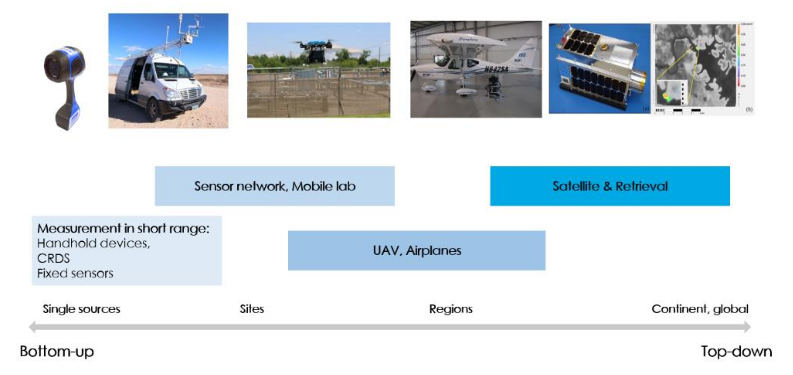
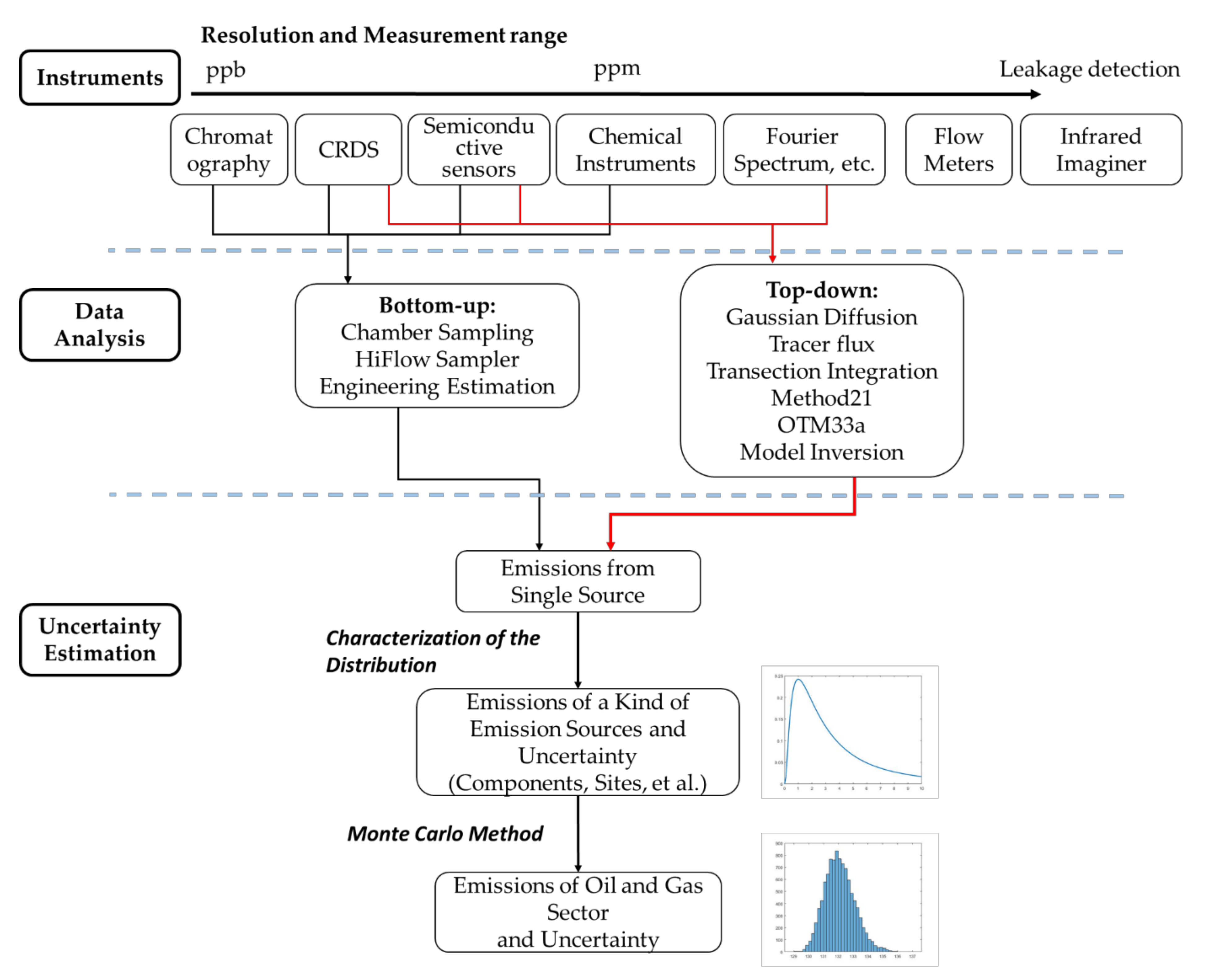
Publisher’s Note: MDPI stays neutral with regard to jurisdictional claims in published maps and institutional affiliations. |
© 2021 by the authors. Licensee MDPI, Basel, Switzerland. This article is an open access article distributed under the terms and conditions of the Creative Commons Attribution (CC BY) license (https://creativecommons.org/licenses/by/4.0/).