Mapping the Energy Flows and GHG Emissions of a Medium-Size City: The Case of Valladolid (Spain)

Abstract

Valladolid (Spain) is a medium-size city (~300,000 inhabitants) that established a greenhouse (GHG) emissions reduction target in 2011 of 20% from 2010–2020. However, tracking the evolution of GHG in medium-size cities is challenging due to the general lack of compulsory data collection at this scale and issues with boundaries when attempting alternative estimates. Here, we propose and apply a novel method to estimate the evolution of GHG emissions due to energy consumption for the period of 2010–2019 in Valladolid, combining top-down and bottom-up data following a physical energy flows approach. The energy consumption of the city is estimated by main sectors and types of energies. The results show that, throughout the past decade, both total energy consumption and its sector end-use share did not significantly change: final energy consumption remained at around 24 MWh (86.5 GJ) per capita and was still highly dependent on fossil fuels, especially natural gas and oil products (over 70% of total energy supply). The GHG reduction by 2019 was ~11% with relation to 2010 and, thus, had not reached the set objective; in per capita terms, the GHG reduction was lower (~6%) due to population loss during the period. The trend, however, has not been monotone and has instead followed a U-shape strongly correlated with the economic crisis and subsequent recovery, suggesting that transition policies have had, at most, a modest effect on the overall results. The analysis shows, first of all, the limitations of statistical sources at a local level, both for energy and mobility, which do not allow more accurate results in identifying the main energy consumers to be reached; and, secondly, the need for strong decarbonization measures which have to be set urgently at all the relevant institutional levels. Reaching GHG neutrality in the city by 2050 requires reducing the GHG emissions by ~13%/year, which is ~20 times faster than for the 2010–2019 average of 0.6%/year.

1. Introduction

The current global sustainability crisis has multiple facets, as the planetary boundaries framework shows: climate change, biosphere integrity, biogeochemical flows, and a land–system change which can exceed the boundaries of each “safe operating space for humanity” proposed in the literature [1]. Together, the acceleration of environmental degradation processes can threaten the continuity of human societies, especially due to climate change [1,2,3]. There are tipping points in climate change that can have large-scale impacts on societies and ecosystems [4]. There is robust scientific evidence that ongoing climate change is associated with the human emissions of greenhouse gases (GHG) [5], especially due to the consumption and way of life of the richest people [6,7]. The majority of GHG emissions are due to the burning of fossil fuels and industrial processes (65%), followed by methane emissions (16%), deforestation and changes in land use (11%), emissions of nitrous oxides (6%), and fluorinated gases (2%) (data from 2010 [2]).

Over the past decade (2010–2020), mitigation (reducing GHG emissions) and adaptation (adapting life to the expected future climate) policies have evolved. The decade began with the reference to the Copenhagen Agreement of 2009 (COP15), which maintained the agreements of 1997 (Kyoto Protocol) regarding the efforts of each country to reduce their emissions, but this time with the information provided by the 4th IPCC Assessment Report [8]. In 2015, after the 5th IPCC Assessment Report [2], the Paris Agreement (COP21) was reached, which proposed a review of the agreements previously adopted and set the objectives to contain the global temperature rise below 2 °C, although the objectives that each country has assumed may not be enough [9].

Many of the mitigation and adaptation strategies adopted in the last decade are designed for the local level [10,11]. In Europe, the institutions have been deeply concerned to promote this type of policy, so there are numerous experiences [12]. In addition, consortia of cities have been set up to promote this type of action (i.e., https://www.c40.org/ (accessed on 29 June 2021) for larger cities or https://energy-cities.eu/ (accessed on 29 June 2021)). Among them, we can highlight the Covenant of Mayors (CoM), which came into existence in 2008 at the initiative of the European Commission and currently brings together more than 10,000 localities [13]. According to the evidence, this initiative has been far-reaching and has helped to implement action plans to mitigate emissions at the local level [14].

There are multiple methodologies and approaches to analyze the energy consumption of a city [15]. We take one physical approach for the final energy consumption user, as in the reference work for Melbourne [16]. This approach has recently been used for two larger Spanish cities: Madrid [17], in which an energy balance is carried out with top-down data sources, and Valencia [18], in which a combination of top-down and bottom-up methodologies are used to solve the lack of data. There are other methodologies to describe the final energy consumption, adopting only a bottom-up approach [19,20,21,22]. In addition, there is a wide range of methodologies linked to the urban metabolism discipline [23,24], which is combined with a social activity analysis [25,26] or other sustainability indicators [27,28,29]. On the other hand, there is also a consumption approach that has similarities with the consumption area based on carbon footprint methodologies [30,31,32]. That kind of analysis usually takes economic input–output data instead of energy physical flows [33,34].

The main objective of this analysis is to identify the main local energy flows and the resulting GHG emissions by sector and type of energy for the case of the medium-size city of Valladolid (Spain). Given that data at this institutional level is typically scarce and that local institutions have difficulties to make their own estimations, we developed a novel methodology which could easily be extended to other similar cases.

Two methodological issues are discussed. The first is to find suitable data sources for the scope of the study. The second is to adopt the perspective and methodology that best allow us to achieve the main objective.

In identifying the main energy-consuming activities in a medium-size city, in our case, we dealt with two main issues that have required the development of novel methodological solutions:

• The lack of detailed and precise statistical data sources;
• The lack of bottom-up methodologies in the literature for the available data.

The study focuses on final energy consumption flows and their purposes over the last decade. Identifying energy consumption purposes tells us which activities consume energy in the city. Knowing which activities consume energy and quantifying this consumption makes it possible to identify the agents that can intervene in a more decisive way in the energy transition. Identifying where the energy is consumed allows us to identify who can modify the consumption patterns. In addition, as the final stage, the characterization of energy consumption flows allows the GHG emissions to be estimated by applying carbon intensity factors.

Data limitations prevent us from incorporating the embodied energy in manufactured goods and services, which have been shown to be relevant for rich economies [35] to the analysis, but this issue is included in the discussion section together with some discussion of hypothetical ranges.

In our case study, Valladolid is a city that signed the Covenant of Mayors in 2011, endowing itself with a strategy—the Sustainable Energy Action Plan (SEAP)—for the mitigation of emissions for 2020 with a reduction objective of 20% [36]. Valladolid’s SEAP template, completed biannually by the local energy agency (AEMVA), provides some information about the final energy consumption of the end users in the city (thus, we took this as an information source), but without a sufficient level of detail. That is why we explain the different data sources to characterize the final energy flow in the city. This approach is relevant due to the characteristics of the city of Valladolid (a medium-size city). We adopt this definition based on the fact that there is a city with around 300,000 inhabitants in its local administrative unit (LAU) and a functional urban area surrounding it (definitions from [37]). The OECD [38] defines it as a medium-sized urban area (between 200,000 and 500,000 inhabitants). In Europe (the EU-27 and the UK), 34% of the urban population resides in urban areas of this type, which account for 17% of the existing urban areas, while in Spain, 35% of the population reside in such areas and account for 34% of the urban areas [37]. In many cases, as in our case study, these urban areas are made up of a large city and the rest of the area is made up of smaller municipalities that rarely reach the category of city (minimum 50,000 inhabitants in the LAU).

The manuscript is organized as follows: Section 2 describes the materials and methods, while Section 3 provides the results, which are discussed in Section 4. Finally, Section 5 gives some conclusions.

2. Materials and Methods

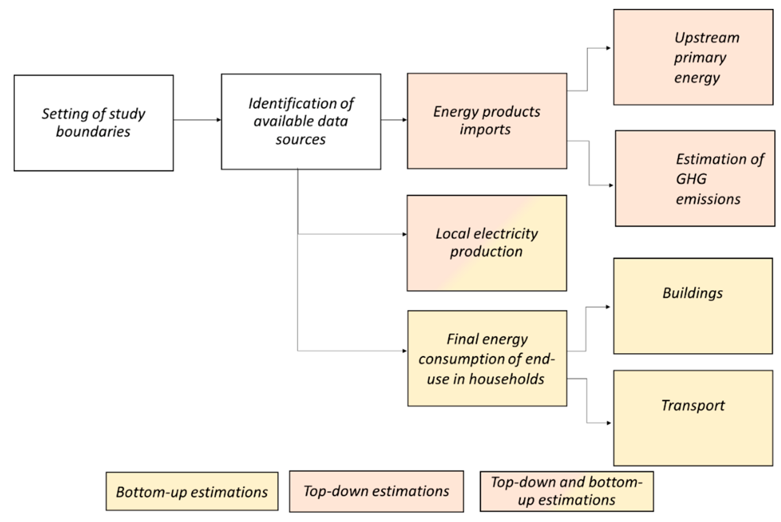
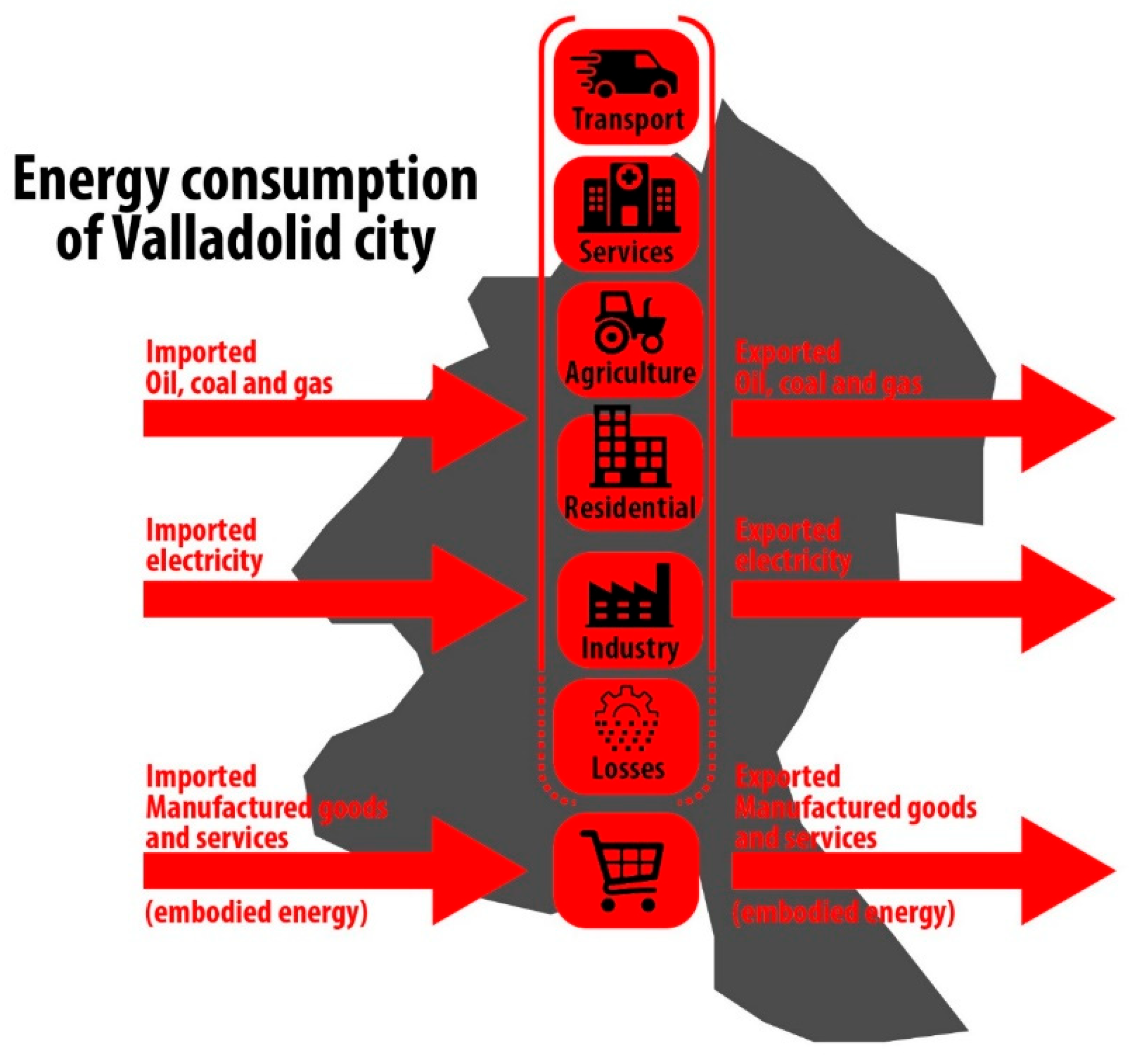
2.1. Overview

In this methodology section, the process is presented in the same order followed to obtain the results shown for Valladolid (Figure 1). The recommendations of the United Nations Statistics Division [39] are followed throughout the entire analysis, especially the one affecting the energy flows and energy product definitions.

After characterizing the case study in Section 2.2, the process begins by defining the temporal, territorial, and sectorial boundaries of the study and the energy flows considered (Section 2.3). Having defined the boundaries of the analysis, the different statistical sources available on consumed energy are analyzed, selecting those that allow a greater definition (Section 2.4). Then, the data sources on produced and self-consumed energy in the reference territory are analyzed. Finally, general statistical information concerning the municipality (population, income, employment, surface…) is collected as auxiliary data.

For this task, it is necessary to overcome the absence of any territorial statistical systems with enough level of detail and with all the sectorial breakdown recommended in [39]. This is due to the lower capacities of the medium-size municipalities to manage their statistical information, unlike the larger municipalities.

Based on the available data, the final energy consumption (equivalent to the energy products imports) is estimated for each sector (Section 2.5) from a top-down perspective. To do this, a series of assumptions that supplement the limitations of the data sources are made. This estimation is performed by adopting an upstream perspective, accounting for the final energy flows that “enter” as imports into the study boundaries, so the energy imports can be estimated (Figure 2), also on the understanding that the city does not export final energy flows. When data are not provided on the local level, we take the larger territorial units (Spanish provincial level—NUTS level 3 [37]) and apply different downscaling factors, depending on the sector and energy source. Downscaling is a usual way to perform estimations at local level when there are not enough local information sources [21,28], but there is no systematic method for this approach. We adopt this perspective as it seems to be the closest to actually knowing the energy flows that are transformed into useful energy in the area of study, thus allowing us to estimate the energy product imports that are required. The main methodological contribution of this work is the downscaling factor choices, a systematic approach which can be useful for the estimation of energy flows and GHG of other medium-size cities. The calculation of the electric energy produced and self-consumed in the scope of the study is also incorporated due to the transformation and production of primary products (Section 2.5.2). This estimation allows us to understand the importance of the self-produced energy, despite the fact that it is not an energy flow.

Taking the final energy data, the upstream primary energy linked to the energy imports is calculated, so as to obtain the quantification and characterization of the total energy supply (TES) (Section 2.5.3). Finally, the GHG emissions produced due to the final energy consumption are also calculated with the help of sectorial carbon intensity factors (Section 2.5.4).

After obtaining the general perspective of the energy flows consumed and their sectorial breakdown from a top-down perspective, we estimated the energy directly consumed by the households following a bottom-up approach (Section 2.6). The purpose of this estimation is to identify the energy demand due to the households in order to prevent an eventual overestimation from the top-down perspective to this sector. To do so, we provided two calculations with a bottom-up methodology to obtain, firstly, the energy consumed in the residential buildings and, secondly, the energy consumed by the mobility of the resident population. For the first one, there are many models [40], and there is abundant official data at our study case level concerning this subject (cadastral data [41]), which allows acceptable results to be obtained. On the other hand, for transport, there are far fewer models and information sources. Although the transport consumption calculation could be based on the existing vehicle fleet (on which there is abundant information), there are important differences between this fleet and its actual use [42]. That is why we opted for sources that describe personal mobility to estimate energy consumption, which is another novel method developed for this work. In this regard, we found two types of sources: urban mobility surveys and interurban mobility surveys or databases. It is not usual for these data sources to directly collect energy consumption estimates; thus, it is necessary to make estimates, as we did in this case.

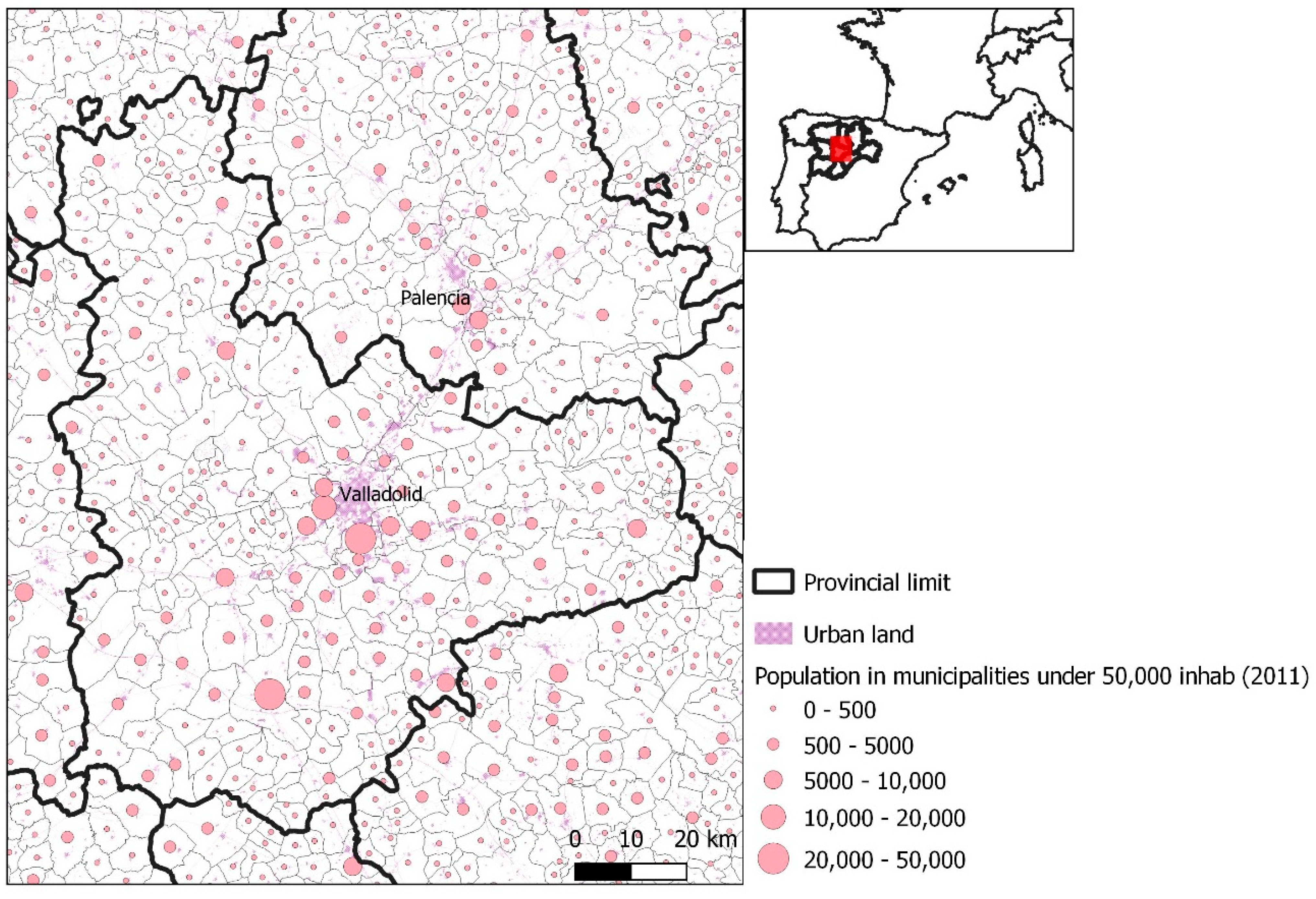
2.2. Description of the Case Study

The city of Valladolid has a municipal area of 197 km², of which 75% is rural land, and has around 300,000 inhabitants. Furthermore, the rest of the province (~500,000 inhabitants), although it is mostly rural, has several large municipalities (over 20,000 inhabitants) [43]. Some of these municipalities are located on the periphery of the city of Valladolid (Figure 3), forming a functional urban area. Laguna de Duero, south of Valladolid, has been a municipality of more than 20,000 inhabitants for decades. Arroyo de la Encomienda has also become a large municipality in the last decade, which has grown by 30% to reach 20,000 inhabitants. The urban area that surrounds Valladolid is home to about 20% of the population of the province that does not reside in Valladolid. In total, the functional urban area (Valladolid and periphery) accounts for almost 80% of the population of the province with ~400,000 inhabitants [44].

Valladolid has a relevant position as, for decades, it has been the biggest city in the north-west regions of Spain (Castile-and-León, Asturias, Galicia) [44]. The city has large industrial zones due to the presence for over half a century of an important automotive construction sector, today represented by Renault and Iveco plants. Later, other important industrial plants, such as Michelin (petro-chemical sector) or Entrepinares (food sector), consolidated the industrial profile of the city [45]. In addition, it is an important transport node, both for passengers and freight transport. The city has a large rail infrastructure (with high-speed trains directly linking the city with Madrid), and the E-80 Trans-European Motorway, which links Portugal with France, passes by. The airport serving Valladolid is located next to a nearby village, Villanubla (less than 20 km).

2.3. Setting of Study Boundaries

First of all, the study is temporally and geographically limited. A ten-year time range is chosen with annual data as a sample. In the case analyzed, considering data availability, the decade 2010–2019 was chosen. Secondly, the approach is area-based. This second delimitation implies some complications with diffuse energy uses, among which transport stands out, due to the relationship with the rest of the functional urban area and also to the importance of being a transport transit hub. In order to identify the transport energy consumption, the interurban mobility is taken as inner energy consumption only for the road modes, which can refuel in the city area. Therefore, it is assumed that the energy imports to the reference area are the main indicators of the final consumed energy; this is also true for the transport sector. In addition, it is the main data source to estimate the GHG emissions due to local activities.

It is important to point out that, in our analysis, we focus solely on GHG emissions from energy consumption, which are globally the main source of GHG, followed by agriculture, forestry, and other land use [2]. Note that the latter generally occurs in rural areas; however, in the case of Valladolid, this means two bovine farms which host over 4000 heads of cattle must be excluded. On the other hand, the grid electricity GHG emissions are not produced in the city area. Nevertheless, we consider them as emissions due to the energy consumption. This is an important aspect that differentiates our work from city-level carbon accountability [31].

Regarding the energy flows considered, the final energy consumption is taken as the energy consumed in the city, so the end-use transformations are excluded (those energy transformations that do not become an energy product). The main energy flow which affects our reference territory is the energy imports, followed by such “internal flows” as transformation or production. Other flows that can be analyzed, such as energy exports or stock, are negligible in this case. The energy embodied in imported/exported goods and services is also excluded from the analysis.

The upstream primary energy supply represents the TES (defined in [39]). These energy flows include the primary commodities before they become the energy products that arrive at the city boundaries after the transformation, stock, and transport processes, which occur outside the city boundaries.

The “internal flows” comprise the transformations and production of energy products that occurs in local energy industries; which, in this case, are electricity, combined heat and power (CHP), and heat plants. This analysis only reports the electricity production in order to compare it with the energy product imports, specifically with the imported electricity. Therefore, heat products are excluded from the analysis. Furthermore, the CHP plants linked with different industrial processes, such as auto-producers, are set aside. Only the biggest one, linked to the Michelin plant, is taken into account, because it can sell an important amount of electricity to the grid. Two CHP plants linked to public services plants (sewage and waste treatment) are also reported, as they run on locally produced biogas.

The heat energy production of these plants is not included in the analysis for two reasons. The first is the lack of sufficient accurate data for this, due to the limitations of the heat accountability, in both the CHP plants and the solar heat installations. The second is that the heat energy produced is usually end-use energy, which is excluded from the analysis as it is not an energy product (with the sole exception of the heat production from the district heating installed in 2014 [46]). Therefore, we assume that the loss of information associated with not reporting the production of heat energy is not very relevant at the municipality level, as we concentrate on the energy products that are imported by these plants (natural gas for CHP and biomass for the district heating plant), so its estimation is left for future work.

2.4. Identification of Available Data Sources

Official statistical data sources were given priority, but when these did not provide sufficiently precise data, we complemented them with other sources or our own estimates. General data on the municipality (population, employment by sectors, surface area, agricultural area) were obtained from institutional statistical services [43,47]. The data sources on energy consumption and bottom-up modeling are presented in

Table 1. Available data sources per sector and type of energy.

Sector	Final Energy Consumption	Energy Production	Temporal Range	Territorial Level	Source	Observations
All	Electricity	-	2010–2016	NUTS3	[48]	Sectorial breakdown until 2016, total data until 2019
All	LPG	-	2010–2016	NUTS3	[48]	Sectorial breakdown until 2016, total data until 2019
All	Natural Gas	-	2010–2016	NUTS3	[48]	Sectorial breakdown until 2016, total data until 2019
Transport, Agriculture	Oil products	-	2010–2019	NUTS3	[49]	We assume that each type of oil product is for one use (Gasoline and Diesel oil—type A for transport, Diesel oil—type B for agricultural uses and Diesel oil—type C for heating buildings)
All	All	-	2010–2019	City	[50]	Just for even years. Exclude big industries. Underestimate electrical consumption.
Public sector	All	-	2010–2019	City	[50,51]	Regional administration offer detailed data since 2017
University	All	-	2010–2019	City	Directly provided by Universidad de Valladolid
CHP plant (Energyworks vitvall)	Natural gas	All	2010–2019	City	[52,53]
CHP plant (sewage)	-	All	2018–2019	City	[54]
CHP plant (waste treatment)	-	All	2015–2018	City	[55]
Photovoltaic solar plants	-	Electricity	2010–2019	City	[56]
Buildings surface	None	-	2010–2019	City	[41]	Surface of residential buildings for each year
Urban mobility	None	-	2015	City	[57]
Interurban mobility	None	-	2017	NUTS1	[58]

. The primary data are also available in the Supplementary Materials.

2.5. Estimation of Energy Flows and GHG Emissions by Sector and Type of Energy

2.5.1. Estimation of Energy Products Imports

As indicated, different assumptions are made for each energy source and sector. Most of the energy product imports are calculated through downscaling from the provincial data (NUTS3 level) and later cross-checked with the city council inventories [50] to confirm the quality of the estimation. They report reliable data just for some years (even years from 2012) and energy sources (natural gas for some sectors, LPG, biomass). The downscaling method is a better approach for the energy products whose consumption occurs in the diffuse sectors.

The different downscaling factors applied are chosen under the following criteria:

• They are an accurate indicator of sector size;
• They are common data, easy to obtain even in small-size cities;
• They are complete time series.

When possible, data are taken directly from the city council data. This is the case of the biomass data, derived from AVEBOIM (a Spanish biomass sectorial association), or the oil products consumed by the public sector provided by official sources [50,51]. For those years without enough data, extrapolations are carried out, maintaining the sectorial share. The method applied in each case is shown in

Table 2. Estimation method for each energy product and sector. For “Direct source” see Table 1.

Energy Product	Sectorial End-Use	Estimation Method	Downscaling Factor	Observations
Biomass	Agriculture	Direct source	-
	Commerce and public services	Direct source	-
	Household	Direct source	-
	Industries	Direct source	-
	Transport	Downscaling	% city’s population over provincial	The percent of biofuel provided by the distributor is applied [49]
Electricity	Agriculture	Downscaling	% agricultural surface over provincial
	Commerce and public services	Downscaling	% city’s services employment over provincial
	Household	Downscaling	% city’s population over provincial
	Industries	Downscaling	% city’s industrial employment over provincial
	Transport	-	-
Natural gas	Agriculture	-	-
	Commerce and public services	Downscaling	% city’s services employment over provincial
	Household	Downscaling	% city’s population over provincial
	Industries	Downscaling	% city’s industrial employment over provincial	We assume that the highest pressure and consumption installations are the industrial.
	Transport	-	-
Oil Products	Agriculture	Downscaling	% agricultural surface over provincial
	Commerce and public services	Direct source	-	The oil products consumption in this sector is a small fraction of heating oil reported by [50].
	Household	Downscaling	% city’s population over provincial	The LPG consumption is weighed by a factor of 0.5 due to the lack of isolated buildings in city.
	Industries	Direct source	-	The oil products consumption in this sector is a small fraction of heating oil reported by [50].
	Transport	Downscaling	% city’s population over provincial	The LPG consumption is added, mainly due to the urban public transport [50].

and the different downscaling factors in

Table 3. Population and employment indicators used as downscaling factors.

Data	Units	Source	2010	2011	2012	2013	2014	2015	2016	2017	2018	2019
City population	People	[43]	315,522	313,437	311,501	309,714	306,830	303,905	301,876	299,715	298,866	298,412
% city’s population over provincial	%		59.13%	58.60%	58.30%	58.19%	57.98%	57.74%	57.65%	57.51%	57.49%	57.44%
City employment	People	[47]	118,100	116,938	114,503	112,177	114,390	118,161	120,199	124,135	128,274	130,842
City industrial employment	People		17,638	17,825	17,079	16,569	16,854	17,991	19,204	19,586	19,768	20,363
% city’s industrial employment over provincial	%		62.25%	62.61%	62.85%	62.80%	62.67%	62.75%	63.46%	63.06%	62.68%	62.57%
City services employment	People		91,382	91,281	91,052	90,293	92,119	94,690	95,541	98,794	102,289	104,099
% city’s services employment over provincial	%		78.07%	77.95%	77.41%	77.55%	78.20%	78.24%	77.62%	77.37%	77.25%	77.05%
% agricultural surface over provincial	%	[43]	1.70%	1.70%	1.70%	1.70%	1.70%	1.70%	1.70%	1.70%	1.70%	1.70%

.

The downscaling method implies accepting the assumption of proportionality between the variables energy consumption and the factor chosen: population, agricultural surface or employment. There are increasing works in the literature about urban scaling that show the existence of these kind of relations in many cities [59,60,61]. However, in this case, the comparison is between the urban and rural zones that make up the territorial unit and not between different urban zones. Even in this case, these scaling laws appear [62]. Despite the scarcity of evidence for the relationship between population and energy consumption in transport uses (shown in the literature), it is enough to neglect other factors.

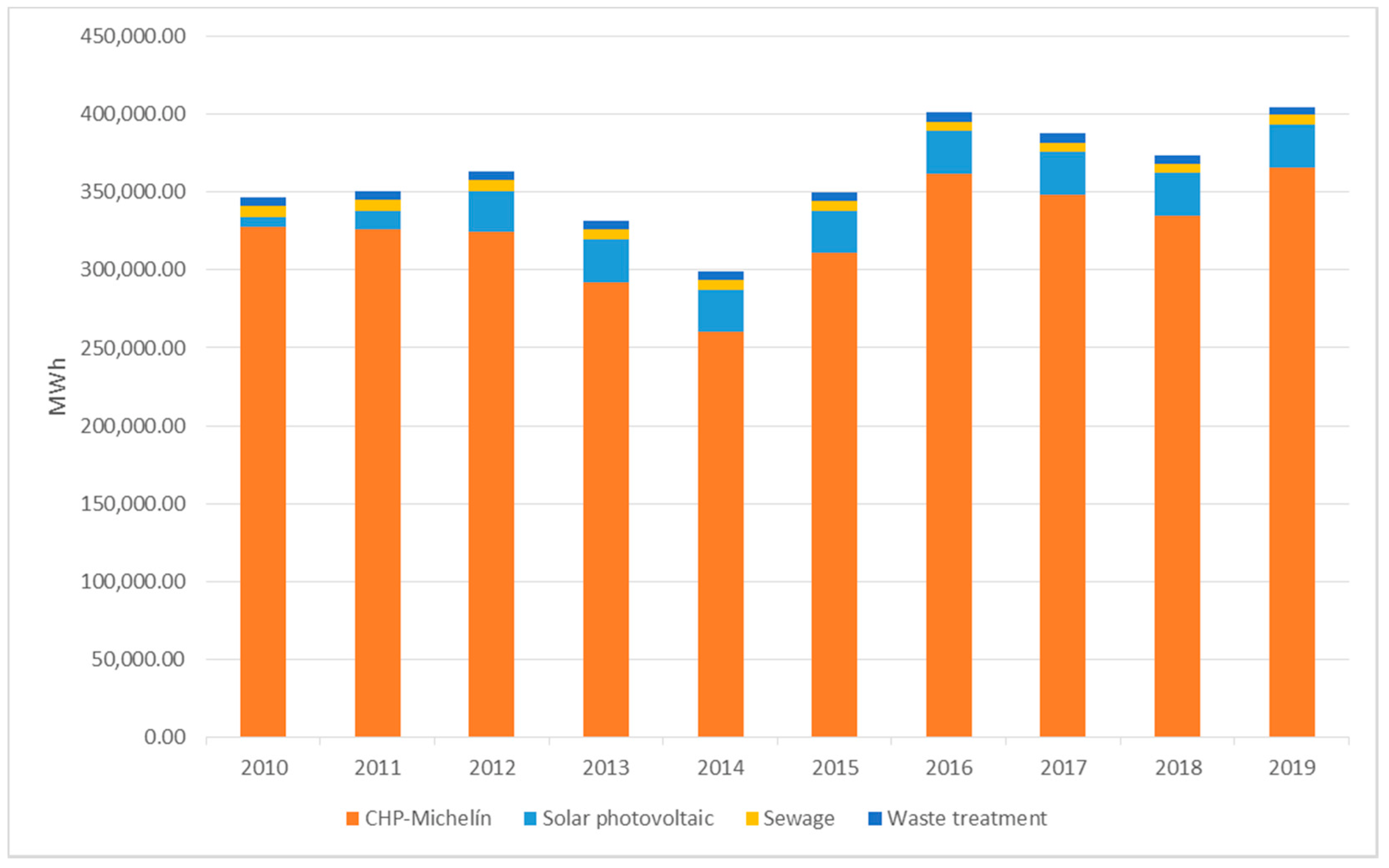
2.5.2. Electricity Local Production

There are two types of significant electricity producers in the municipality: centralized electricity production plants (in our case, centralized plants based on natural gas or biogas) and distributed solar production.

To estimate the consumption for the first type (centralized plants), we used two methods of estimation, one with a top-down and the other with a bottom-up perspective, as detailed below.

• For the Michelin power station (Energyworks VitVall PlantValladolid, Spain), due to the fact that it is the only major consumer in the town, its electricity production could be estimated with its performance characteristics (0.39 MWh of electrical output for each 1 MWh of natural gas supply [53]) and gas consumption data from the distribution company. We could test that data with the emissions reported in the UE-ETS database [53].
• For the plants associated with the treatment of sewage sludge (water treatment plant) and solid waste, we had reports with the electrical energy production data for some years of the series [54,55]. We estimated the rest of the series assuming that production is proportional to the population served by each plant (the water treatment plant in the town and the solid waste treatment plant in the province).

A bottom-up perspective is adopted to estimate the energy produced through distributed solar installations. We started from the inventories of installations [56] and applied average production factors for photovoltaic solar energy, i.e., 1580 MWh-year/MW-installed [63].

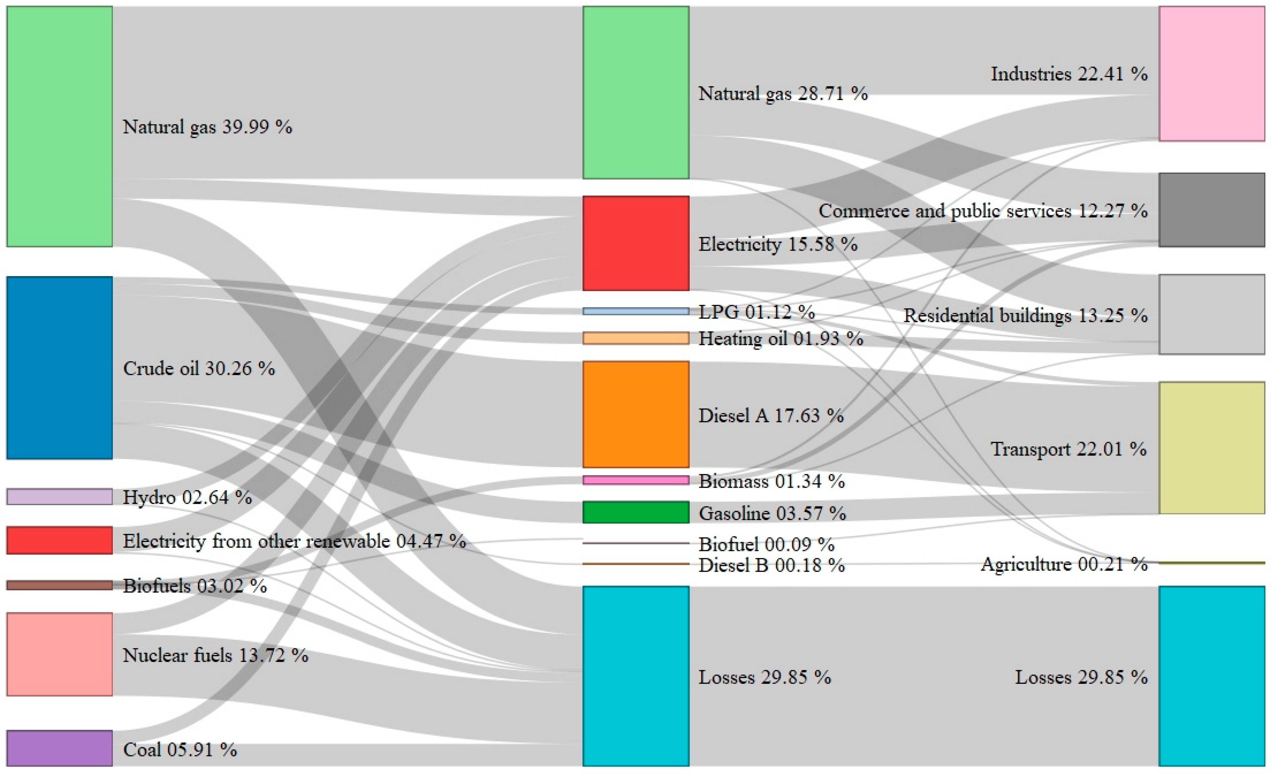
2.5.3. Upstream Primary Energy

We calculated the upstream primary energy imports from the data collected as energy product imports (Section 2.5). Based on these data, we applied different conversion factors provided by [64] (see

Table 4. Upstream primary energy conversion coefficients. Source [64].

Energy Product	Primary Energy Product	Conversion Coefficient [MWh p/MWh f]
Gasoline	Crude oil	1.24
Diesel A	Crude oil	1.26
Diesel B	Crude oil	1.26
Biofuel	Liquid biofuel	2.11
Liquid gas	Crude oil	1.12
Biomass	Solid biomass	1.36
Heating Oil	Crude oil	1.26
Natural gas	Natural gas	1.15
Electricity	Hydropower	1.07
Electricity	Nuclear fuel	3.9
Electricity	Hard coal	2.69
Electricity	Crude oil	2.76
Electricity	Natural gas	2.15
Electricity	Electricity from other renewable	1.07

). For the electricity factor, it was assumed that the energy is distributed with a low voltage. For the rest of the products, the most representative categories were selected. It was assumed that, throughout the decade studied, there were no relevant technological changes that led to modifications in the conversion factors from primary energy to final energy, so they were taken as constants.

It should be considered that the energy mix of electrical energy changes every year, so the percentage of energy consumed by each primary energy source that participates in the grid electrical was weighted by the annual energy mix of the electrical system, offered by REE [65].

The addition of these imports offers the TES of the city.

2.5.4. Estimation of GHG Emissions

Analogous to the calculation of the upstream primary energy imports, GHG emissions due to the final energy consumption were computed from the energy product imports and the corresponding emission factors were applied from [64]. These factors included the whole life-cycle of each energy product. The same assumptions were made as for the primary energy estimations. In the same way as for the previous estimate, we assumed these factors to be constant, except for the case of electric energy. Figure 4 shows how the emissions related to electricity consumption in Spain underwent significant variations during the study period, related to the variability of the hydroelectricity due to the Mediterranean weather. However, the drop in emissions at the end of the decade is related to a reduction in the carbon intensity of the electrical generation mix, which is mainly due to the policies that led to switching off coal power plants [66]. The results for an uncertainty analysis, to account for the estimated higher GHG emissions related to CH₄ leakages, are presented in the Section 3.

2.6. Final Energy Consumption of End-Use in Households

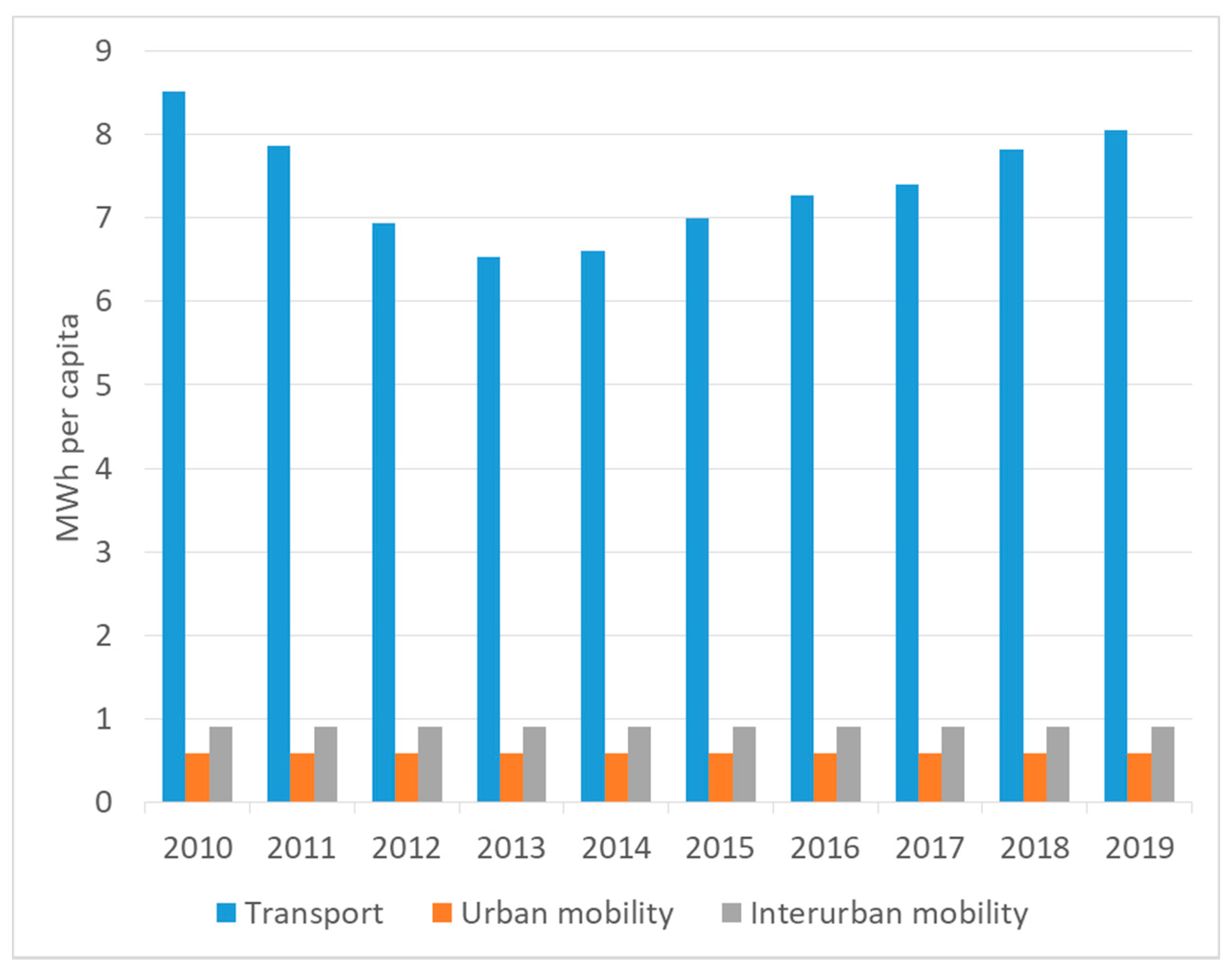
A bottom-up estimation of household energy demand is also made in this work to complement the top-down estimate. If the bottom-up perspective finds differences with the top-down perspective, it means that there is an overestimation or underestimation of the sector’s consumption, or that there is some consumption behavior hidden from the bottom-up approach.

2.6.1. Transport

Energy consumption due to the personal mobility of the population makes it necessary to distinguish between urban mobility (passenger trips between zones in the city) and interurban mobility (passenger trips between the city and other places).

The share of energy consumption corresponding to urban mobility was calculated based on the mobility data collected in the 2015 mobility survey [57]. The methodology we adopted is similar to the one used in [21], which used an estimation of the transport energy consumption based on commuter mobility. In our case, the survey offers several panels with the total number of trips between zones for each means of transport (pedestrian, private vehicle, public transport, others). By calculating the distance between each zone, it was possible to obtain the transport production data that are carried out daily in passenger-km units. The distance ($\overline{d_{ij}}$ in Equation (1)) measured is the radius of gyration used in the mobility patterns literature [67]. The internal trips of each zone were assumed to be 0.5 km. This hypothesis was adopted as these trips are mostly pedestrian and are, therefore, short. In addition, the median size of these zones is 1.32 km² and the biggest are the least populated. In any case, although they are important within the total distribution, as they are mostly by pedestrian mode, they affect the local energy consumption estimation relatively little.

Once the transport production values were obtained, we estimated the energy consumption linked to each mode, applying the factors shown in

Table 5. Urban mobility energy consumption calculation.

Data	Year Production [pass-km]	Num of Passengers [pass-km/veh-km]	Fuel Consumption [l/veh-km]	Fuel Density [kg/l]	Fuel Energy Intensity [MWh/ton]	Transport Energy Intensity [MWh/veh-km]	Mobility Energy Consumption [MWh]
Source	Own estimation			[68]		Own estimation
Pedestrian	157,416,492	1.00	0.00	-	-	-	-
Other	28,857,311	1.00	0.00	-	-	-	-
Private vehicle	189,573,302	1.50	0.10	0.75	12.31	0.00	116,174
Public transport	93,433,879	7.50	0.50	0.83	11.94	0.00	61,902
Total	283,007,181	-	-	-	-	-	178,076

using Equations (1)–(3).

$$Transportproductio{n}_{ij}\left[\mathrm{pass}\text{-}\mathrm{km}\right]\approx \overline{d_{ij}}\left[\mathrm{km}\right]·trip{s}_{ij}\left[\mathrm{pass}\right]$$

(1)

$$\begin{array}{c}Mobilityenergyconsumption\left[\mathrm{MWh}\right]\hfill \\ =\sum Transportproductio{n}_{ij}\left[\mathrm{pass}\text{-}\mathrm{km}\right]\hfill \\ ·transportenergyintensity[\mathrm{MWh}/\mathrm{pass}\text{-}\mathrm{km}]\hfill \end{array}$$

(2)

$$\begin{array}{c}Transportenergyintensity[\mathrm{MWh}/\mathrm{pass}\text{-}\mathrm{km}]\hfill \\ =numofpassengers[\mathrm{pas}\text{-}\mathrm{km}/\mathrm{veh}\text{-}\mathrm{km}]·fuelconsumption[\mathrm{l}/\mathrm{veh}\text{-}\mathrm{km}]\hfill \\ ·fuelenergydensity[\mathrm{MWh}/\mathrm{l}]\hfill \end{array}$$

(3)

For the energy estimation due to external mobility, information was extracted from the mobility data from geolocated data provided by official sources [58]. We then assumed that the energy used in the total number of trips of the resident population was considered as local consumption. This hypothesis cannot be applied for certain modes of transport: there are no airports or ports in the municipality of Valladolid, so energy is not consumed locally for trips by plane or boat. The electrical consumption due to trains is distributed along the railway, so we do not take that into account as relevant local energy consumption. However, people do refuel many of the vehicles that pass through the city, either as origin or destination. A simplifying criterion was assumed, where the energy consumption of all the resident trips by road transport modes are imputed to the local energy consumption.

Starting from the indicated data source, there is a series of transport production in passenger-km units classified by the purpose for each journey (home, work, frequent, spontaneous). We exclusively took trips to Valladolid from home or work, or from Valladolid to home or work, assuming that these trips will be the ones that reflect those of the resident population (from any type of origin and to any type of destination).

With these data, a weighting of the different types of days offered by the database was carried out (summer weekday, summer weekend, non-summer weekday, non-summer weekend). In addition, a downscaling factor was used to exclude trips due to the rest of the province’s population. To achieve this, we assumed that the trips of the city population were the proportional part of the population over the province.

With the total mobility produced in passenger-km, Equation (2) was used with the energy intensity for each transport mode, taken from [69], to obtain the energy consumed by this type of mobility, as shown in

Table 6. Interurban mobility energy consumption calculation.

Data	Transport Energy Intensity [MWh/veh-km]	Annual Production [pass-km]	Mobility Energy Consumption [MWh]	Mobility Energy Consumption in City [MWh]
Source	[69]	[58] and own estimation	Own estimation	Own estimation
Train	0.000108	87,869,500	9446	0.00
Plane	0.000092	35,918,430	3304	0.00
Road	0.000323	838,729,485	270,723	270,723

.

2.6.2. Buildings

We start from the data of the set of existing residential buildings in the municipality. With these data, obtained from the Land Registry [41], it is possible to obtain the total built surface existing in each year of the period studied.

Assuming that the main energy consumption of Spanish homes is destined for air conditioning (mainly heating), we first estimated how much this consumption represents for the residential area each year. To do this, we took the energy factor consumed for heating, cooling, and hot water as constant. We took this factor from the energy certification tool for residential buildings. In the case of Valladolid, the factors are (taking the most common kind of housing): 60.6 kWh/m² for heating, 4.5 kWh/m² for cooling, and 13.3 kWh/m² for hot water [70].

For the rest of domestic consumption, it was assumed that it is proportional to the heating consumption of the average household type [71]. In this way, the average household proportion between heating consumption and other consumption (electrical appliances, kitchen and lighting) was maintained.

Finally, we applied a correction due to the percentage of empty dwellings. We applied a reduction percentage to the total obtained energy consumption equal to the percentage of empty homes. In the case of the province of Valladolid, according to data from the 2011 census, 11.90% of the houses are empty [44].

3. Results

We first describe the temporal evolution of the main outputs resulting from the top-down perspective, and subsequently, taking the data for 2016, we delve into the sectorial breakdown of the different consumptions. We take that year because it represents a middle point, both temporally and within the main tendencies that we analyzed. Finally, the bottom-up estimations are shown in order to describe the specific household energy consumption. The detailed results are included in the Supplementary Materials.

3.1. Temporal and Sectorial Evolution

The evolution of the main indicators can be seen in Figure 5, which shows how the economic indicators (GDP and employment) diverge from the decreasing trend in the population. The TES (primary energy consumption) fell to a minimum in 2014, taking a different pattern from the economic and population indicators. Although energy product imports and its upstream equivalents maintain a very similar evolution, the associated GHG emissions fell in 2019. This is due to the practical elimination of coal from the peninsular grid electricity production.

Regarding the distribution by upstream primary energy, the vast majority of the energy products are from fossil fuels (crude oil and natural gas represent between 70% (2015) and 78% (2010) of primary energy sources). As is shown, biomass consumption multiplied by a factor of 3.45 between 2014 and 2016, due to the district heating installation service of the University buildings [46]. That increase has no clear correspondence with a reduction in other fuels in the whole city overview, despite the large natural gas consumption reduction achieved in the university (a reduction of 76% between 2011 and 2019) and the elimination of the use of heating oil.

Regarding the sectorial final energy consumption,

Table 7. Final energy consumption by year, sector, and energy product. Units: MWh. Source: own estimation.

Energy Product	Sectorial End-Use	2010	2015	2019
Biofuels	TOTAL	12,891	94,282	175,973
	Agriculture	0.00	0.00	0.00
	Commerce and public services	127	45,157	101,284
	Household	0.00	7079	14,210
	Industries	0.00	34,252	48,130
	Transport	12,764	7796	12,350
Electricity	TOTAL	1,544,597	1,523,979	1,541,933
	Agriculture	2064	2513	2223
	Commerce and public services	580,773	458,449	442,615
	Household	498,532	390,337	358,939
	Industries	463,228	672,680	738,156
	Transport	0.00	0.00	0.00
Natural gas	TOTAL	3,044,486	2,462,696	2,863,457
	Agriculture	2878	435	334
	Commerce and public services	584,637	624,929	667,708
	Household	1,012,235	540,073	656,907
	Industries	1,444,735	1,297,260	1,538,508
	Transport	0.00	0.00	0.00
Oil Products	TOTAL	2,953,137	2,371,336	2,592,332
	Agriculture	22,032	17,841	18,229
	Commerce and public services	8539	12,367	17,971
	Household	245,676	219,462	157,350
	Industries	3165	3405	10,643
	Transport	2,673,724	2,118,261	2,388,139
TOTAL	TOTAL	7,555,110	6,452,295	7,173,695

indicates the relevance of the industry in the city. In addition, this consumption went from representing 25% to 34% throughout the decade. On the contrary, residential consumption has significantly and steadily decreased its consumption throughout the decade, falling by 29% at the end of the decade.

In any case, the total final energy consumption in 2019 reached levels very similar to those of 2010 and, in the same way, the TES trend followed a U-shape.

The GHG emissions per capita due to the energy products imported by sector are shown in Figure 5.

The weight of each sector and the evolution along the decade is similar to the final energy consumption obtained. Unlike the final energy evolution, in the last few years of the decade, the GHG emissions went down due to the reduction in the emissions factor of the Spanish grid electric energy (cf. Figure 4).

We must point out that we do not include the fugitive emissions relative to natural gas extraction and transport, which were estimated, for conventional natural gas, at 40.6% higher than those considered in the official databases, and which we also consider here by default [72]. Note that, following that study, the total emissions of conventional natural gas would be 56.1 gCO₂eq/MJ and 0.78 ± 0.45 gCH₄/MJ, which translates into a large GHG increase due to the fact that CH4 has a 100-year GWP of 30 (i.e., 1 g. of CH₄ warms as 30 g. of CO₂ on average during a 100-year period) [2]. This affects the principal natural gas consumers, i.e., residential buildings and industrial processes, as well as the national electricity mix, which would increase the total GHG emissions of the city by between 20% and 25%.

Regarding the evolution of local production, the dynamics are mainly marked by the main CHP, as seen in Figure 6. It also shows an increase in the share of photovoltaic self-consumption throughout the decade. Local photovoltaic energy went from producing the equivalent of 0.3% of the electrical energy consumed in 2010 to 1.8% in 2019.

The sectorial breakdown for 2016 is represented in Figure 7, which shows the importance of natural gas in almost all the sectors (with the exception of transport). There is an important direct consumption of natural gas in industrial uses (51.10% of the final energy consumption of natural gas, 20.99% of the total final energy consumption). In addition, the Diesel A consumption for transport (25.13% of total final energy consumption) reveals the importance of economic activities as energy consumers in the city, while residential buildings consume 18.92% of the final energy share (without accounting for energy transformation losses, which appear on the right-hand side of Figure 7). Taking losses into account implies that residential buildings represent 13.25% of the TES.

Within the main energy consumer sectors, we find the relevant weight of some large consumers. In the industrial consumption, the Michelin CHP stands out with 62% of the gas consumed by the industrial sector and 32% of the total natural gas consumed in the city (2016 data). Similarly, the automotive construction sector accounted for 43% of the electricity consumption of the industrial sector and 20% of the total electricity consumed, which is mainly due to two industrial plants (the Renault España and Iveco España plants).

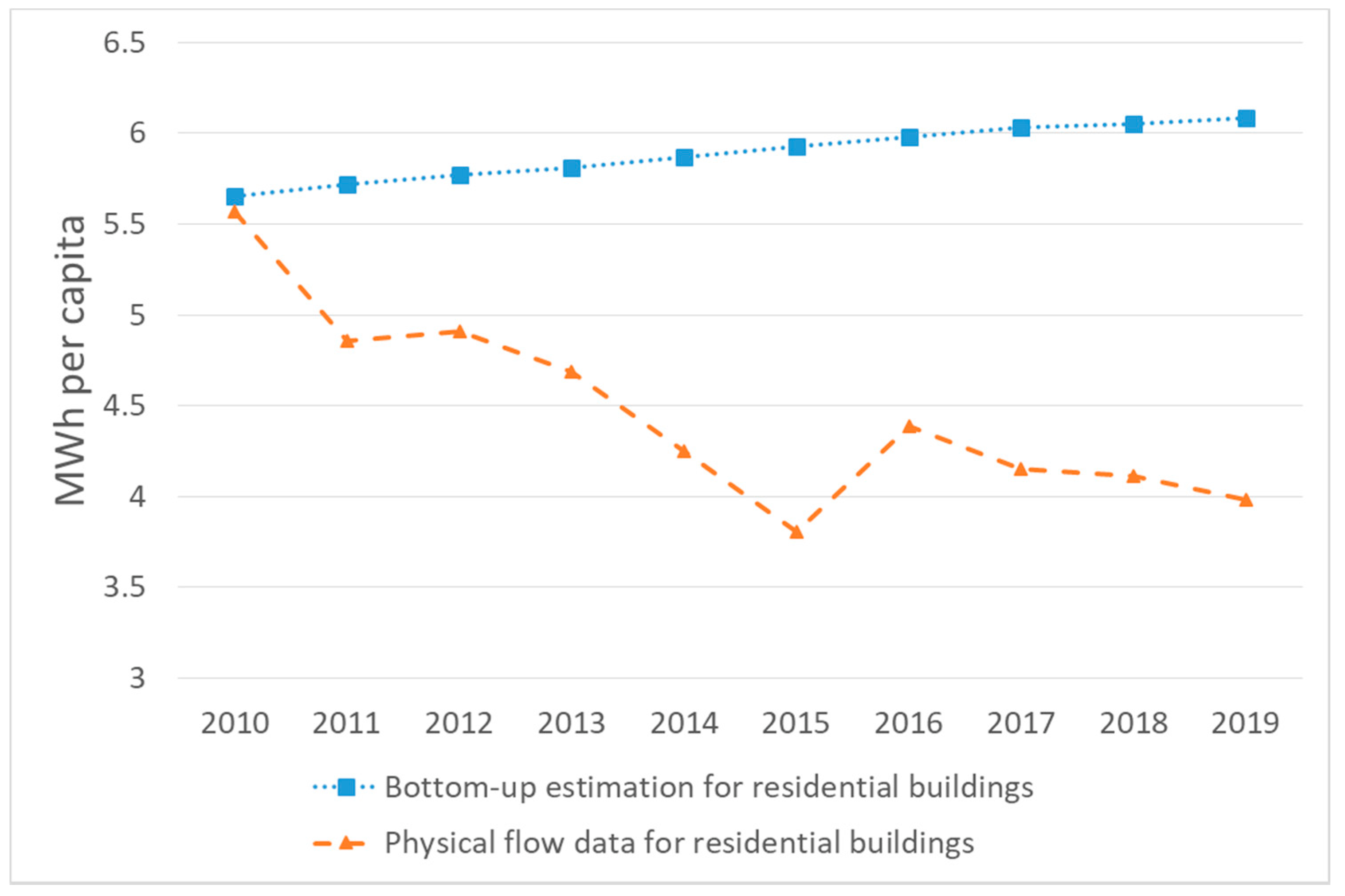
3.2. Final Energy Consumption Estimations Top-down vs. Bottom-up of End-Use in Households

Using the indicated bottom-up estimations, we reached a consumption estimation with two very different results for passenger transport and residential buildings.

Regarding the bottom-up estimated consumption in transport due to urban and interurban mobility, the estimate made only explains between 18% (2010) and 24% (2013) of the fuel consumption attributed to transport in our methodology, which is close to the data collated by the city council [50] (Figure 8). This is despite collecting local consumptions all those consumptions related to road transport of the resident population. In view of this estimate, we can propose two possible explanations: the first is that freight transport is a major energy consumer, and the second is that the top-down fuel estimation used is not accurate enough to obtain local consumption data.

For residential building consumption, the bottom-up estimation shows an almost exact coincidence with the physical flow data for 2010 (Figure 9) and its accuracy then declines throughout the decade. As shown, the difference gets bigger along the decade, reaching a difference of 50% in 2019. This may be due to different factors: increased efficiency in domestic uses, milder temperatures, variations in the composition of homes, an increase in poverty, etc. The bottom-up estimate made is in line with the actual consumption for the year 2010, but the projection thereafter fails, since the bottom-up estimation cannot take into account different factors that can drive important changes in the consumption patterns, especially the social drivers.

4. Discussion

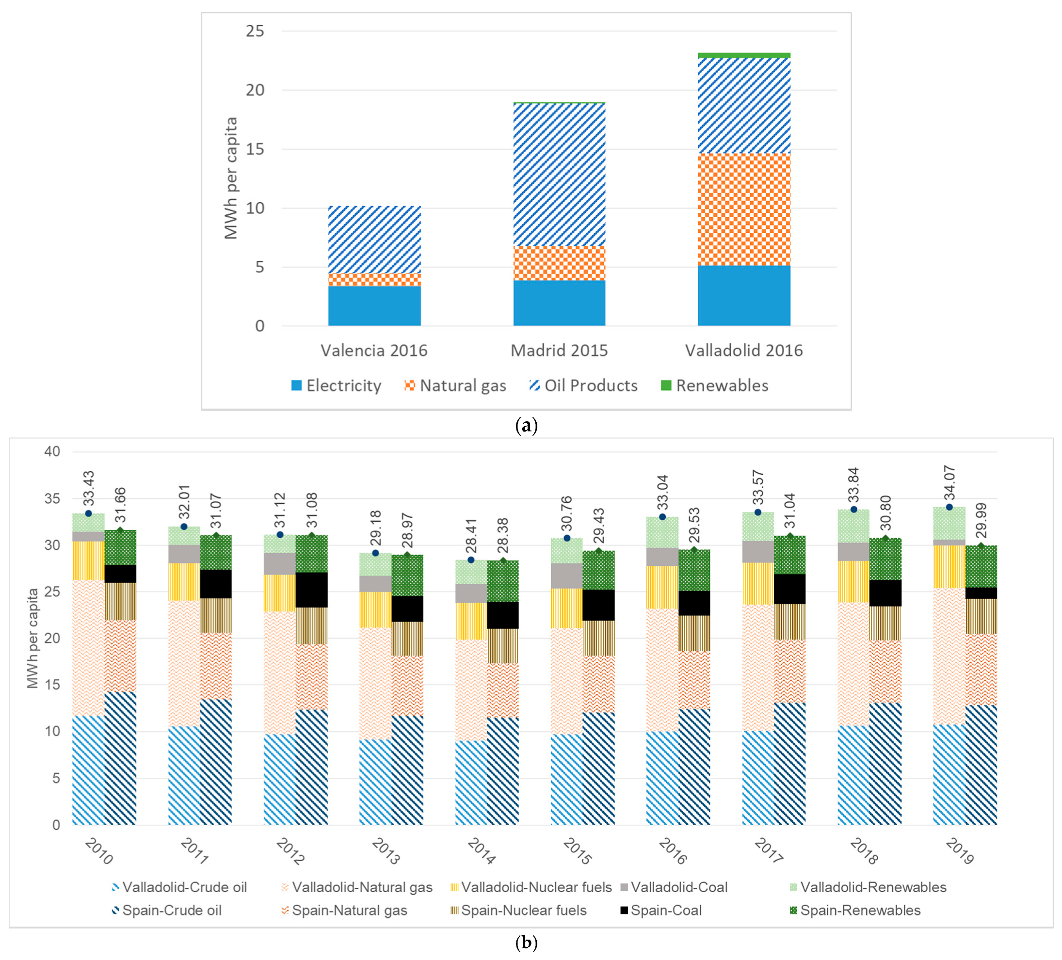
4.1. Comparison with Other Studies and with the Spanish Average

In order to compare the applied methodology and the results obtained with other local realities, we took the energy balances for Madrid [17] and Valencia [18] as references. We took these studies for the geographical proximity and for the similar approach. Concerning the methodology, the Madrid case used only a top-down methodology, while the Valencia case combined it with bottom-up estimations to obtain the sectorial classification. We also compared the results with the average Spanish TES per capita with data from the IEA [73].

Taking the breakdown of energy sources (using the categories of this analysis), we show the comparison between the three cities in Figure 10. An important difference between the three cities is found. Some explanations are offered below.

• The different population size of each city distorts the relative weight of the industries. Of Madrid (3,141,991 inhab. in 2015), Valencia (790,201 inhab. in 2016), and Valladolid (301,876 inhab. in 2016), only Valladolid has the main industrial plants in each province in the municipal area. This is why the impact of the biggest CHP plant of Valladolid is behind the natural gas consumption.
• The different climate conditions can also explain the different natural gas consumptions due to residential heating demand, which, as is well known, is lower in the other cities [70].
• The grid electricity consumption is similar in all three cases (3.87 MWh per capita in Madrid, 3.38 MWh per capita in Valencia and 5.14 MWh per capita in Valladolid). As we argue, the industrial electrical consumption must be the main cause of the difference.
• The consumption of oil products has a different explanation. The consumption of oil products in Madrid is mainly due to the airport (65% of its oil products are kerosene), while the airports of Valladolid and Valencia are outside the LAU. So, the oil products consumption in Madrid for the rest of transport uses is about 4.2 MWh per capita, close to the 5.69 MWh per capita in Valencia, but far from the 8.07 MWh per capita in Valladolid. This difference can be due to:

  ◦

  the lack of railways as internal public transport modes (as both Madrid and Valencia have metro and Commuter rail (Cercanías) services);

  ◦

  the location of Valladolid as an important freight cargo corridor (highway A-62).

  It is important to note that the case of Valencia uses data from the bottom-up modeling based on the vehicles, unlike the other cities, which take the data from the suppliers.
• Regarding bioenergy (included as a renewable in Figure 10), Valladolid shows the highest participation due to the existence of district heating installations.

Regarding the comparison with the Spanish TES per capita, except for the years 2012–2014 in which the TES per capita is nearly equal, the local TES per capita is around 10% higher than the Spanish average.

The main difference between the national and local TES product share is the crude oil consumption (larger in Spain due to air and sea transport modes) and the natural gas consumption (large in Valladolid due to the heating and industrial requirements).

However, the absence of a unified statistical framework for the energy accountability (or other bio-physical magnitudes) of local entities means that a better comparison is not possible.

In order to obtain a broader perspective, we can compare our results with those obtained using a bottom-up methodology for the city of Bath and the BANES region in the UK [21], which does not offer a sectorial classification or energy source detail. It shows that there is an energy consumption in the city due to buildings of 12 MWh per capita and due to commuter transport between 8 MWh per capita and 13 MWh per capita. Bath is also a medium-size city [38] and shows a total energy consumption close to our case.

These analyses show that there is a reasonable correspondence between our results and other cases for larger cities relying on different methodologies, which tends to validate the proposed approach, applying downscaling factors. Having checked that point, some statements on the methodology and the results are presented.

4.2. Discusion on the Study Case Results

First, it is necessary to point out that data availability has determined the geographical boundary used (municipal level), which is problematic given that the lifestyle in the city is rather metropolitan, encompassing a total of ~100,000 inhabitants in its functional urban area (vs. ~300,000 for the city of Valladolid). Furthermore, estimations made based on provincial data run the risk of not being precise due to this circumstance, as there is a large urban area linked to Valladolid that is excluded from the analysis. That situation is pointed out in other studies in the field [74,75].

Regarding the temporal evolution, some explanations of the results can be proposed.

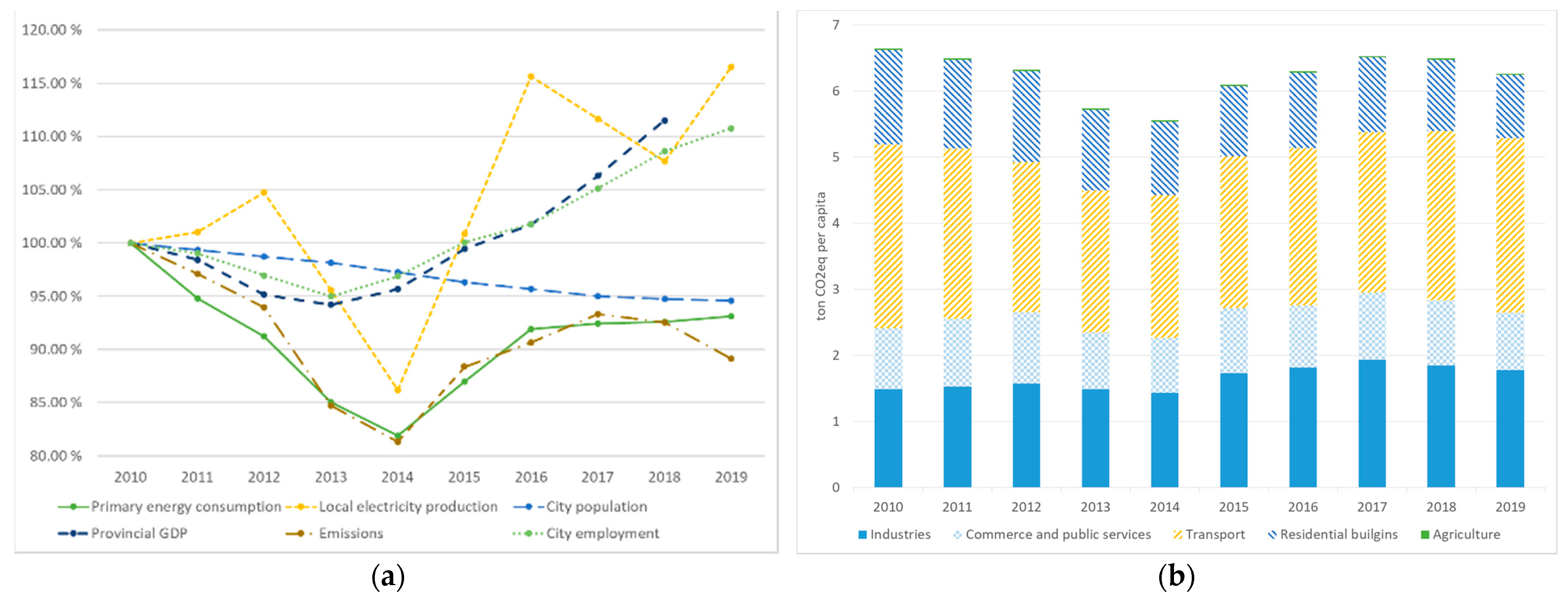
• Energy consumption is strongly linked to economic activity. Even with a population decline trend in our case study city, energy consumption increased from 2015, which is linked to industry, services, and transportation, while even residential consumption increased in the period 2016–2018. The share of energy consumption by sector remains practically constant throughout the decade, although an important fall in residential consumption (a decrease of 28.5%) was detected through the period analysis, while consumption increased in economic activities (an increase of 10.7% in commerce and services and 29.2% of industrial consumption). We should point out that there is an ongoing transformation in household residential consumption that explains these trends, as people spend more in services while avoiding domestic energy consumption. This reduction may be the result of the combination of efficiency policies (which could be a symptom of the rebound effect on household consumption [76]) and energy poverty, which in Spain still remains a serious problem [77]. The disaggregation of the data by income sources may help to shed further light on this issue in the future.
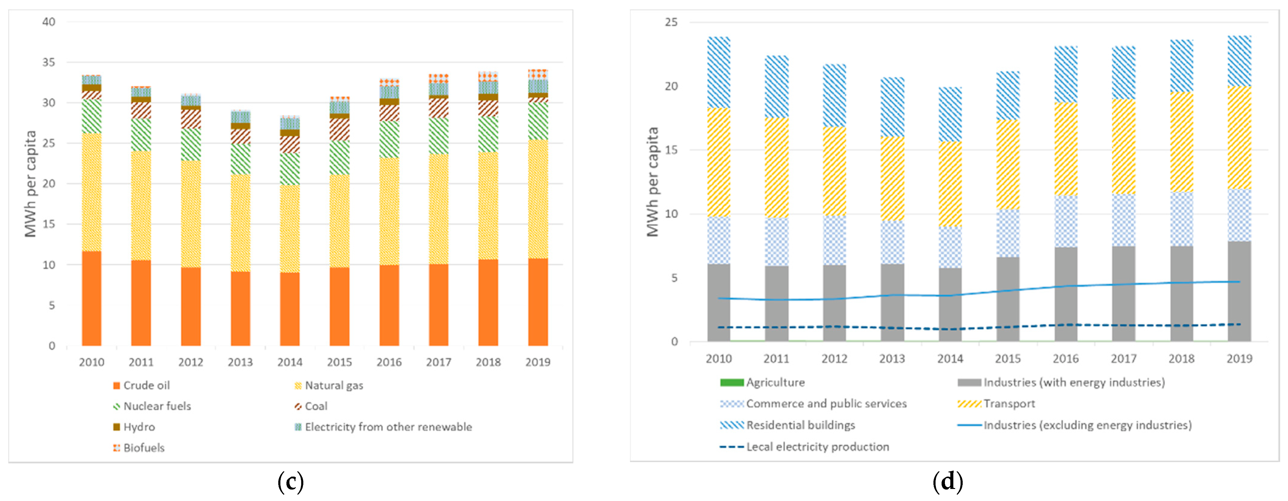
• The sources of the energy consumed remain roughly constant throughout the decade. Despite the numerous institutional strategies [78] and the relative increase in the consumption of biomass (1365% increase from 2010–2019) and photovoltaic solar energy output (228.5% increase from 2010–2019), there is no significant change in the energy consumption pattern (both still below 3% of the total amount of primary energy consumed in 2019). This analysis shows that there has not been an important substitution of energy sources during the period studied, although there are important ongoing efforts that show the high impact that can be obtained if substantially scaled-up in the future (i.e., the University of Valladolid biomass district heating).
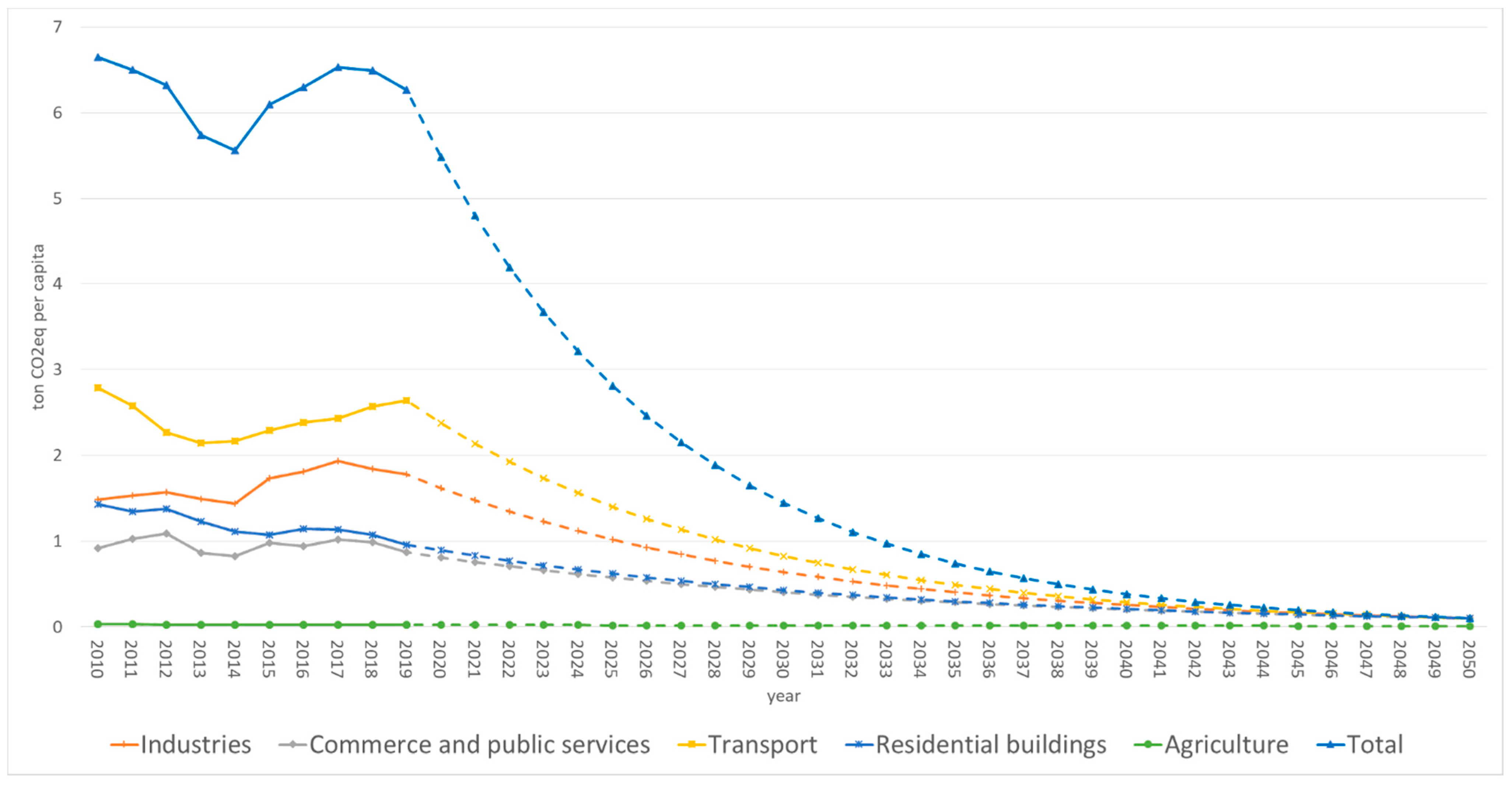
• At local level, the city council has implemented some policies aimed at transitioning to a more sustainable model. We mentioned the SEAP [36], which established a reduction of 20% in GHG emissions. Furthermore, along the decade, the approval of the new urban plan (PGOU) in 2017 [79] stands out because of its effects on land use policies, as a compact city is defined, rejecting the urban sprawl model already in place. This plan proposes a modal shift in urban mobility to low-carbon modes (public transport, bicycle, pedestrian, etc.).

We can now evaluate the results. As is shown, by 2019, the SEAP objectives were not reached, and the reduction in GHG emissions per capita by 2019 were just ~11% lower than the 2010 emissions (vs. a 20% reduction objective). If we exclude the whole industrial sector, the reduction was 14% in 2019 with respect to 2010. In annual terms, the total reduction was 0.6%/year, but with an increasing trend, in the second half of the period studied (2014–2019), there was an increase of +2.2%/year. In fact, the trend in GHG has not been monotone over the period and has instead followed a U-shape, strongly correlated with the economic crisis and the subsequent recovery, suggesting that the transition policies put in place to date had, at most, a modest effect on the overall results.

It has to be taken into account that data for 2020 will be strongly affected by the COVID-19 health crisis and may show a temporary compliance with the objective, due to the reduction in energy consumption during the confinements, economic paralysis, and travel restrictions. However, with the return to the “new normal” and the empirical evidence gathered in this work, a rebound in energy consumption and, hence, GHG emissions seems most likely [80,81].

Following the Paris Agreement (COP21), the regulatory framework sets the objective of achieving carbon neutrality by 2050. The stringency of this objective is represented in Figure 11, assuming an exponential reduction in GHG emission. During the last decade, the reductions in GHG emissions have only occurred in residential buildings (−33%, −4.4%/year) and in agriculture (−18%, −2.2%/year), and these reductions have been partially offset by increases in industry (+20%, +2.1%/year). Reaching GHG neutrality in 2050 requires a reduction in the GHG emissions at a local level of at least ~13% per year (Figure 11), which is 20x faster than the aforementioned 2010–2019 average of 0.6%/year. This explains the annual reduction of −62,300 tonCO₂eq on average between 2020 and 2050 (starting from −242,971 ton CO₂eq annual reduction in 2020 to −3240 ton CO₂eq in 2050). In fact, the only sector that has started a decline consistent with that objective during this decade is the residential buildings sector. Some strategies for reducing energy in buildings have been timidly implemented throughout the decade: the insertion of distributed renewable (solar photovoltaic), biomass district heating, heat pumps, etc. These technologies have an important potential to further reduce the natural gas consumption in the city, especially in residential and tertiary buildings. On the other hand, with the vast industrial zones and the diversity of existing industrial plants, there is potential for the implementation of industrial symbiosis initiatives similar to those existing in other countries [82], and which have been practiced in particular in China over recent decades [83]. How the required rapid decrease in GHG can be achieved remains beyond the scope of the current work, especially given that there are different transition strategies in the scientific debate, such as the most conventional green growth based on technological change and market mechanisms to the more heterodox Green New Deal or postgrowth/degrowth proposals, with a stronger emphasis on the role of the state and/or lifestyle changes and a different economic paradigm [84,85,86].

At the same time, we should point out that the GHG emissions analyzed would be significantly higher (+20–25%) if the fugitive emissions associated with natural gas consumption were accounted for [72].

From the point of view of the geographical boundaries considered, there is evidence in the literature of a higher energy footprint than use of primary energy in rich countries. The existence of a “virtual” transference of energy between countries has been demonstrated through embodied energy in goods exchanged in international trade [87]. For the case of Spain, Arto et al. [87] found that the total primary energy footprint in 2008 was almost 35% higher than the total primary energy demand (with an increasing trend from 1995). Akizu-Gardoki et al. [35] found a hidden energy flow of 24.30% for 2011, taking the EORA database as reference. This is due to the fact that, in the current context of globalization, rich countries have, for decades, systematically outsourced energy-intensive processes to emerging or in-development countries. Hence, the energy used by a country or municipality is no longer a suitable indicator for measuring the total energy requirements associated with its level of development; instead, the significant variable is the energy consumed worldwide to produce the goods and services demanded by that country, i.e., its energy footprint. This hidden energy consumption implies that, in general, for cities in rich countries, as is the case of our case study, the energy consumption of the inhabitants from a consumption-based perspective should be higher than our results obtained here. However, the lack of input–output tables at a municipal level for Valladolid makes it impossible to estimate this indicator for other larger geographical dimensions in the literature [35]. This indicator can be helpful, not only in order to obtain the differences between countries, but also between cities (by size or location) and between urban and non-urban locations.

An option to approximate our results to the consumption-based metric would be to take the aforementioned Spanish average and apply it to the city energy-level calculated in this work (e.g., for the year 2019: 34.07 × (1 + 24.30%) = 42.35 MWh per capita of primary energy consumption in Valladolid). However, two issues arise: (i) our numbers are based on final term estimations, while [35,87] compute primary energy (and the energy efficiency in rich and emerging or in-development countries can be very different); and (ii) the industrial exporter profile of our case study city. Figure 10 shows that Valladolid stands out with respect to other Spanish cities because of its larger energy consumption per capita. Furthermore, it still shows a level that is 10% higher than the country level. In particular, cold winters force more to be spent on heating in Valladolid than in the other locations, although the residential and tertiary buildings do not represent more than 30% of the final energy consumption, that share being higher in Madrid and Valencia [17,18]. On the contrary, the share of final energy consumption in the industrial sector in Valladolid is the largest of the three cases. It is necessary to take into account the fact that Valladolid hosts an important industrial sector destined to export goods: the automotive manufacturing sector in Valladolid exports ~200,000 vehicles/year and ~500,000 engines/year, which, for example, represented 18% of the full regional (Castile-and-Leon) exportation value in 2019 [88]. Hence, all these data suggest that the difference between the territorial and consumption-based energy footprint balance of the city may be less important (or even negative) than the Spanish average, and we consider this topic an issue to be covered in future research.

4.3. Discussion of Methodological Issues

The downscaling factors used to estimate the different energy product imports (Section 2.5.1) show enough accuracy in view of the comparison with other cases (Section 4.1). This estimation risks not capturing the variations in the behavior of the city population with respect to the rest of the province. It is assumed that the energy consumed is proportional to each person or each job, without taking into account that there may be different intensities of use due to different lifestyles (urban-rural) or different industrial energy intensities. On the other hand, it is a reasonable hypothesis, considering that there may not be a great difference in the ways of life or productive processes between the city and the province that may affect energy consumption.

From a methodological point of view, some conclusions can be drawn from the developed method based on bottom-up estimations. As shown, it is possible to obtain accurate estimates for the energy consumption of residential buildings without excessive complexity (2010, Figure 9). Furthermore, there is a lack of accuracy in the time series results, with a growing gap. Taking the energy consumption by surface unit as constant neglects some relevant factors that affect residential buildings. Some of these factors can be modeled, accounting for the rehabilitation investment for each year and how it affects the energy demand. However, there are other factors that can derail the bottom-up estimation, such as behavioral changes. These results must warn us against extending these bottom-up assumptions through a long time series.

The limitations of the data available to characterize energy consumption and GHG emissions due to transport are highlighted. The bottom-up estimates provided indicate that personal mobility accounts for a very small part of the total consumption of oil products for transport. We should note the several problems associated with the information available in this regard, which affects both the energy consumption estimation by downscaling and the bottom-up estimation based on mobility data.

• A lack of data on mobility in the functional urban area. The mobility data available excludes trips between the city and the rest of the urban zones in the functional urban area, which can be an important amount. We consider that this situation is due to the absence of an adequate institutional framework for both the processing of data and the adoption of policies at a metropolitan level.
• The dispersion of fuel suppliers in multiple companies and gas stations make it difficult to allocate the territorial energy consumption. The different fuel supply companies carry out their own internal redistribution under their economic calculations, which are not restricted to administrative limits.
• A lack of information on freight transport. There is a general absence of information about freight distribution at a local level, and not only in the Valladolid case [89,90], which represents an important limitation to achieve a detailed energy consumption characterization.

Considering these limitations, it might be a priority in public policies to obtain better-quality data in these matters, especially for those more concerned with the local level (city council, regional administrations, or even universities). In order to mitigate this problem, public administrations could adopt other data resources, such as geo-localized datasets [91] or the inclusion of systematic freight inventories in a permanent statistical program at the municipal level.

4.4. Further Work

Finally, further work may be oriented towards the comprehensive analysis of the whole urban metabolism of the city of Valladolid, including those dimensions excluded from this analysis, such as the footprints of agricultural products, in order to estimate a more exhaustive set of environmental footprint indicators to complement energy and GHG emissions, such as water or land use. In addition, a better understanding of the energy consumption processes located in the city may allow a deeper analysis of energy end-uses. In that sense, the operational data of the energy plants in the city (CHP, district heating…) would be required. The ongoing energy transition (i.e., the installation of district heating and large renewable plants in the city, the use of natural gas and electricity in transport, and the mobility policies or the energetic efficiency investments) as well as the impact of the COVID crisis should also be analyzed.

5. Conclusions

In conclusion, we point out some specific aspects of our case study and other more general aspects that can be useful for other cities.

We showed that the GHG emissions reduction policies agreed by the city council within the framework of the CoM [36] were not achieved by 2019, as the reduction in GHG emissions in the city were ~11% (reduced to ~5.8% per capita due to a population loss of ~5.5%, i.e., 17,000 inhabitants, in the city over the studied period). This is because energy consumption is very dependent on fossil fuels (natural gas and oil products) in all sectors. The contribution of renewable sources is still very limited (3% with respect to the primary energy consumed in the city in 2019), despite the growth experienced throughout the decade. Regarding particular sectors, the only one that shows a continuous drop in energy consumption is residential buildings, although the analysis performed cannot identify its drivers. We find that reaching GHG neutrality in the city by 2050 would require a reduction in the GHG emissions of ~13%/year, which is ~20x faster the 2010–2019 average of 0.6%/year.

The results show the lack of accuracy of the residential building bottom-up estimation, so we cannot make statements on household consumption in residential buildings. Furthermore, we found serious limitations in analyzing the agents involved in transport energy consumption, which represents a significant consumption share. Our estimates concerning passenger transport explain approximately 20% of the energy consumption in the transport sector, although we must point to significant difficulties in the availability of precise data on mobility.

Overall, there is a lack of sufficiently precise, detailed evidence from data sources at the different relevant institutional levels, and notably at metropolitan level, to accurately analyze the energy flows of the city of Valladolid, which is ultimately a basic requirement for the development of effective policies.

As a synthesis, the main methodological contribution of this case study is the development of a novel methodology which can be useful for other medium or small-size cities. We estimate:

• Local energy consumption based on non-local information sources;
• Household energy consumption based on data from the energy consumption of residential buildings and data of passenger transport, using mobility data.

In order to achieve the objectives set for mitigating climate change, it is necessary to adopt strong measures to understand and transform energy-consuming activities at the local level. We highlight the fact that every GHG ton counts and, therefore, each city, whatever its size, must adopt the necessary measures, acknowledging that these must be set up in a coordinated way by all the relevant institutional levels, particularly those beyond the municipal level, which, in Spain, is ultimately greatly limited by institutional competences and available budget.

References

1. Steffen, W.; Richardson, K.; Rockström, J.; Cornell, S.E.; Fetzer, I.; Bennett, E.M.; Biggs, R.; Carpenter, S.R.; De Vries, W.; De Wit, C.A.; et al. Planetary boundaries: Guiding human development on a changing planet. Science 2015, 347, 1259855. [Google Scholar] [CrossRef] [Green Version]
2. IPCC. Climate Change 2014: Synthesis Report. Contribution of Working Groups I, II and III to the Fifth Assessment Report of the Intergovernmental Panel on Climate Change; Core Writing Team, Pachauri, R., Meyer, L., Eds.; IPCC: Geneva, Switzerland, 2014. [Google Scholar]
3. Millennium Ecosystem Assessment. Ecosystems and Human Well-Being: Synthesis; Island Press: Washington, DC, USA, 2005. [Google Scholar]
4. Trisos, C.H.; Merow, C.; Pigot, A.L. The projected timing of abrupt ecological disruption from climate change. Nature 2020, 580, 496–501. [Google Scholar] [CrossRef]
5. IPCC. Climate Change 2021: The Physical Science Basis. Contribution of Working Group I to the Sixth Assessment Report of the Intergovernmental Panel on Climate Change; Masson-Delmotte, V., Zhai, P., Pirani, A., Connors, S.L., Péan, C., Berger, S., Caud, N., Chen, Y., Goldfarb, L., Gomis, M.I., et al., Eds.; Cambridge University Press: Cambridge, UK, 2021; in press. [Google Scholar]
6. Ivanova, D.; Wood, R. The unequal distribution of household carbon footprints in Europe and its link to sustainability. Glob. Sustain. 2020, 3, e18. [Google Scholar] [CrossRef]
7. Wiedmann, T.; Lenzen, M.; Keyßer, L.T.; Steinberger, J.K. Scientists’ warning on affluence. Nat. Commun. 2020, 11, 1–10. [Google Scholar] [CrossRef]
8. IPCC. Climate Change 2007: Synthesis Report. Contribution of Working Groups I, II and III to the Fourth Assessment Report of the Intergovernmental Panel on Climate Change; Core Writing Team, Pachauri, R.K., Reisinger, A., Eds.; IPCC: Geneva, Switzerland, 2007. [Google Scholar]
9. Nieto, J.; Carpintero, Ó.; Miguel, L.J. Less than 2 °C? An Economic-Environmental Evaluation of the Paris Agreement. Ecol. Econ. 2018, 146, 69–84. [Google Scholar] [CrossRef]
10. Keivani, R. A review of the main challenges to urban sustainability. Int. J. Urban Sustain. Dev. 2010, 1, 5–16. [Google Scholar] [CrossRef]
11. Martos, A.; Pacheco-Torres, R.; Ordóñez, J.; Jadraque-Gago, E. Towards successful environmental performance of sustainable cities: Intervening sectors. A review. Renew. Sustain. Energy Rev. 2016, 57, 479–495. [Google Scholar] [CrossRef]
12. Reckien, D.; Salvia, M.; Heidrich, O.; Church, J.M.; Pietrapertosa, F.; De Gregorio-Hurtado, S.; D’Alonzo, V.; Foley, A.; Simoes, S.G.; Krkoška Lorencová, E.; et al. How are cities planning to respond to climate change? Assessment of local climate plans from 885 cities in the EU-28. J. Clean. Prod. 2018, 191, 207–219. [Google Scholar] [CrossRef]
13. CoM Covenant of Mayors. Available online: https://www.covenantofmayors.eu/ (accessed on 30 June 2021).
14. Reckien, D.; Flacke, J.; Olazabal, M.; Heidrich, O. The influence of drivers and barriers on urban adaptation and mitigation plans-an empirical analysis of European Cities. PLoS ONE 2015, 10, e0135597. [Google Scholar] [CrossRef]
15. Grubler, A.; Bai, X.; Buettner, T.; Dhakal, S.; Fisk, D.; Ichinose, T.; Keirstead, J.; Sammer, G.; Satterthwaite, D.; Schulz, N.; et al. Chapter 18: Urban energy systems. In Global Energy Assessment: Toward a Sustainable Future; Cambridge University Press: Cambridge, UK, 2012; pp. 1307–1400. [Google Scholar]
16. Baynes, T.; Bai, X. Trajectories of Change: Melbourne’s Population, Urban Development, Energy Supply and Use from 1960–2006; International Institute for Applied Systems Analysis (IIASA): Laxenburg, Austria, 2006. [Google Scholar]
17. Pérez, J.; Lázaro, S.; Lumbreras, J.; Rodríguez, E. A methodology for the development of urban energy balances: Ten years of application to the city of Madrid. Cities 2019, 91, 126–136. [Google Scholar] [CrossRef]
18. Muñoz, I.; Hernández, P.; Pérez-Iribarren, E.; Pedrero, J.; Arrizabalaga, E.; Hermoso, N. Methodology for integrated modelling and impact assessment of city energy system scenarios. Energy Strateg. Rev. 2020, 32, 100553. [Google Scholar] [CrossRef]
19. Abbasabadi, N.; Ashayeri, M.; Azari, R.; Stephens, B.; Heidarinejad, M. An integrated data-driven framework for urban energy use modeling (UEUM). Appl. Energy 2019, 253, 113550. [Google Scholar] [CrossRef]
20. Fichera, A.; Inturri, G.; La Greca, P.; Palermo, V. A model for mapping the energy consumption of buildings, transport and outdoor lighting of neighbourhoods. Cities 2016, 55, 49–60. [Google Scholar] [CrossRef]
21. Osório, B.; McCullen, N.; Walker, I.; Coley, D. Integrating the energy costs of urban transport and buildings. Sustain. Cities Soc. 2017, 32, 669–681. [Google Scholar] [CrossRef]
22. Osório, B. Characterizing the Relationship between Energy and Urban Form Using Data, Scaling and Combined Metrics. Doctoral Dissertation, University of Bath, Bath, UK, November 2017. [Google Scholar]
23. Carre, R.; Wegener, A. Exploring urban metabolism—Towards an interdisciplinary perspective. Resour. Conserv. Recycl. 2018, 132, 190–203. [Google Scholar] [CrossRef]
24. Kennedy, C.; Pincetl, S.; Bunje, P. The study of urban metabolism and its applications to urban planning and design. Environ. Pollut. 2011, 159, 1965–1973. [Google Scholar] [CrossRef]
25. Giampietro, M.; Mayumi, K.; Ramos-Martin, J. Multi-scale integrated analysis of societal and ecosystem metabolism (MuSIASEM): Theoretical concepts and basic rationale. Energy 2009, 34, 313–322. [Google Scholar] [CrossRef]
26. Pérez-Sánchez, L.; Giampietro, M.; Velasco-Fernández, R.; Ripa, M. Characterizing the metabolic pattern of urban systems using MuSIASEM: The case of Barcelona. Energy Policy 2019, 124, 13–22. [Google Scholar] [CrossRef]
27. García-Guaita, F.; González-García, S.; Villanueva-Rey, P.; Moreira, M.T.; Feijoo, G. Integrating Urban Metabolism, Material Flow Analysis and Life Cycle Assessment in the environmental evaluation of Santiago de Compostela. Sustain. Cities Soc. 2018, 40, 569–580. [Google Scholar] [CrossRef]
28. González-García, S.; Dias, A.C. Integrating lifecycle assessment and urban metabolism at city level: Comparison between Spanish cities. J. Ind. Ecol. 2019, 23, 1062–1076. [Google Scholar] [CrossRef]
29. Rama, M.; González-García, S.; Andrade, E.; Moreira, M.T.; Feijoo, G. Assessing the sustainability dimension at local scale: Case study of Spanish cities. Ecol. Indic. 2020, 117, 106687. [Google Scholar] [CrossRef]
30. Heinonen, J.; Ottelin, J.; Ala-Mantila, S.; Wiedmann, T.; Clarke, J.; Junnila, S. Spatial consumption-based carbon footprint assessments—A review of recent developments in the field. J. Clean. Prod. 2020, 256, 120335. [Google Scholar] [CrossRef]
31. Chen, G.; Shan, Y.; Hu, Y.; Tong, K.; Wiedmann, T.; Ramaswami, A.; Guan, D.; Shi, L.; Wang, Y. Review on City-Level Carbon Accounting. Environ. Sci. Technol. 2019, 53, 5545–5558. [Google Scholar] [CrossRef]
32. Nangini, C.; Peregon, A.; Ciais, P.; Weddige, U.; Vogel, F.; Wang, J.; Bréon, F.-M.; Bachra, S.; Wang, Y.; Gurney, K.; et al. Data Descriptor: A global dataset of CO 2 emissions and ancillary data related to emissions for 343 cities. Sci. Data 2019, 6, 180280. [Google Scholar] [CrossRef] [PubMed]
33. Harris, S.; Weinzettel, J.; Bigano, A.; Källmén, A. Low carbon cities in 2050? GHG emissions of European cities using production-based and consumption-based emission accounting methods. J. Clean. Prod. 2020, 248, 119206. [Google Scholar] [CrossRef]
34. Lenzen, M.; Dey, C.; Foran, B. Energy requirements of Sydney households. Ecol. Econ. 2004, 49, 375–399. [Google Scholar] [CrossRef]
35. Akizu-Gardoki, O.; Wakiyama, T.; Wiedmann, T.; Bueno, G.; Arto, I.; Lenzen, M.; Lopez-Guede, J.M. Hidden Energy Flow indicator to reflect the outsourced energy requirements of countries. J. Clean. Prod. 2021, 278, 123827. [Google Scholar] [CrossRef]
36. Ayuntamiento de Valladolid. Sustainable Energy Action Plan; Ayuntamiento de Valladolid: Valladolid, Spain, 2010. [Google Scholar]
37. Eurostat. Methodological Manual on Territorial Typologies; Publications Office of the European Union: Luxemburg, 2018. [Google Scholar]
38. OEDC. OECD Regions at a Glance 2016; OECD Publishing: Paris, France, 2016; ISBN 9789264252097. [Google Scholar]
39. United Nations Statistics Division. International Recommendations for Energy Statistics (IRES); United Nations: New York, NY, USA, 2018; ISBN 9789211615845. [Google Scholar]
40. Swan, L.G.; Ugursal, V.I. Modeling of end-use energy consumption in the residential sector: A review of modeling techniques. Renew. Sustain. Energy Rev. 2009, 13, 1819–1835. [Google Scholar] [CrossRef]
41. Sede Electrónica del Catastro Cadastral Data Difussion. Available online: https://www.sedecatastro.gob.es/Accesos/SECAccDescargaDatos.aspx (accessed on 29 June 2021).
42. Pérez, J.; de Andrés, J.M.; Borge, R.; de la Paz, D.; Lumbreras, J.; Rodríguez, E. Vehicle fleet characterization study in the city of Madrid and its application as a support tool in urban transport and air quality policy development. Transp. Policy 2019, 74, 114–126. [Google Scholar] [CrossRef]
43. Ayuntamiento de Valladolid Valladolid Urban Observatoy. Available online: http://www.valladolidencifras.es/ (accessed on 29 June 2021).
44. Instituto Nacional de Estadística Population and Housing Census. 2011. Available online: https://www.ine.es/censos2011_datos/cen11_datos_inicio.htm (accessed on 29 June 2021).
45. De las Rivas, J.; Alvarez, A.; Paris, M. El corredor industrial Valladolid-Palencia: Conurbación emergente entre dos polos urbanos consolidados. Ciudad Territ. Estud. Territ. 2013, XLV, 352–363. [Google Scholar]
46. REBI SLU Univerisity of Valladolid Distric Heating. Available online: https://recursosdelabiomasa.es/redes-de-calor/red-de-calor-de-la-universidad-de-valladolid (accessed on 30 June 2021).
47. Junta de Castilla y León Statistical Information System—Sistema de Información Estadística (SIE). Available online: https://www.jcyl.es/sie/sas/broker?_PROGRAM=mddbpgm.v2.indexv2.scl&_SERVICE=saswebl&_DEBUG=0&menu=cuentascotiz (accessed on 29 June 2021).
48. Ministerio para la Transición Ecológica y el Reto Demográfico Publicaciones Estadísticas. Available online: https://energia.gob.es/balances/Publicaciones/Paginas/Publicaciones_estadisticas.aspx (accessed on 29 June 2021).
49. CORES Statistics. Available online: https://www.cores.es/es/estadisticas (accessed on 29 June 2021).
50. Ayuntamiento de Valladolid Sustainable Energy Action Plan Reports. Available online: https://www.valladolid.es/es/temas/hacemos/agencia-energetica-municipal-aemva/inventario-emisiones (accessed on 29 June 2021).
51. Junta de Castilla y León DATAHUB of Energy Statistics of Castilla-y-Leon Regional Administration. Available online: https://analisis.datosabiertos.jcyl.es/pages/eren/?flg=es#centros-de-consumo (accessed on 29 June 2021).
52. Junta de Castilla y León. Autorización Ambiental Energyworks Vit-Vall, S.L., Para Planta de Cogeneración de 77,8 MW. Térmicos, en las Instala-Ciones de Michelín España-Portugal, S.A.; Junta de Castilla y León: Valadolid, Spain, 2009; pp. 1338–1347. [Google Scholar]
53. PRTR España Informe Detallado Energyworks Vitvall S.L. Available online: https://prtr-es.es/informes/fichacomplejo.aspx?Id_Complejo=3180 (accessed on 29 June 2021).
54. Aquavall. Informe de sostenibilidad 2019; Aquavall: Valladolid, Spain, 2019. [Google Scholar]
55. Ayuntamiento de Valladolid, Pliego Prescripciones Técnicas Contrato CTR Valladolid; Ayuntamiento de Valladolid: Valladolid, Spain, 2018.
56. Ministerio Para la Transición Ecológica Registro Administrativo de Instalaciones de Producción de Energía Eléctrica. Available online: https://energia.serviciosmin.gob.es/Pretor/ (accessed on 30 June 2021).
57. IDAE; Ayuntamiento de Valladolid, Análisis de Movilidad. PIMUSSVA; Ayuntamiento de Valladolid: Valladolid, Spain, 2015. [Google Scholar]
58. OTLE. Study of Interprovincial Mobility of Travelers applying Big Data Technology. Available online: https://observatoriotransporte.mitma.es/estudio-experimental (accessed on 29 June 2021).
59. Bettencourt, L.M.A. A unified theory of urban living. Nature 2010, 467, 912–913. [Google Scholar] [CrossRef]
60. Youn, H.; Lobo, J.; Bettencourt, L.M.A. The hypothesis of urban scaling: Formalization, implications and challenges. arXiv 2013, arXiv:1301.5919. [Google Scholar]
61. Bettencourt, L.M.A. The Origins of Scaling in Cities. Science 2013, 340, 1438–1441. [Google Scholar] [CrossRef] [Green Version]
62. Arbabi, H.; Mayfield, M. Urban and rural-population and energy consumption dynamics in local authorities within England and Wales. Buildings 2016, 6, 34. [Google Scholar] [CrossRef] [Green Version]
63. ESIOS Maps. Available online: https://www.esios.ree.es/es/mapas-de-interes (accessed on 29 June 2021).
64. Prussi, M.; Yugo, M.; De Prada, L.; Padella, M.; Edwards, R.; Lonza, L. JEC Well-To-Tank Report v5; Publications Office of the European Union: Luxembourg, 2020. [Google Scholar]
65. Red Eléctrica de España Spanish Electrical System Report 2019. Available online: https://www.ree.es/es/datos/publicaciones/informe-anual-sistema/informe-del-sistema-electrico-espanol-2019 (accessed on 29 June 2021).
66. Ministerio para la Transición Ecológica y el Reto Demográfico. Informe de inventario nacional de Gases de Efecto Invernadero. Comunicación a la Comisión Europea del Reglamenteo (UE) no525/2013. Comunicación al Secretariado de la Convención Marco de las Naciones Unidas sobre el Cambio Climático. Edición 2021 (1990–2019); Ministerio para la Transición Ecológica y el Reto Demográfico: Madrid, Spain, 2021.
67. González, M.C.; Hidalgo, C.A.; Barabási, A.L. Understanding individual human mobility patterns. Nature 2008, 453, 779–782. [Google Scholar] [CrossRef]
68. Ministerio de Industria, E.y.T.; Ministerio de Fomento. Factores de Emisión de CO2 y Coeficientes de Paso a Energía Primaria de Diferentes Fuentes de Energía Final Consumidas en el Sector de Edificios en España; Ministerio de Industria, E.y.T: Madrid, Spain, 2016.
69. OTLE. 2017 Annual Report; Ministerio de Fomento: Madrid, Spain, 2018.
70. IDAE. Labelling schemes for New Buildings (Translated from Spanish Original); IDAE: Madrid, Spain, 2009. [Google Scholar]
71. IDAE. Project Sech-Spahousec, Analysis of the Energetic Consumption of the Residential Sector in Spain (Proyecto Sech-Spahousec, Análisis del Consumo Energético del Sector Residencial en España); IDAE: Madrid, Spain, 2016. [Google Scholar]
72. Howarth, R.W. A bridge to nowhere: Methane emissions and the greenhouse gas footprint of natural gas. Energy Sci. Eng. 2014, 2, 47–60. [Google Scholar] [CrossRef]
73. World Energy Balances—Data Product—IEA. Available online: https://www.iea.org/data-and-statistics/data-product/world-energy-balances (accessed on 21 July 2021).
74. Manzanera-Benito, G. Evaluación del Sistema Movilidad-Territorio en el Área Funcional de Valladolid; Universidad de Valladolid: Valladolid, Spain, 2019. [Google Scholar]
75. Lomas, P.L.; Carpintero, Ó. Metabolismo y huella ecológica de la alimentación: El caso de Valladolid; Universidad de Valladolid: Valladolid, Spain, 2017. [Google Scholar]
76. Chitnis, M.; Sorrell, S.; Druckman, A.; Firth, S.K.; Jackson, T. Who rebounds most? Estimating direct and indirect rebound effects for different UK socioeconomic groups. Ecol. Econ. 2014, 106, 12–32. [Google Scholar] [CrossRef] [Green Version]
77. Ministerio para la Transición Ecológica y el Reto Demográfico. Actualización de Indicadores de la Estrategia Nacional Contra la Pobreza Energética. Noviembre 2020; Ministerio para la Transición Ecológica y el Reto Demográfico: Madrid, Spain, 2020.
78. De las Rivas Sanz, J.L.; Fernández-Maroto, M. Strategy for Energy Transition in the Cities of Castile and Leon. Base Document; de Castilla y León, J., Universidad de Valladolid. Instituto Universitario de Urbanística, Eds.; Universidad de Valladolid: Valladolid, Spain, 2021. [Google Scholar]
79. Ayuntamiento de Valladolid PGOU 2020. Available online: https://www.valladolid.es/es/temas/hacemos/aprobacion-definitiva-pgou-2020 (accessed on 30 June 2021).
80. Prol, J.L.; Sungmin, O. Impact of COVID-19 Measures on Short-Term Electricity Consumption in the Most Affected EU Countries and USA States. iScience 2020, 23, 101639. [Google Scholar] [CrossRef]
81. Gualtieri, G.; Brilli, L.; Carotenuto, F.; Vagnoli, C.; Zaldei, A.; Gioli, B. Quantifying road traffic impact on air quality in urban areas: A Covid19-induced lockdown analysis in Italy. Environ. Pollut. 2020, 267, 115682. [Google Scholar] [CrossRef]
82. Jacobsen, N.B. Industrial symbiosis in Kalundborg, Denmark: A quantitative assessment of economic and environmental aspects. J. Ind. Ecol. 2006, 10, 239–255. [Google Scholar] [CrossRef]
83. Neves, A.; Godina, R.; Azevedo, S.G.; Matias, J.C.O. A comprehensive review of industrial symbiosis. J. Clean. Prod. 2020, 247, 119113. [Google Scholar] [CrossRef]
84. Mastini, R.; Kallis, G.; Hickel, J. A Green New Deal without growth? Ecol. Econ. 2021, 179, 106832. [Google Scholar] [CrossRef]
85. Grubler, A.; Wilson, C.; Bento, N.; Boza-Kiss, B.; Krey, V.; McCollum, D.L.; Rao, N.D.; Riahi, K.; Rogelj, J.; De Stercke, S.; et al. A low energy demand scenario for meeting the 1.5 °C target and sustainable development goals without negative emission technologies. Nat. Energy 2018, 3, 515–527. [Google Scholar] [CrossRef]
86. Millward-Hopkins, J.; Steinberger, J.K.; Rao, N.D.; Oswald, Y. Providing decent living with minimum energy: A global scenario. Glob. Environ. Chang. 2020, 65, 102168. [Google Scholar] [CrossRef]
87. Arto, I.; Capellán-Pérez, I.; Lago, R.; Bueno, G.; Bermejo, R. The energy requirements of a developed world. Energy Sustain. Dev. 2016, 33, 1–13. [Google Scholar] [CrossRef] [Green Version]
88. Junta de Castilla y León Statistics on External Trade and Intra-EU Trade 2014–2019. Available online: https://estadistica.jcyl.es/web/jcyl/Estadistica/es/Plantilla100Detalle/1284785305778/Publicacion/1285022602339/Redaccion (accessed on 30 July 2021).
89. Muñuzuri, J.; Cortés, P.; Onieva, L.; Guadix, J. Modelling peak-hour urban freight movements with limited data availability. Comput. Ind. Eng. 2010, 59, 34–44. [Google Scholar] [CrossRef]
90. Muñuzuri, J.; Grosso, R.; Escudero, A.; Cortés, P. Distribución de mercancías y desarrollo urbano sostenible. Rev. Transp. Territ. 2017, 17, 34–58. [Google Scholar]
91. Barbosa, H.; Barthelemy, M.; Ghoshal, G.; James, C.R.; Lenormand, M.; Louail, T.; Menezes, R.; Ramasco, J.J.; Simini, F.; Tomasini, M. Human mobility: Models and applications. Phys. Rep. 2018, 734, 1–74. [Google Scholar] [CrossRef] [Green Version]
Figure 1. Overview of the workflow towards estimating the energy flows and GHG of the medium-size city of Valladolid.
Sustainability 13 13181 g001
Figure 2. Conceptual diagram of energy flows involved in the area.
Sustainability 13 13181 g002
Figure 3. Valladolid province and its municipalities. Own edition with [44] data.
Sustainability 13 13181 g003
Figure 4. GHG emissions by final energy consumption unit.
Sustainability 13 13181 g004
Figure 5. Temporal results. (a) Evolution of main indicators with relation to 2010 in %. (b) GHG year emissions by sector (ton CO2eq per capita). (c) TES by year and energy source (MWh per capita). (d) Final energy consumption by year and sector and local energy production (losses are excluded) (MWh per capita).
Sustainability 13 13181 g005aSustainability 13 13181 g005b
Figure 6. Local electricity production by source.
Sustainability 13 13181 g006
Figure 7. Sankey diagram of energy flows from upstream primary energy products (left side), energy imports (center) and final energy consumption by end-use sector (right) and losses. All percentages over the TES.
Sustainability 13 13181 g007
Figure 8. Comparison between transport top-down final energy consumption (blue bars) and bottom-up personal urban and interurban mobility energy consumption (orange and grey lines).
Sustainability 13 13181 g008
Figure 9. Residential buildings final energy consumption comparison: bottom-up estimation vs. physical flow data.
Sustainability 13 13181 g009
Figure 10. (a) Comparison between final energy consumption per capita by energy product (MWh per capita) in three Spanish cities. (b) Comparison of TES per capita by energy product (MWh per capita) in Valladolid and in Spain along the decade (2019 Spanish TES data are provisional).
Sustainability 13 13181 g010
Figure 11. GHG emissions: historical data (2010–2019) and reduction pathways by sector assuming an exponential decrease.
Sustainability 13 13181 g011