Article

Tourism and Road Transport Emissions in Italy

1
University of Rome “La Sapienza”, 00185 Rome, Italy
2
ISPRA—Italian Institute for Environment Protection and Research, 00144 Rome, Italy
3
ISTAT—Italian National Institute of Statistics, 00184 Rome, Italy
4
Department of Political Sciences, University of Genova, 16124 Genova, Italy
*
Author to whom correspondence should be addressed.
Sustainability 2021, 13(22), 12712; https://doi.org/10.3390/su132212712
Submission received: 29 September 2021 / Revised: 4 November 2021 / Accepted: 11 November 2021 / Published: 17 November 2021
(This article belongs to the Special Issue Indicators of Social Sustainability and Wellbeing)

Abstract

:
Tourism is of great importance to European economies, but environmental degradation could reduce the attractiveness of many European destinations considerably. This is even more evident if the future of tourism is depicted in the UN’s Agenda 2030 for Sustainable Development. However, official statistics on the environmental impact of tourism provide only partial information, and almost always with an “accounting scheme” approach, such as occasional and experimental experiences on integrated economic and environmental accounts of tourism. It is necessary to enrich the activity of monitoring and measuring the impact of tourism on the environment and implement policies aimed at increasing the sustainability of the sector. This work intends to contribute to extending information about the theme, providing a new approach based on the integration of official data to study the relationship between tourism and the environment. In detail, the objective of the work is to estimate the level of emissions—in terms of the primary air pollutants—produced by tourists travelling in Italy by road transport in the period 2015–2019. Even if much has to be done to improve the knowledge on the tourism–environment nexus, this paper represents a first relevant step towards an approach that can be easily implemented in all EU countries.

1. Introduction

The awareness that tourism may heavily affect the environment was reached many years ago [1,2], becoming one of the main topics in the growing green economy. The last G20 Tourism Ministers meeting on the 4th of May 2021, after the COVID-19 pandemic, welcomed the Recommendations for the Transition to a Green Travel and Tourism Economy [3]. However, the measurement of this impact is still almost “unknown” to official national statistical offices. Due to the difficulties of measuring the phenomenon directly, it is necessary to find alternative indicators. This work’s central hypothesis and motivation are that it is possible to produce environmental tourism indicators using already available official statistical data used to fulfil other purposes than measuring the environmental impact of tourism. By following this assumption, a new methodology is developed and proposed in the next section.
Tourism is generally seen as a productive sector dedicated to creating income, and the statistics available on tourism are essentially designed to measure the economic role of tourism, whereas its effects on the environment are not truly systematically measured [4,5,6]. However, the environmental impact of tourism is receiving more and more attention in the general framework of the Sustainable Development Goals (SDGs) and Agenda 2030. Tourism can contribute directly or indirectly to all of the SDGs, but three, in particular, are recalled herein. In Goal 8, “Decent work and economic growth”, tourism is considered one of the driving forces of global economic growth, as recognized in Target 8.9: “By 2030, devise and implement policies to promote sustainable tourism that creates jobs and promotes local culture and products”. In Goal 12, “Responsible consumption and production”, it is made evident that the tourism sector can play a significant role in accelerating the global shift towards sustainability by adopting sustainable consumption and production (SCP) practices, as set out in Target 12.b: “Develop and implement tools to monitor sustainable development impacts for sustainable tourism which creates jobs, promotes local culture and products”. In Goal 13, “Climate Action”, it is made evident that tourism contributes to and is affected by climate change. As reported by the World Tourism Organization of the United Nations (UNWTO), “The tourism sector is highly vulnerable to climate change and at the same time contributes to the emission of greenhouse gases (GHG), which cause global warming. Accelerating climate action in tourism is therefore of utmost importance for the resilience of the sector” [7]. A serious concern about this issue was expressed by the UNWTO because “according to UNWTO/ITF latest research (https://www.unwto.org/sustainable-development/tourism-emissions-climate-change, accessed on 22 October 2021) [8], released in December 2019 [9], CO2 emissions from tourism are forecasted to increase by 25% by 2030 from 2016 levels”. The UNWTO also promotes the acceleration “towards low carbon tourism development and the contribution of the sector to international climate goals, in line with the recommendations of the One Planet Vision (https://www.unwto.org/covid-19-oneplanet-responsible-recovery-initiatives, accessed on 22 October 2021) for a Responsible Recovery of the Tourism Sector from COVID-19” [10]. In line with this intention, in the next UNFCC COP26, which will be held in Glasgow in November 2021, the Glasgow Declaration on Climate Action in Tourism [11] will be launched, developed within the framework of the Sustainable Tourism Programme of the One Planet network, which has the ambitious role of ensuring “strong actions and commitment from the tourism sector prior to the COP and beyond, to cut tourism emissions at least in half over the next decade and reach Net Zero emissions as soon as possible before 2050”.
In addition, Goal 14 of the SDGs, “Life below water”, points out Target 14.7: “increase the economic benefits to Small Island developing States and least developed countries from the sustainable use of marine resources, including through sustainable management of fisheries, aquaculture and tourism”.
It is, therefore, in the sector’s interest to play a leading role in the global response to climate change. This work devotes its attention to the abovementioned SDGs and international actions undertaken in this field by proposing a new way to measure and monitor the environmental effects of tourism in a defined area of interest—air pollution. This is the first attempt in Italy and, to the best of our knowledge, in the literature, to combine the information coming from two distinct official data sources for such a purpose.
Official European and national statistical offices need to update the informative sets to account for this new perspective because, both at European and national levels, tourism statistics and environmental statistics are not integrated, despite the indications at the international level (United Nations World Tourism Organization, UNWTO) to use the System of Environmental-Economic Accounting (SEEA) based on a satellite account for tourism, carried out occasionally at the national level (since 2015, ISTAT has regularly published TSAs every two years, in compliance with EU methodology [12]). In fact, ISTAT has created the integrated economic and environmental account of tourism, from time to time, as part of the Measuring the Sustainability of Tourism (MST) project, started in 2015 by the UNWTO. The measurement of the environmental pressures of tourism, starting from the integration of existing accounting schemes, tourism and environment satellite account and environmental–economic accounts, is one of the main objectives of this MST project. In 2019, even if on an experimental basis, it estimated emissions from the National Accounts Matrix, including Environmental Accounts (NAMEA), among the negative environmental externalities [13].
However, to focus entirely on the SEEA, which is consistent with the National Accounting System (SNA) and not with “purely environmental” data from environmental monitoring activities or environmental statistics, means, on the one hand, an extreme predominance of the economic language to the detriment of the truly environmental one; on the other hand, it means approaching the topic in its entirety—that is, speaking about the complete potential tourist economic system. To address this informative gap relating to the availability of primary data, helpful in detecting this nexus between tourism and the environment, ISPRA—the Italian Institute for Environment Protection and Research—and ISTAT—the Italian National Institute of Statistics—signed in 2018 a protocol dedicated to strengthening relationships, already existing in the SISTAN—the Italian System of Official Statistics—in order to define a common scope of action on tourism and the environment. The objective, from the tourism point of view, is the implementation of pilot studies applied to specific territorial areas, aiming to devise statistical indicators related to “Tourism and the Environment”, such as indicators of the pressure and environmental impacts of/on tourism.
As a first step in this “tourism activity” in the protocol mentioned above, the questionnaire of the 2020 edition of the ISTAT’s “Trips and Holidays” (in Italian: “Viaggi e Vacanze”) survey was extended with two additional questions investigating the “type of fuel” and the “cylinder capacity class” of the vehicle used as primary means of transport during a trip or a same-day visit in the case of private motor vehicles (car, motorhome, motorbike, scooter, van, lorry, truck, etc.).
As a secondary output, this paper explains the process and provides the results of an ISPRA–ISTAT joint attempt to estimate the level of emissions in terms of primary atmospheric pollutants produced by private road transport for domestic tourism trips in Italy during the period 2015–2019. This attempt was made by combining the municipal origin-destination distances matrix provided by the ISTAT’s “Trips and Holidays” survey and the ISPRA’s database on the average emission factors by means of road transport, all using two official statistical sources, not “caged” in an accounting approach, but one aimed at tourism aspects and the other at environmental monitoring. In other words, this work contributes to filling the gap in the measurement process of polluting emissions in the global tourism system that must be wholly decarbonized in the next 30 years, in line with other economic sectors. The methodology proposed in the following could be considered a best practice for the other European Member States since tourism data are under European Regulation [14] and environmental data are regulated in the United Nations Economic Commission for Europe (UNECE) framework [15,16]. To meet the global climate change stabilization goals, governments must make a medium- to long-term system-wide commitment to a low-carbon economy transition [17,18,19,20].
Moreover, given the climate emergency, tourism destination managers must seek ways to gain all available efficiencies to ramp down tourism carbon emissions [21] immediately in the short term. New destinations management models are required to move to a tourism paradigm that accounts for the carbon footprint of tourism revenues. It is generally acknowledged that several tourism subsectors, specifically transportation (and, in our application, we focused on road transport), face great difficulties in reducing emissions due to interrelated reasons of rapid growth, their energy intensity and the high cost of technology change [22,23]. However, tourism stakeholders have ignored this emerging problem over several decades and pursued volume growth strategies, with little or no attention being paid to the implications for climate change [24]. Such strategies have created vulnerabilities, including environmental externalities that now must be accounted for [25]. We hope that the draft Glasgow Declaration on Climate Action in Tourism will raise awareness and decisively engage policymakers.
The rest of the paper is organized as follows: in Section 2, we describe the data sources that we used for this study and how they were integrated for the following analysis; in Section 3, we provide the results of the national and the regional analyses, and in Section 4, we discuss the results.

2. Materials and Methods

The primary statistical source of information for tourism flows in Italy is the household sample survey “Trips and Holidays” conducted by ISTAT. From 1997 to 2013, the survey "Trips and Holidays" was a stand-alone survey carried out quarterly using the CATI technique and included in the Multiscope Survey system; since 2014, the survey has become a focus of the household budget sample survey, carried out using the CAPI technique, becoming a continuous survey, carried out every month of the year (see, for details, [26]). (This survey has been carried out regularly since 1997 in compliance, until 2011, with European Directive 95/57/EC and, since 2012, in compliance with European Regulation 692/2011 on tourism statistics.) The survey satisfies the twofold need to guarantee, at a national level, the availability of an integrated system of statistical information on tourism, complementary to that which makes up the tourism supply-side (“Capacity of collective accommodation establishments” and “Occupancy in collective accommodation establishments” by ISTAT) and, at a European level, a wealth of information harmonized among Member States of the European Union. According to international definitions [27,28], tourism flows do not include travel within the municipality where one lives or travel related to one’s daily life and habits if carried out weekly, even outside one’s residential municipality. The aim of the survey is, therefore, to quantify the (non-usual) tourism (adhering to the definitions adopted at an international level, tourism is defined as “all the activities and services relating to people who move outside their ‘usual environment’, for personal or business reasons”) flows of Italian residents, both within the country and abroad, giving official estimates of the number of trips, overnight stays, tourists and same-day visits (daily visits without overnight stays) made during the year, and to estimate travel typologies and tourism behaviors. The range of information includes the main qualitative variables describing a trip (or a same-day visit), such as the destination, the purpose of the travel, the means of booking, the means of transport, the type of accommodation used, the length of stay, the period of the year when residents travel and, finally, the reasons that people did not travel. In addition to these, it provides information on the socio-demographic characteristics of tourists and non-tourists, along with economic information on household expenditure during travels or same-day visits (Survey and methodological insights in [29]). Given the sample nature of the survey, to obtain estimates for the whole population (resident households), it is necessary to use appropriate coefficients to report the subset of the units of the population included in the sample to the complementary subset consisting of the remaining units of the population. The calculation of coefficients is a generalized procedure based on the use of a class of estimators known in the literature as calibration estimators [30].
The reference dataset for calculating the new indicators on pollutant emissions is composed of a subset of trips with overnight stays made within national borders, by which private road transport was the primary means of travel. The dataset includes all types of tourism trips, both for personal reasons and for business. Overall, private motorized vehicles have always been the most widely used means of transport for domestic trips. Specifically, the following categories of means were considered:
  • Rented cars;
  • Private cars, such as relatives’/friends’ cars;
  • Motorhomes, caravans;
  • Motorbikes, scooters, mopeds;
  • Other (vans, lorries, trucks, etc.).
The analysis excluded coaches and buses as they do not fit within the category of private road transport used by tourists on their own, whereas the “other” category refers mainly to business trips made by workers driving vans, lorry trucks and similar means of transport.
The descriptive analysis of the variability of the two datasets of pollutants and trips over the five years considered (from 2015 to 2019) found that the estimates have acceptable yearly fluctuations. The coefficients of variation (CV) (The coefficient of variation (CV), also known as relative standard deviation (RSD), is a standardized measure of the dispersion of a probability distribution or frequency distribution. It is often expressed as a percentage, and is defined as the ratio of the standard deviation. It shows the extent of variability in relation to the mean of the population.) calculated for each pollutant at the national level determine two variability groups, the first one with lower CVs for CO (9.2%) and VOC (9.1%), and the second one with higher but still homogeneous variability levels for PM2.5 (13.9%), NOx (13.7%) and CO2 (13.9%). These fluctuations, which, in the practice of official statistics, are commonly considered acceptable, show similar behaviors between the two groups of pollutants. With regard to the data on domestic trips (Table 1), data show stability until 2017, a significant increase in 2018 (+17.2%) and a significant decrease in 2019 (−13.7%; see Appendix A, part 2 for the confidence intervals of the estimates).
During the period considered, residents made, on average, around 55 million trips per year inside the national territory, reaching the highest number of trips in 2018 (62.9 million trips in Italy) and the lowest in 2015 (41.7 million) (Table 1). The most recent data from the 2020 survey edition were excluded because they deeply suffered from the effects of the pandemic on tourism and would undermine the overall reliability of the analysis. In 2020, infact, Italy recorded a loss of almost 37% of internal travel (those to Italy) and 80% of outbound travel (trips abroad).
The incidence of private motor vehicles, which prevails over other means of transport, was stable and, in the five years, was, on average, around 73.7% of the total number of trips in Italy per year (Table 2). The other most used means of transport were trains and air travel, with consolidated shares equal to 12.7% and 7.1%, respectively, on average, of the total amount of trips per year directed to an Italian destination.
Whether business or personal, the type of trip had a significant impact on the choice of the means of transport used. For business trips, aeroplanes (13.2%) and trains (27.8%) were more frequently chosen in comparison with personal trips (6.4% and 11%, respectively). The use of road transport was much more common in the case of personal trips, for which it reached the highest value (on average, in the five years, 76.1%), being still the preferred choice also for business trips but with a lower preference (52.5%) (Table 3).
Among all private motorized vehicles, the use of a private car was almost exclusive, with shares of over 90% in every year considered. This was followed, at a great distance, by motorhomes, vans or caravans, whose shares varied between 2% (2016) and 4% (2019), while the other types of vehicles were residual (Table 4).
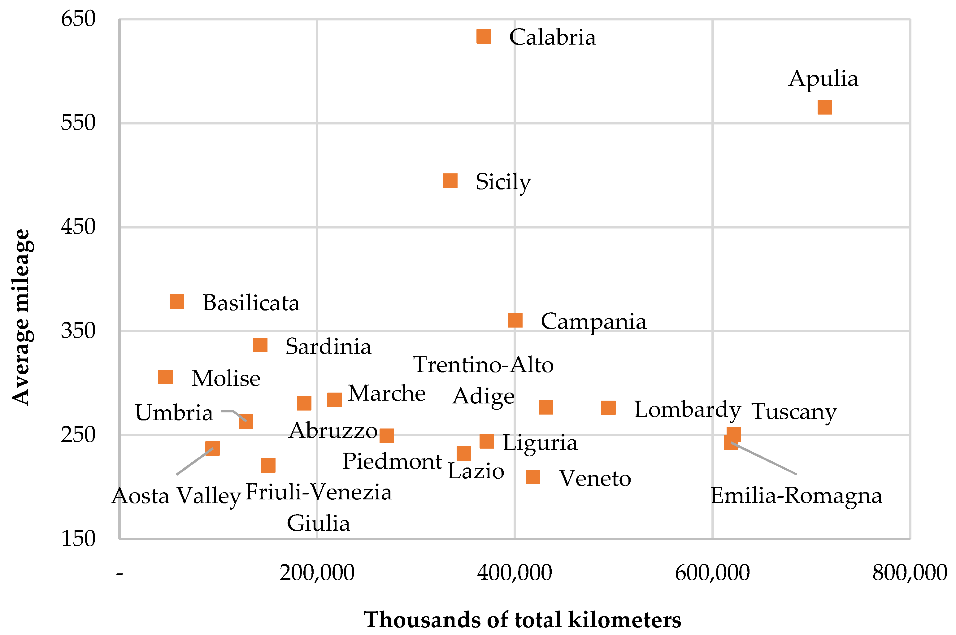
In order to correctly attribute pollutant emissions to trips made by private road vehicles, these were counted only once when several people travelled together. Furthermore, by definition, the main means of transport used was indicated for each trip, i.e., the one with which the greatest distance was covered. This implies that, for those particularly distant destinations, where the greatest distance was covered by other means, such as a plane or train, the possible use of an additional road vehicle was not recorded. However, it is reasonable to assume that these cases did not lead to an excessive underestimation of road journeys. The preponderance of motorized vehicle usage is a consequence of tourists’ choice of destination. Most tourism trips are intra-regional or to regions bordering on the origin of the flows, while localities further away from the place of origin of the trips are reached preferably by other means than the road ones and represent a lower percentage of the total. This was the case, for example, of choosing to reach Sicily by air or Sardinia by waterways. In these cases, once at the destination, the possible use of a road vehicle will be less important in terms of distance travelled than the distance calculated to reach the destination. Therefore, the number of kilometers “lost” compared to the actual kilometers will not be as relevant compared to the overall number of kilometers travelled.
Estimating the distances covered by trips (necessary to estimating emissions) was mainly performed using the distance matrices released by ISTAT. By matching the trip dataset and the distance matrices, using the unique ISTAT code per municipality of origin and destination as keys, it was possible to estimate the distances of 95.6% of the trips, which were subsequently validated using commercial road graph systems (e.g., Google Maps).
The “Database of Average Emission Factors of Road Transport in Italy” was used as a reference to estimate pollutant emissions. This database is used to draft the National Inventory of Atmospheric Emissions, which ISPRA carries out annually as a tool for verifying the commitments undertaken at the international level to protect the atmospheric environment. Specifically, the estimation model used, whose development is coordinated by the European Environment Agency, is the COPERT 5 classification (updated version 5.22). The COPERT 5 classification identifies specific average emission factors, fuel used, vehicle capacity and Euro standard per vehicle category. Therefore, the following correspondence between the vehicle categories of the travel dataset and the COPERT 5 classification was assumed:
  • Cars (aggregating rental cars and own cars/friends) Passenger → Cars
  • Motorhomes, caravans + vans → Light Commercial Vehicles
  • Motorbikes, scooters → Motorcycles
  • Other (truck, lorry, etc.) (This category includes different types of vehicles, so, after some simulations and comparisons with national emissions from the road transport sector, it was decided to attribute 90% of the mileage produced by this category to Light Commercial Vehicles (to which vans would belong), and the remaining 10% to Heavy Duty Trucks) → Heavy Duty Trucks.
For each year, the mileage of trips made with vehicles belonging to the same COPERT 5 vehicle category was aggregated (the mileage of the “Other” category was broken down as indicated before).
The classification of vehicles by fuel used, engine capacity and Euro standard was determined on the assumption that it could be estimated from the composition of the circulating Italian fleet for each reference year (ACI data: http://www.aci.it/laci/studi-e-ricerche/dati-e-statistiche.html accessed on 23 March 2021); the classification, in particular, was constructed with a few approximations—among the most relevant, cars with a capacity of less than 800 cc were considered within the class with an engine capacity of 800–1400 cc; motorbikes were considered from 250 cc; Heavy Duty Trucks with diesel fuel were considered up to a weight of 7.5 tonnes).
For the calculation of pollutant emissions, it was decided to take into account the average COPERT 5 emission factors for the “total” driving cycle, which is an overall measure for the “urban”, “extra-urban” and “motorway” areas.
Therefore, having divided the total mileage travelled in the trips for each reference year, making it compatible with the COPERT 5 classification, and having selected the average emission factors to be used, the emissions produced by each means of transport were estimated for each pollutant present in the “Database of Average Emission Factors for Road Transport in Italy”.
Therefore, by adding up the estimated emissions for each type of vehicle, we finally arrived at an estimate of the total air pollutants produced annually by the road transport sector, linked to Italian tourism activity within the country, over the 2015–2019 study period.
The air pollutants (whose overall composition was considered) selected and analyzed were:
  • carbon monoxide (CO);
  • volatile organic compounds (VOCs);
  • nitrogen oxides (NOx);
  • fine particulate matter (PM2.5);
  • carbon dioxide (CO2).
Ultimately, the mileage travelled and the resulting air emissions were added to the initial dataset of individual trip legs.
In this way, five indicators were produced, one for each atmospheric pollutant considered, representative of the environmental pressure due to road transport for tourism purposes on Italian soil. The emissions of each indicator, expressed in tonnes, were calculated at a national level and comparable over 2015–2019. An estimate of the emissions produced by trips to a specific region in each reference year was also determined. This was done by breaking down the trips each year by region of destination, estimating the emissions using the same procedure as described for the national figure.
In this case, the indicators, still expressed in tonnes, were calculated at the regional level (by breaking down the national figure by region of travel destination), thus acquiring comparability not only in time but also in space. However, interpretation, in this case, could be more complex, as all emissions produced during the trip are attributed to the destination region.

3. Results

3.1. National Analysis

The analysis of the usage of private motor vehicle means of transport identified an increase in the average annual mileage over the period, rising from 268.5 km/trip in 2015 to 303.1 and 293.9 in 2018 and 2019 (Figure 1). The increasing number of trips per year brought a relevant increment in the total annual mileage, which peaked at 7.2 billion km in 2018 from 5.0 in 2015. Table 5 shows that the largest share of mileage was represented by tourists using their car (90.31–94.93), followed by the category “Motorhomes, caravans + vans”, whose contribution seemed to be decidedly lower (3.70–8.40), and finally by two-wheelers and heavier vehicles, whose contribution was found to be marginal.
The estimates of pollutants are shown in Table 6. They varied steadily from year to year but showed similar behavior among them: the starting year recorded the lowest value for all pollutants; in 2016, there was a general growth, followed by a recession in the following year; 2018 was by far the highest year for all emissions; finally, 2019 was probably the year that most characterized the behavior of individual emissions, with some returning to values close to those recorded in the starting year, while others showed a smaller decrease while maintaining their high value. This behavior can be seen in the following graph (Figure 2), where the percentage growth of each pollutant is shown, taking 2015 as the base. Specifically, CO2 was the pollutant with the highest growth in all the years considered, even reaching an increase, in 2018 compared to 2015, of 51.6%, and closing the period with a growth of 27.5%; the pollutants that conversely showed a most modest increase throughout the time interval (except for 2017) were CO and VOCs, which, despite, this showed a growth of 29.5% and 27.8%, respectively, in 2018, with a further increase in 2019 of 5% for CO and 2.6% for VOCs.
The maximum value reached by all pollutants in 2018 could be explained by the following: a peak in emissions from cars, the main vehicle category responsible for the pollutants emitted (especially CO and VOCs, whose car contribution was more than 90% for each year of the study period) (Table 7); and the maximum value also reached by the category “Motorhomes, caravans + vans”, whose major contribution was in the emissions of NOx and PM2.5 (respectively, 16.6% and 24.3% in 2018). The highest value was also reached by the category “Other (lorries, trucks, etc.)”, which, however, played a fairly marginal role overall (the major contribution was in the emissions of NOx, which reached the maximum value of 4.3% in 2018). The difference in pollutants produced between 2017 and 2019 can largely be attributed to the category “Motorhomes, caravans + vans”: the emissions produced by cars were more or less similar (in fact, there was no great difference in CO and VOC levels between the two years), while the values for “Motorhomes, caravans + vans” remained closer to the maximum reached in 2018, thus explaining the high values of NOx and PM2.5 pollutants.

3.2. Regional Analysis

After analyzing the pollutants produced at the national level, the emissions generated by the region of destination of the trips were examined (emissions, as described in the Materials and Methods, were attributed entirely to the region of destination). Consequently, the results were determined by the number of trips collected into the destination region, considering inter-regional and intra-regional flows (Table 8) and the distance covered during a trip in terms of kilometers (Figure 3).
It can be seen from the data that, over the years, a group of regions receiving the largest number of trips was consolidated. These were almost exclusively regions in the central–north area which occupied, albeit in a variable manner over the years, the top positions in the ranking; they were Lombardy, Trentino-Alto Adige/South Tyrol, Veneto, Emilia-Romagna, Tuscany and Lazio, plus a single region in the south, Campania, and, since 2016, also Liguria, Puglia and Piedmont.
However, the average mileage travelled per trip was higher for trips to the south (Campania, Basilicata, Calabria and Apulia) and islands (Sicily and Sardinia) (Figure 3). As for 2019, the region to which trips produced the highest level of emissions was Apulia, followed by Tuscany and Emilia-Romagna; conversely, the regions to which trips produced fewer emissions were Molise, Basilicata and Valle d’Aosta (which were also the regions to which the fewest trips were made).
Table 9 shows the emissions in tonnes by destination region in 2019: Puglia, Tuscany and Emilia-Romagna were the regions to which journeys produced the most emissions for all pollutants; the three regions to which journeys produced the least emissions were Molise, Basilicata and Valle d’Aosta, respectively.
Finally, Table 10 shows the percentage variation of pollutants by region of destination between the first and last year of the reference period.
An initial examination showed that the percentage variations were mainly positive. Specifically, the region that showed the greatest positive variation was Sicily, with significant growth in all emissions above 350%, even reaching a peak of 475.8% for CO2; the region, however, that recorded the most pronounced negative variation was Umbria, with pollutants displaying an overall decrease between 35% and 50%.

4. Discussion

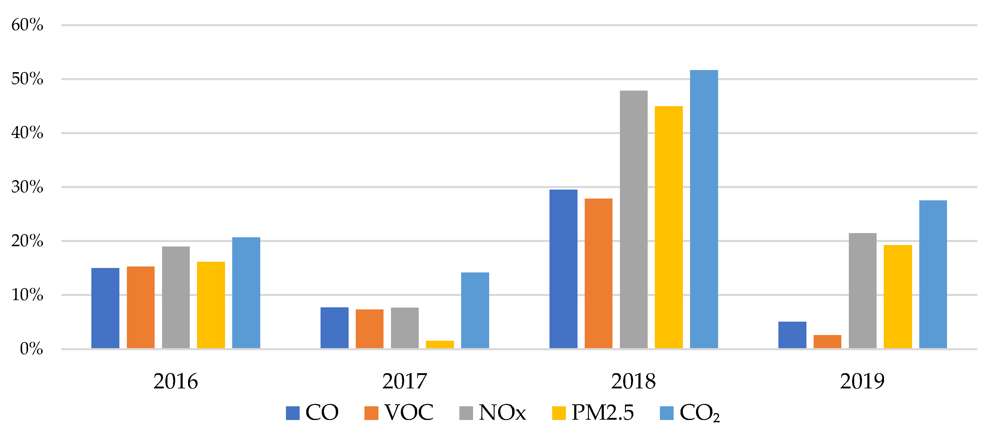
The comparison of the estimated emissions caused by the domestic trips concerning tourism activity examined in this work with the total emissions caused by the road transport in Italy, estimated by ISPRA using the same COPERT 5 classification [31], raises some interesting points. The total road transport emissions include the emissions produced by all types of vehicles included the category “buses”, which was excluded from the tourism analysis; in addition, the mileage produced by Light Commercial Vehicles and Heavy Duty Trucks was correctly attributed. Consequently, for each year of the time interval 2015–2019, the percentage of estimated emissions out of the total road transport emissions could be evaluated considering every pollutant examined in the work (Table 11). The percentages computed are not so high (around 1–3%), but neither so irrelevant if we consider the restricted field of analysis. According to the trend of estimated emissions, the minimum value of pollutants was reached in 2015 and the highest in 2018. The more consistent contribution was due to CO and VOCs, which seemed to show an analogous trend. The other pollutants, NOx, PM2.5 and CO2, were slightly more heterogeneous (especially in 2018 and 2019), with smaller percentages than CO and VOCs.
In Table 12, it is noted that the percentages of pollutants attributable to cars used for tourism are higher than those of the total in Table 11. Therefore, policies that discourage the use of private cars for tourism purposes would be desirable, as they would mitigate current attributable emission levels.
A comparison of studies published in the literature is not simple, nor is the purpose of this paper. Different types of methods are used to estimate emissions from tourism activity and its transport, obtaining variable results [32]. One of the most common ways to account for tourism emissions, as noted in the Introduction, is the tourism Satellite Account (TSA). The TSA is an internationally accepted framework developed by the UNWTO in collaboration with other organizations’ actions to measure the impact of tourism on the national economy. The TSA is based on the estimate of the expenditure of tourists for products and services; consequently, these expenditures translate into the contribution of tourism to added value and employment. Some studies have estimated tourism emissions based on TSA, assuming that the same share contributes to the added value of the economic system and that employment can be used to determine its share of emissions of GHGs or other pollutants from a production point of view, e.g., [33,34]. Our study sought to move beyond the purely economic approach of the TSA, offering a “new” environmental indicator relating to atmospheric emissions related to tourism travel and, in particular, only to those trips made using road transport. Our work has a well-defined “tourism–environmental” perimeter but was addressed using only data from official national statistics; therefore, it will increase the official information offered on these issues, which is unfortunately still sparse due to a lack of suitable basic data.
As a general consideration, in fact, this work further highlights the need for measurement, reporting and verification systems across all tourism value chains, such as the relationship between tourism and the environment.
The attempt presented here exploits basic data from official Italian statistical sources but collected for priority purposes other than “tourism and the environment”.
Therefore, basic data are needed, at least at a European level, which is essential to then define useful indicators for monitoring the various components of tourism sustainability, or even the environmental and social dimensions that are not currently considered by official European statistics.
The basic data, common to all European countries to monitor the relationship between tourism and the environment, become fundamental if one really wishes to strive towards sustainable and environmentally friendly tourism.

5. Conclusions

When travelling for tourism, several factors determine the choice of the main means of transport to reach the destination: the distance from the region of origin, the presence of airport or railway infrastructures, the cheapness of the means of transport, the number and composition of the group of people leaving together and, last but not least, the versatility that the means of transport offers, allowing different degrees of flexibility in moving to the destination [35]. Based on these considerations, most residents prefer the car as their main means of transport, chosen for more than 7 out of 10 personal trips made in Italy and, among all private road means of transport, for 9 out of 10 trips.
However, the car is also the vehicle that contributes the most to all pollutant emissions, with values ranging, in the most recent year analyzed here, 2019, between 70.8% of PM2.5 and 94.9% of VOCs. Compared to other means of road transport, the most significant contribution to air pollutants comes from the use of camper vans, caravans and vans, which mainly influence emissions of PM2.5 (26.2%) and NOx (18.6%).
The analysis showed that emissions vary steadily from year to year but that their behavior is similar. For all kinds of pollutants, 2018, when the flow of tourism trips was the most consistent during the period under review, was by far the year with the highest amount of tonnes emitted.
The regional analysis carried out limited the emission contribution of road trips to the destination regions only; in order to refine and therefore increase the precision of the territorial attribution of pollutants, as future development, a more laborious breakdown of the trip into regional sections is hypothesized, to which the pollutant emissions of the route between the origin and destination of the trip can be attributed.
Moreover, the analysis will be enriched with new content when, in addition to trips with an overnight stay, same-day visits are included, which, given their nature, are carried out mainly by car, towards destinations close to those of origin, characterizing this part of tourism as intra-regional proximity tourism even more than trips.
The results achieved so far on the temporal and spatial distribution of the principal atmospheric emissions due to road-transport-related to domestic trips for tourism purposes have only been possible thanks to the exploitation, through an integrated analysis, of several sources of official statistics. The challenge of the present work is to contribute in monitoring a part of the tourism–environment issue, without referring to accounting schemes, but instead by using both an official sample survey on tourism—which is under European Regulation—and the environmental monitoring data from the national inventory of atmospheric emissions. The latter is the main national reference in the “environmental” areas, to meet the main reporting obligations envisaged in the international context, such as those provided for by the United Nations Framework Convention on Climate Change (UNFCCC), the Kyoto Protocol, the European Union Greenhouse Gas Monitoring Mechanism and the Convention on Long-Range Transboundary Pollution (CRLTAP/UNECE), as well as the related protocols for the reduction of emissions of various substances.
This issue, strongly supported by the European Union, is part of the 2030 Agenda for Sustainable Development, signed by the governments of 193 UN member countries in 2015, including Italy, within which three of the seventeen SDGs refer to tourism (Targets 8.9, 12.b and 14.7 in particular and Goal 13 in general) [36]. One of the statistical measures that is helpful in monitoring the Sustainable Development Goals of Target 12.b is the percentage composition of trips made by residents in the national territory by the main means of transport. Since 2018, these data, coming from the “Trips and Holidays” survey carried out by ISTAT, are regularly transmitted on an annual basis and, together with other data, contribute annually to the National Report on the SDGs [37], which describes Italy’s position along the path of sustainable development.
The indicators produced by this work could enrich the wealth of information on measures taken to monitor the SDGs in the tourism sector, which is recognized not only as an important sector for inclusive economic growth aimed at local communities but also as a potential accelerator towards sustainability, through the adoption of sustainable models of consumption and production.
In the immediate future, moreover, these analyses will enrich the ISPRA core set of indicators [38] on the environment–tourism theme in a stable manner. However, they will also be the starting point for further joint analyses between the two institutes to expand the information available to them, as well as representing new useful tools for researchers engaged in monitoring sustainable tourism in general and the tourism–environment relationship in particular.
The major limitations of this work also represent the potential for future research on this topic and sustainable tourism in particular. The current availability of data does not allow, at the moment, for an exhaustive assessment of the impact of two of the main drivers of change on the environmental sustainability of tourism: the impact of demographic and socio-economic change of population—such as the ageing of western societies—and ecological transition.
For instance, we can pose some very basic questions whose answers can design different futures for tourism habits: are the choices of the means of transportation and of the tourism destinations age-dependent or connected to the tourists’ level of wealth/income (e.g., do “young/old” or “rich/poor” tourists prefer different destinations?)? Is the wealth level of the tourist destination or the quality of its infrastructure network correlated to the type of tourists visiting that destination (e.g., if the railroad network of the destination region is not well-developed, do the tourists prefer to reach it by car?)? Does the mean of transportation choice depend on the family composition (e.g., do larger families with underaged children prefer to use private cars?)? Will the ecological transition reduce the polluting emissions of some means of transportation more than others? If we can answer these questions affirmatively, which we believe is possible, we will be able to begin a relevant debate on the perspectives of sustainable tourism, developing adequate policies and infrastructure development solutions. In short, a numerous series of insights and research ideas linked to socio-economic and geographical factors, which encourage tourists to use the car as the main means of transport for tourism purposes, could be studied in depth if the data on these topics already available were enriched and combined.

Author Contributions

Conceptualization, G.F. and B.D.; methodology, L.B.; B.D. and G.F.; validation, E.d.B. and S.I.; data curation, L.B.; B.D. and G.F.; writing—original draft preparation, L.B.; B.D.; E.d.B.; G.F. and S.I. All authors have read and agreed to the published version of the manuscript.

Funding

This research received no external funding.

Institutional Review Board Statement

Not applicable.

Informed Consent Statement

Not applicable.

Data Availability Statement

Not applicable.

Acknowledgments

Antonella Bernetti and Riccardo De Lauretis (Air Emission Inventory Unit of ISPRA).

Conflicts of Interest

The authors declare no conflict of interest.

Appendix A. Weighting Procedure and Accuracy of the Estimates in the “Trips and Holiday” Survey

Each estimation method is based on the principle that the subset of the units of the population included in the sample must also represent the complementary subset consisting of the remaining units of the population. This principle is generally achieved by assigning to each unit included in the sample a weight that can be seen as the number of population elements represented by that unit. The “Trips and Holidays survey” is a module embedded into the “Household Budget Survey” (HBS) carried out by ISTAT. It is a large-scale survey conducted monthly with the CAPI (Computer-Assisted Personal Interview) technique, over a theoretical yearly sample of 28,000 households in 2015/2016 and 19,500 households from 2017 to 2019. The reduction of the theoretical sample size has been possible due to a new strategy of collecting interviews in accordance with the company in charge of the data collection, which led to an increase in the efficiency in this phase. The sampling design is partly single-stage and partly two-stage, with stratification of primary sampling units. It aims to provide a large number of estimates of population parameters, such as counts, totals, proportions, averages, etc. The estimation of the population parameters for HBS has been done with methods based on the direct approach using values of the variable of interest observed on the sample units belonging to the domain of interest. These are the standard methods used by ISTAT. In general, for the estimation of a total, the following two operations are performed:
  • computation of the weight to be assigned to each unit included in the sample;
  • calculation of the estimates as weighted sums of the target variables’ values using weights determined in Step 1.
The weight given to each unit is obtained according to a procedure divided into several steps:
  • the starting weight of each sample unit, named the direct weight, is calculated according to the sampling design, as the reciprocal of the inclusion probability;
  • the starting weight is adjusted to account for non-response, obtaining the base weight;
  • correction factors of the base weight basis are computed to take into account equality constraints between some known parameters of the population and the corresponding sample estimates;
  • the final weight is obtained as the product between the base weight and the correction factors.
The class of estimators corresponding to the operations described above and adapted for HBS is known as calibration estimators (Deville, Särndal 1992), since both the adjustment to correct for non-response and the weight correction to achieve consistency with known population parameters are obtained by solving a constrained minimization problem. In detail, we wish to minimize the distance between the weights before and after the calibration phase. Calibration estimators need to satsify:
  • efficiency criteria in terms of sample variance and bias due to the presence of total and partial non-responses and frame undercoverage.
  • external and internal coherence. The external consistency of the estimates arises whenever known totals are available from external sources. Estimates of the total produced by the survey should generally match or not deviate excessively from the known values of these totals. The internal consistency of the estimates is achieved when all the estimates of the same aggregate coincide with each other. This result can be obtained using a unique system of weights.
  • Calibration estimators were chosen as:
  • they yield, generally, more efficient estimates than those obtained using direct estimators; the higher the correlation between the auxiliary variables and the target variables, the greater the efficiency;
  • they are approximately unbiased designs;
  • they produce estimates of totals that coincide with the known values of these totals;
  • they mitigate the non-response bias effect;
  • they reduce the bias due to the undercoverage of the frame from which the sample is selected.
  • Accuracy of the Estimates
For the evaluation of the sampling errors of the estimates, ISTAT usually uses approximated variance estimation methods. In fact, for most of the estimation procedure, an analytical expression of the estimator variance is not available since:
  • ISTAT surveys are carried out using complex sampling designs, generally based on multiple selection stages, on the stratification of the units and without a repetition selection scheme, with varying selection probabilities among units;
  • estimates are determined using calibration estimators, which are non-linear functions of the sample information.
The estimation methods of the sample variance generally used in ISTAT, and particularly for HBS, are based on the method of linearization of Woodruff (1971), which estimates the sample variance in the case where the estimators used are non-linear functions of the sample data.
ISTAT implements these variance estimation methods in the generalized software ReGenesees, which features a user-friendly interface and is currently used to estimate the sampling errors of the estimates produced by ISTAT surveys, HBS included. In addition, this software makes it possible to compute important analysis statistics, which provide valuable tools to evaluate the adopted sampling design. In particular, it is possible to evaluate:
  • the overall efficiency of the sampling design;
  • the impact on the efficiency of the estimates due to stratification, the number and type of selection stages and weighting effect.
By this method, the sampling error may be expressed in terms of absolute error (standard error) or relative error.
Since each estimate corresponds to a sampling error, to allow correct use of the information produced by the survey, it would be necessary to publish the corresponding sampling error for each estimate. To overcome this calculation but having, at the same time, an assessment of the sample variability of all the estimates of interest, a generalized variance error representation is also provided. This is a summary obtained using regression models that relate the estimates to the corresponding sampling errors.
However, the problem is rather complex for the estimates of totals of quantitative variables, such as those of the “Trips and Holidays” survey, because an adequate theoretical basis for the interpolation of the sample errors of the estimates has not yet been devised. Therefore, the approach adopted to deal with the case of quantitative variables is empirical, and it is based on the experimental evidence that the absolute error of a total estimate is an increasing function of the total itself.
The model used for estimates of total trips, referring to the generic domain d, is as follows:
σ ^ ( Y ^ d ) = a + b Y ^ d + c Y ^ d 2
where the parameters a, b and c are estimated by using the method of least squares and adapting model (A1) to a cloud of points made by a consistent number of couples of values ( σ ^ ( Y ^ d ) , Y ^ d ) , which represent the absolute sample error of an estimate and the estimated point, respectively. In consideration of the fact that model (A1) is empirical, the group of estimates Y ^ d used for the interpolation of the model has been determined by including the principal estimates that are disseminated.
In order to obtain a better fit to the point cloud, a model was interpolated—with reference to the quarters and/or the entire year, depending on the territorial domain—for each of the following subgroups of estimates:
  • number of nights for business trips;
  • number of nights for personal trips;
  • total number of nights;
  • number of business trips;
  • number of personal trips;
  • total number of trips.
Circumscribing to the content of this paper, the calculation of the a, b and c coefficients and the R2 (coefficient of determination) of the models used for the interpolation of sample errors of trips is presented in Table A1. They refer to the years 2015 to 2019. By using these, the calculation of relative errors for the estimates of all numbers presented in this paper is possible. To help the users, referring to the principal estimates presented in Table 1 of the paper, the relative errors are presented in Table A1. Starting from these estimates and the relative errors, it is possible to build the confidence interval, which, with a predetermined level of confidence, contains within it the true, but unknown, value of the parameter being estimated. The confidence interval is calculated by adding and subtracting from the point estimate its absolute sampling error, multiplied by a coefficient k that depends on the level of confidence P; considering the traditional confidence level of P = 95%, the corresponding coefficient k is equal to 1.96. With reference to a generic estimate, this interval takes the following form: { Y ^ k σ ^ ( Y ^ ) , Y ^ + k σ ^ ( Y ^ ) } An example of a confidence interval can be found in Table A2.
Using the estimated values of the model parameters (A1) and dividing both sides of the model by the value of the estimate Y ^ d , we arrive at the following second-degree equation:
a + [ b ε ( Y ^ d ) ] Y ^ d + c ( Y ^ d ) 2 = 0
whose positive root is expressed by the following formula:
Y ^ d = [ b ε ( Y ^ d ) ] [ b ε ( Y ^ d ) ] 2 4 a c 2 c
Table A1. Point estimates of domestic trips (thousands), relative errors ε, coefficients of the model and R2. Years 2015–2019.
Point Estimate
(Number)
Relative Error abcR2
2015
Total trips47,0930.048191,012.5390.072243506−0.00000000060.96
Personal trips41,7360.052190,113.1300.077697273−0.00000000070.96
Business trips53560.12141,066.3620.198324651−0.00000001590.96
2016
Total trips54,7140.043205,773.7320.065059358−0.00000000050.96
Personal trips49,5960.049194,439.6310.075567529−0.00000000060.96
Business trips51180.10543,720.2570.160974363−0.00000001260.95
2017
Total trips53,6470.036197,878.7550.051595448−0.00000000040.96
Personal trips49,4290.041183,440.9300.060093384−0.00000000050.96
Business trips42180.10233,748.1850.154587543−0.00000001440.97
2018
Total trips62,8610.032211,734.7410.045162113−0.00000000030.95
Personal trips56,3530.036196,478.6450.052828719−0.00000000040.95
Business trips65080.08542,909.9320.123041320−0.00000000690.97
2019
Total trips54,2530.033184,929,6610.046704815−0.00000000030.96
Personal trips48,4100.038174,507,3600.054015643−0.00000000040.97
Business trips58430.08143,257,7190.120873896−0.00000000810.96
Source: ISTAT, Trips and Holidays Survey.
Table A2. Example of calculation of interval confidence (P = 0.95, k = 1.96). Year 2016.
Point estimate54,714
Relative error ε0.043
Interval Estimates
Half width of the interval(54,714 × 0.043) × 1.96 = 4611
Lower confidence limit54,714 − 4611 = 50,103
Upper confidence limit54,714 + 4611 = 59,325
Source: ISTAT, Trips and Holidays Survey.

References

  1. UNEP and UNWTO. Making Tourism More Sustainable—A Guide for Policy Makers; UNEP and UNWTO: Paris, France, 2005. [Google Scholar]
  2. Sustainable Tourism for Development Guidebook–Enhancing Capacities for Sustainable Tourism for Development in Developing Countries. 2013. Available online: https://www.e-unwto.org/doi/epdf/10.18111/9789284415496 (accessed on 22 October 2021).
  3. United Nation World Tourism Organization. Recommendations for the Transition to a Green Travel and Tourism Economy; UNWTO: Madrid, Spain, 2021. [Google Scholar] [CrossRef]
  4. Eurostat. Tourism Database. Available online: https://ec.europa.eu/eurostat/web/tourism/data/database and https://ec.europa.eu/eurostat/web/tourism/data/main-tables (accessed on 19 August 2021).
  5. European Parliament. Research for Tran Committee—From Responsible Best Practices to Sustainable Tourism Development. 2016. Available online: https://www.europarl.europa.eu/RegData/etudes/STUD/2015/573421/IPOL_STU(2015)573421_EN.pdf (accessed on 20 August 2021).
  6. ETC/ULS. Tourism and the Environment towards a Reporting Mechanism in Europe, Report. 2018. Available online: https://www.eionet.europa.eu/etcs/etc-uls/products/etc-uls-report-01-2018-tourism-and-the-environment-towards-a-reporting-mechanism-in-europe (accessed on 20 August 2021).
  7. UNWTO (United Nation World Tourism Organization). Transforming Tourism for Climate Action. Available online: https://www.unwto.org/sustainable-development/climate-action (accessed on 3 November 2021).
  8. World Tourism Organization and International Transport Forum. Transport-Related CO2 Emissions of the Tourism Sector–Modelling Results; UNWTO: Madrid, Spain, 2019. [Google Scholar] [CrossRef]
  9. UNFCC. UN Climate Change Conference–December 2019. Available online: https://unfccc.int/cop25 (accessed on 3 November 2021).
  10. One Planet Sustainable Tourism Programme—One Planet Vision for a Responsible Recovery of the Tourism Sector. 2020. Available online: https://webunwto.s3.eu-west-1.amazonaws.com/s3fs-public/2020-06/one-planet-vision-responsible-recovery-of-the-tourism-sector.pdf (accessed on 3 November 2021).
  11. The Glasgow Declaration. Available online: https://www.oneplanetnetwork.org/programmes/sustainable-tourism/glasgow-declaration (accessed on 28 September 2021).
  12. Eurostat, Tourism Satellite Accounts in the European Union Volume 1–4, Statistical Working Papers Luxembourg: Office for Official Publications of the European Communities. 2010. Available online: https://ec.europa.eu/eurostat/web/main/search?p_p_id=estatsearchportlet_WAR_estatsearchportlet_INSTANCE_bHVzuvn1SZ8J&p_p_lifecycle=1&p_p_state=maximized&p_p_mode=view&_estatsearchportlet_WAR_estatsearchportlet_INSTANCE_bHVzuvn1SZ8J_action=search&_estatsearchportlet_WAR_estatsearchportlet_INSTANCE_bHVzuvn1SZ8J_pageSize=11&_estatsearchportlet_WAR_estatsearchportlet_INSTANCE_bHVzuvn1SZ8J_theme=PER_INDCOM&_estatsearchportlet_WAR_estatsearchportlet_INSTANCE_bHVzuvn1SZ8J_sort=lastUpdateDate&_estatsearchportlet_WAR_estatsearchportlet_INSTANCE_bHVzuvn1SZ8J_collection=CAT_METWP&p_auth=BbU3Y2Lr&_estatsearchportlet_WAR_estatsearchportlet_INSTANCE_bHVzuvn1SZ8J_publicationDate=2010 (accessed on 28 September 2021).
  13. ISTAT. Integrated Economic and Environmental Accounts for Tourism. Available online: https://www.istat.it/en/archivio/228239 (accessed on 30 August 2021).
  14. Regulation (EU) No 692/2011 of the European Parliament and of the Council of the 6th of July 2011 Concerning European Statistics on Tourism and Repealing Council Directive 95/57/EC. Available online: https://eur-lex.europa.eu/LexUriServ/LexUriServ.do?uri=OJ:L:2011:192:0017:0032:EN:PDF (accessed on 19 August 2021).
  15. UNECE. Convention on Long Range Transboundary Air Pollution (CLRTAP). Available online: https://unece.org/convention-and-its-achievements (accessed on 23 April 2021).
  16. Convention United Nations Framework on Climate Change (UNFCCC). Available online: https://unfccc.int/process-and-meetings/the-convention/what-is-the-united-nations-framework-convention-on-climate-change (accessed on 23 April 2021).
  17. IPCC (Intergovernmental Panel on Climate Change). Special Report on Global Warming of 1.5 °C. Available online: http://www.ipcc.ch/report/sr15/ (accessed on 20 August 2021).
  18. Gössling, S.; Higham, J. The Low-Carbon Imperative: Destination Management under Urgent Climate Change. J. Travel Res. 2021, 60, 1167–1179. [Google Scholar] [CrossRef]
  19. Stern Review: The Economics of Climate Change. Available online: http://mudancasclimaticas.cptec.inpe.br/~rmclima/pdfs/destaques/sternreview_report_complete.pdf (accessed on 20 August 2021).
  20. Higham, J.; Ellis, E.; Maclaurin, J. Tourist Aviation Emissions: A Problem of Collective Action. J. Travel Res. 2018, 58, 535–548. [Google Scholar] [CrossRef]
  21. Scott, D.; Hall, C.M.; Gössling, S. Global tourism vulnerability to climate change. Ann. Tour. Res. 2019, 77, 49–61. [Google Scholar] [CrossRef]
  22. Larsson, J.; Elofsson, A.; Sterner, T.; Åkerman, J. International and National Climate Policies for Aviation: A Review. Clim. Policy 2019, 19, 787–799. [Google Scholar] [CrossRef] [Green Version]
  23. Peeters, P.; Higham, J.; Kutzner, D.; Cohen, S.; Gössling, S. Are technology myths stalling aviation climate policy? Transp. Res. Part D Transp. Environ. 2016, 44, 30–42. [Google Scholar] [CrossRef] [Green Version]
  24. Scott, D.; Hall, C.M.; Gössling, S. A report on the Paris Climate Change Agreement and its implications for tourism: Why we will always have Paris. J. Sustain. Tour. 2016, 24, 933–948. [Google Scholar] [CrossRef]
  25. Research for TRAN Committee–Overtourism: Impact and Possible Policy Responses. Prepared for the European Parliament; 2018. Available online: http://www.europarl.europa.eu/RegData/etudes/STUD/2018/629184/IPOL_STU(2018)629184_EN.pdf (accessed on 20 August 2021).
  26. ISTAT. La Nuova Indagine Sulla Domanda Turistica. Available online: https://www.istat.it/it/archivio/222043 (accessed on 29 July 2021).
  27. UNWTO (United Nation World Tourism Organization). International Recommendations on Tourism Statistics 2008 (IRTS 2008), ST/ESA/STAT/SER.M/83/Rev.1, Madrid and New York. 2010. Available online: https://unstats.un.org/unsd/publication/Seriesm/SeriesM_83rev1e.pdf (accessed on 19 August 2021).
  28. Eurostat. Methodological Manual for Tourism Statistics–Version 3.1. Available online: http://ec.europa.eu/eurostat/web/products-manuals-and-guidelines/-/KS-GQ-14-013 (accessed on 29 July 2021).
  29. ISTAT. Trip and Holidays: Microdati ù. Available online: https://www.istat.it/en/archivio/178698 (accessed on 29 July 2021).
  30. Deville, J.-C.; Sarndal, C.-E. Calibration Estimators in Survey Sampling. J. Am. Stat. Assoc. 1992, 87, 376. [Google Scholar] [CrossRef]
  31. ISPRA. Serie Storiche Emissioni–Dati Trasporto Stradale 1990–2019. Available online: http://www.sinanet.isprambiente.it/it/sia-ispra/serie-storiche-emissioni/dati-trasporto-stradale/view (accessed on 30 August 2021).
  32. Henrik, G.; Susana, L. The who, why and where of Norway’s emissions from tourist travel. Environ. Adv. 2021, 5. [Google Scholar] [CrossRef]
  33. Perch-Nielsen, S.; Sesartic, A.; Stucki, M. The greenhouse gas intensity of the tourism sector: The case of Switzerland. Environ. Sci. Policy 2010, 13, 131–140. [Google Scholar] [CrossRef]
  34. Russo, M.; Relvas, H.; Gama, C.; Lopes, M.; Borrego, C.; Rodrigues, V.; Robaina, M.; Madaleno, M.; Carneiro, M.; Eus´ebio, C.; et al. Estimating emissions from tourism activities. Atmos. Environ. 2020, 220. [Google Scholar] [CrossRef]
  35. Sabato, M.; Dattilo, B.; Di Torrice, M. Destinazione Italia: Turismo e Competitivita’ Territoriale. Un’analisi Regionale della Domanda Turistica dei Residenti. XL Annual Scientific Conference of A. I. S. Re. (Associazione Italiana di Scienze Regionali), L’Aquila, Italy. 2019. Available online: https://www.aisre.it/images/aisre/2019_papers/Sabato-16-16-Sabato-Mariangela.pdf (accessed on 18 August 2021).
  36. United Nations. Transforming Our World: The 2030 Agenda for Sustainable Development. Available online: https://epale.ec.europa.eu/sites/default/files/21252030_agenda_for_sustainable_development_web.pdf (accessed on 29 July 2021).
  37. ISTAT. The SDGs Report. Available online: https://www.istat.it/en/well-being-and-sustainability/sustainable-development-goals/sdgs-report (accessed on 29 July 2021).
  38. ISPRA. Annuario dei dati Ambientali. Available online: https://annuario.isprambiente.it/ (accessed on 10 November 2021).
Figure 1. Kilometers travelled (in thousands) and average mileage (in km/trip) of trips in Italy (2015–2019). Source: ISPRA elaboration on ISTAT data.
Sustainability 13 12712 g001
Figure 2. Percentage growth of each pollutant’s emissions, taking 2015 as base year. Source: ISPRA.
Sustainability 13 12712 g002
Figure 3. Kilometers travelled and average mileage to travel to the region of destination (2019). Source: ISPRA elaboration on ISTAT data.
Sustainability 13 12712 g003
Table 1. Domestic trips by the main purpose of the trip. Years 2015–2019, values in thousands. Percentage compositions are also shown.
YearPersonalBusinessTotal Trips
Number%Number%Number%
201541,73688.6535611.447,093100
201649,59690.651189.454,714100
201749,42992.142187.953,647100
201856,35389.6650810.462,861100
201948,41089.2584310.854,253100
Average 2015–201949,10590.154099.954,514100
Source: ISTAT, Trips and Holidays Survey.
Table 2. Domestic trips by main means of transport. Years 2015–2019, percentage compositions.
YearAirTrainWaterwayPrivate Vehicles
Motorized
Coach/Bus
20156.715.21.172.24.8
20165.412.02.376.83.5
20178.511.81.872.55.4
20187.412.32.774.03.6
20197.312.51.772.95.8
Average 2015–20197.112.72.073.74.6
Source: ISTAT, Trips and Holidays Survey.
Table 3. Trips in Italy by type of trip and type of transport. Average years 2015–2019, percentage compositions.
Means of TransportPersonalBusinessTotal Trips
Private motorised vehicles76.152.573.7
Train11.027.812.7
Air6.413.27.1
Coach/Bus4.64.64.6
Waterway2.01.92.0
Total100.0100.0100.0
Source: ISTAT, Trips and Holidays Survey.
Table 4. Domestic trips by type of private motorized transport. Years 2015–2019, percentage compositions.
YearRental CarsPrivate CarsMotorhomes, CaravansMotorbikes, ScootersOthers *
20151.492.13.50.72.3
20161.193.62.00.62.8
20171.294.82.10.61.4
20182.891.22.90.82.3
20191.891.24.00.52.5
Note: * Includes mainly other motor vehicles, such as vans, trucks, lorries. Source: ISTAT, Trips and Holidays Survey.
Table 5. Percentage of mileage travelled by vehicle type, Years 2015–2019.
Type of Vehicle20152016201720182019
Car91.5692.6494.9390.7390.31
Motorhomes/caravans, vans6.605.933.707.918.60
Motorbikes, scooters1.350.951.110.710.67
Other (truck, lorry, etc.)0.490.480.260.640.42
Total100.0100.0100.0100.0100.0
Source: ISPRA.
Table 6. Estimated national emissions in tonnes, Years 2015–2019.
Pollutants20152016201720182019
CO9394.110,800.410,114.812,166.29866.8
VOCs2776.73200.02978.83549.22848.3
NOx2725.13241.12932.34028.03309.2
PM2.5166.9193.8169.4241.9199.0
CO2879,723.01,061,285.41,004,371.31,334,109.81,121,807.0
Source: ISPRA.
Table 7. Emissions from travel in Italy by type of vehicle used. Years 2015–2019. Data in tonnes and percentage compositions.
YearType of VehicleCOVOCsNOxPM2.5CO2
2015Cars8506.1 90.5%2613.994.1%2263.883.1%124.774.8%779,19888.6%
Motorhomes, caravans and vans317.23.4%51.41.9%362.113.3%3621.6%83,674.49.5%
Motorbikes, scooters542.45.8%96.33.5%110.4%1.20.7%8020.40.9%
More28.30.3%15.10.5%88.33.2%4.92.9%8830.11.0%
Total9394.1100%2776.7100%2725.1100%166.9100%879,723100%
2016Cars9984.892,4%3047.995.2%2729.584.2%149.277%952,918.289.8%
Motorhomes, caravans and vans329.63.1%53.41.7%397.812.3%37.819.5%91,035.68.6%
Motorbikes, scooters452.44.2%80.92.5%9.20.3%10.5%6842.40.6%
More33.60.3%17.80.6%104.63.2%5.83%10,489.21.0%
Total10,800.4100%3200100%3241.1100%193.8100%1,061,285.4100%
2017Cars940793%2848.895.6%2627.489.6%143.284.5%936,615.493.3%
Motorhomes, caravans and vans193.21.9%31.31.1%240.68.2%22.213.1%54,5855.4%
Motorbikes, scooters497.24.9%89.53%10.20.3%1.10.6%7719.20.8%
More17.40.2%9.20.3%54.21.8%31.8%5451.70.5%
Total10,114.8100%2978.8100%2932.3100%169.4100%1,004,371.3100%
2018Cars11,201.892.1%336594.8%3178.878.9%172.871.4%1,158,05986.8%
Motorhomes, caravans and vans505.14.2%822.3%669.216.6%58.724.3%152,289.911.4%
Motorbikes, scooters404.43.3%73.32.1%8.30.2%0.90.4%6455.20.5%
More54.90.5%290.8%171.74.3%9.53.9%17,305.81.3%
Total12,166.2100%3549.2100%4028100%241.9100%1,334,109.8100%
2019Cars9080.392%2703.494.9%2592.578.3%140.870.8%967,131.686.2%
Motorhomes, caravans and vans447.54.5%72.62.5%614.518.6%52.126.2%139,928.512.5%
Motorbikes, scooters308.33.1%56.32.0%6.40.2%0.70.4%5062.80.5%
More30.60.3%16.20.6%95.82.9%5.32.7%96840.9%
Total9866.8100%2848.3100%3309.2100%199100%1,121,807100%
Source: ISPRA.
Table 8. Domestic trips made by private motorized means of transport by region of destination. Years 2015–2019, percentage compositions.
Region of DestinationYear
20152016201720182019
Piedmont 3.16.44.24.35.0
Valle d’Aosta/Vallée d’Aoste0.60.70.91.91.8
Lombardy10.49.67.99.58.2
Trentino-Alto-Adige/South Tyrol6.97.78.46.77.1
Veneto11.510.79.99.69.1
Friuli-Venezia Giulia2.03.00.92.43.1
Liguria4.16.67.26.77.0
Emilia-Romagna13.812.910.710.711.7
Tuscany9.010.714.113.611.3
Umbria2.93.13.12.12.2
Marche3.92.52.63.03.5
Lazio9.57.85.47.26.9
Abruzzo3.52.23.92.83.0
Molise0.90.40.20.30.7
Campania6.25.15.95.15.1
Apulia4.65.06.36.95.8
Basilicata0.90.40.80.70.7
Calabria2.61.92.12.52.7
Sicily1.22.52.92.33.1
Sardinia2.30.92.71.71.9
Total100.0100.0100.0100.0100.0
Source: ISTAT, Trips and Holidays Survey.
Table 9. Emissions in tonnes by region of destination (2019).
Region of DestinationCOVOCsNOxPM2.5CO2
Piedmont396.5115.2154.99.648,824.4
Valle d’Aosta/Vallée d’Aoste132.837.355.63.717,493.4
Lombardy739.8216.1264.015.987,207.5
Trentino-Alto Adige/South Tyrol 645.4187.2225.113.775,976.6
Veneto643.6190.3201.111.471,368.5
Friuli-Venezia Giulia209.859.899.96.528,591.1
Liguria545.8155.7204.613.066,892.3
Emilia-Romagna968.7279.9310.018.3106,957.1
Tuscany978.7282.1306.818.1107,049.4
Umbria244.364.464.33.921,982.3
Brands363.799.6111.26.938,049.5
Lazio529.5156.0176.610.360,365.8
Abruzzo347.193.987.95.131,470.5
Molise73.221.821.11.27824.2
Campania635.1186.8184.410.267,358.4
Apulia1089.6320.9348.220.1122,444.4
Basilicata91.327.226.11.49727.5
Calabria529.3151.2213.013.767,343.2
Sicily485.1138.8186.211.960,512.3
Sardinia217.664.068.44.024,368.4
Italy9866.82848.33309.21991,121,807
Source: ISPRA.
Table 10. Percentage change from 2015 to 2019 in emissions by region of destination.
Region of DestinationCOVOCsNOxPM2.5CO2
Piedmont85.385.4100.083.7117.3
Valle d’Aosta/Vallée d’Aoste 164.1174.8125.684.1156.5
Lombardy−6.5−7.512.38.915.8
Trentino-Alto Adige/South Tyrol−9.9−13.94.35.28.6
Veneto−14.6−17.2−7.7−10.2−0.7
Friuli-Venezia Giulia5.721.6191.3206.0138.3
Liguria54.247.5118.5140.0110.6
Emilia-Romagna−5.8−10.97.49.810.4
Tuscany28.123.040.138.949.4
Umbria−50.0−49.1−39.1−41.9−36.4
Brands−18.0−20.6−8.3−11.2−3.7
Lazio−24.1−25.9−21.5−26.8−14.3
Abruzzo8.6−4.42.88.07.2
Molise−20.0−18.0−37.6−52.1−23.5
Campania−7.7−7.9−33.3−46.2−13.6
Apulia30.128.055.856.162.0
Basilicata−18.0−19.6−18.3−25.1−8.7
Calabria0.3−6.851.777.239.3
Sicily384.5362.7432.4424.8475.8
Sardinia−0.515.568.458.974.9
Italy5.02.621.419.227.5
Source: ISPRA.
Table 11. Percentage of estimated emissions concerning tourism activity out of the total road transport emissions, Years 2015–2019.
Pollutants20152016201720182019
CO1.962.512.513.162.55
VOCs2.062.562.493.112.60
NOx0.831.031.091.511.31
PM2.50.921.151.111.661.41
CO20.861.061.041.341.11
Source: ISPRA.
Table 12. Percentage of cars’ estimated emissions concerning tourism activity out of the total cars’ road transport emissions, Years 2015–2019.
Pollutants20152016201720182019
CO2.923.843.754.723.66
VOCs3.684.594.315.294.29
NOx1.351.681.822.392.04
PM2.51.121.431.431.941.60
CO21.101.371.351.691.40
Source: ISPRA.
Publisher’s Note: MDPI stays neutral with regard to jurisdictional claims in published maps and institutional affiliations.

