
Long-Term Impact of Transhumance Pastoralism and Associated Disturbances in High-Altitude Forests of Indian Western Himalaya

 ,
,  , , ,
, , ,  ,
,  ,
,
Abstract
:Summary
Abstract
1. Introduction
2. Materials and Methods
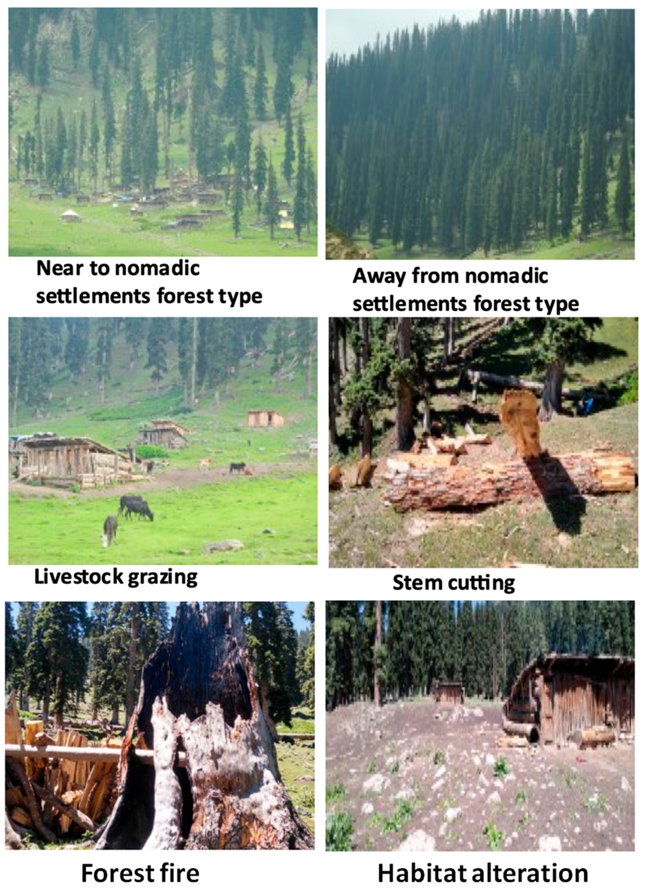
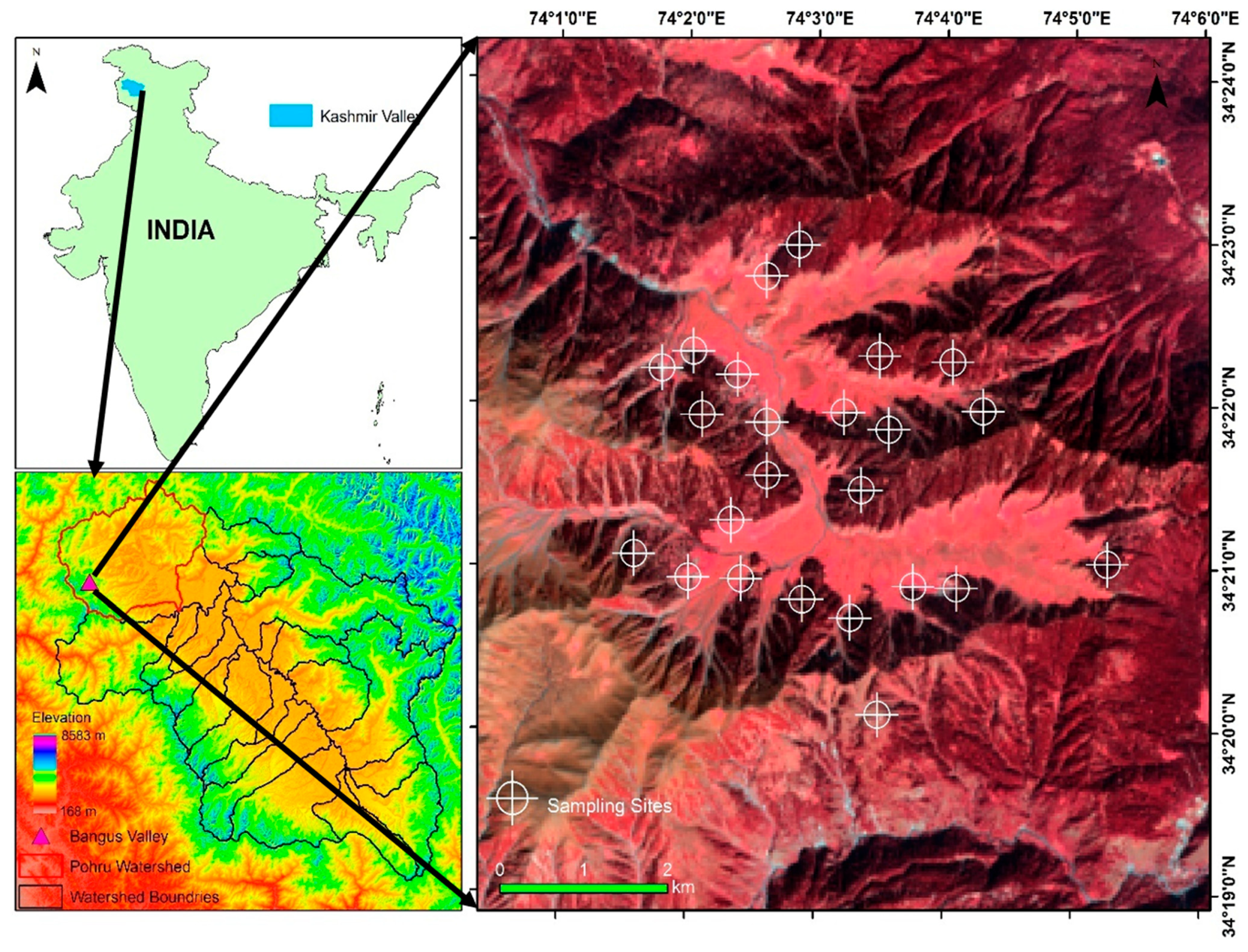
2.1. Study Area
2.2. Sampling Design and Measurements
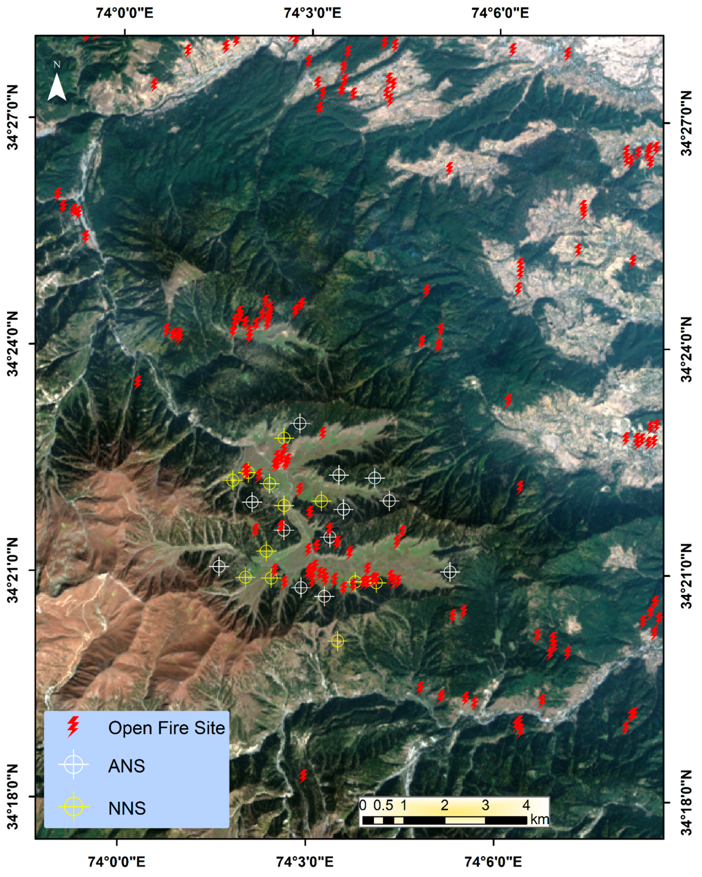
2.3. Remote Sensing for Identifying the Highly Disturbed Hotspots
2.4. Data Analyses
2.4.1. Plant Traits
2.4.2. Diversity Indices, Fire Incidences, NDVI, and EVI between Sites
2.4.3. Plant Species Composition
3. Results
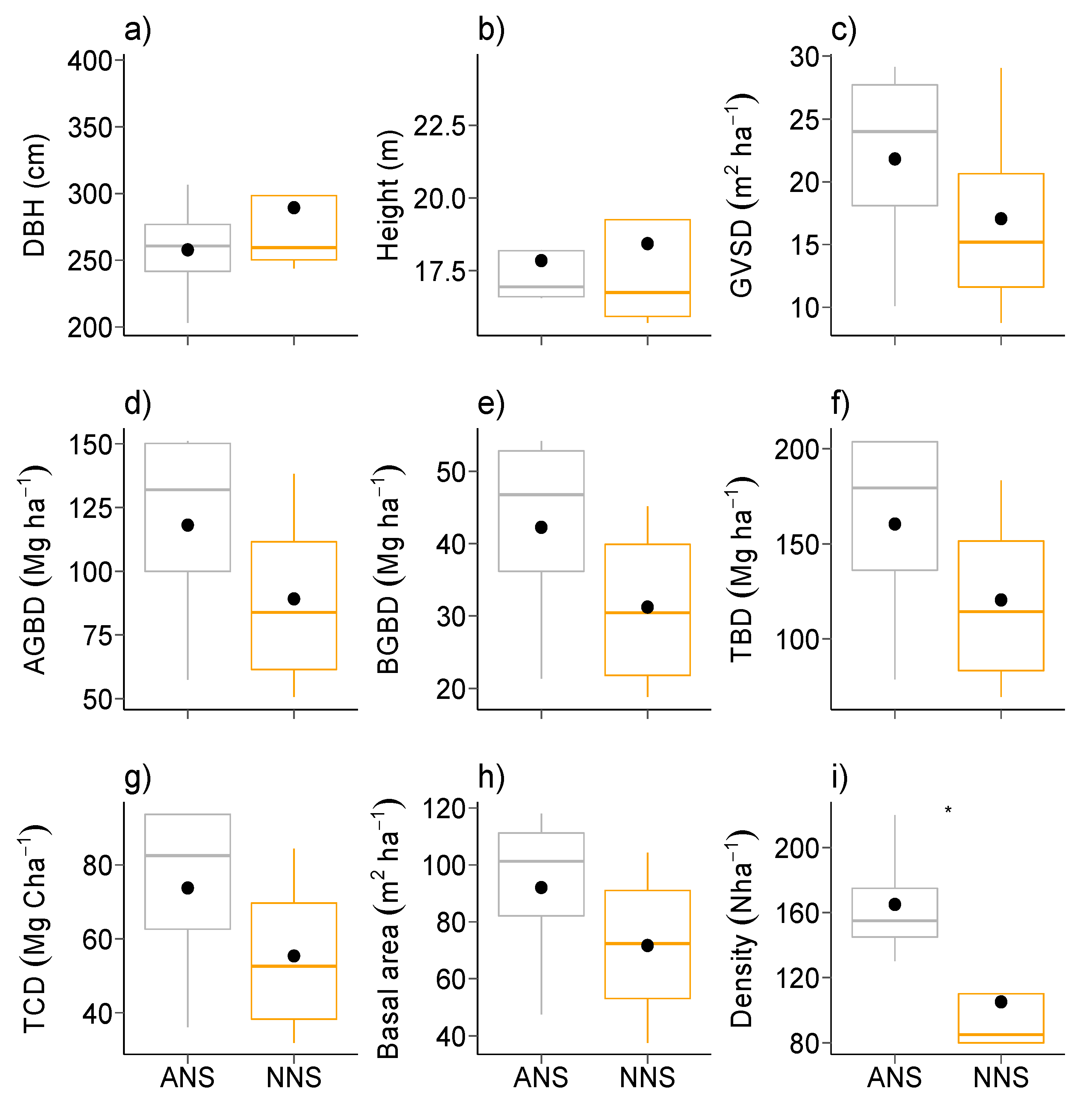
3.1. Plant Traits

| Live Plants | Dead Plants | |||||||
|---|---|---|---|---|---|---|---|---|
| LR Test | p-Value | ANS (Mean ± SD) | NNS (Mean ± SD) | LR Test | p-Value | ANS (Mean ± SD) | NNS (Mean ± SD) | |
| DBH (cm) | 0.583 | 0.4449 | 257.73 ± 42.63 | 289.32 ± 70.88 | 39.807 | 0.0460 | 241.66 ± 37.85 | 280.70 ± 9.91 |
| Height (meter) | 0.063 | 0.8012 | 17.84 ± 2.08 | 18.42 ± 4.12 | 41.574 | 0.0414 | 19.50 ± 1.50 | 17.73 ± 0.86 |
| GSVD (m2ha−1) | 0.596 | 0.4398 | 21.81 ± 8.58 | 17.05 ± 8.82 | 27.205 | 0.0001 | 4.04 ± 1.11 | 8.70 ± 1.40 |
| AGBD (Mgha−1) | 0.963 | 0.3262 | 118.14 ± 43.96 | 89.17 ± 39.37 | 34.28 | 0.0001 | 21.85 ± 5.43 | 47.38 ± 6.82 |
| BGBD (Mgha−1) | 1.266 | 0.2605 | 42.25 ± 15.09 | 31.23 ± 12.47 | 39.685 | 0.0001 | 7.80 ± 1.80 | 7.80 ± 2.27 |
| TBD (Mgha−1) | 1.038 | 0.3083 | 160.39 ± 59.03 | 120.40 ± 51.74 | 35.641 | 0.0001 | 29.66 ± 7.23 | 64.33 ± 9.08 |
| TCD (Mg C ha−1) | 1.038 | 0.3083 | 73.78 ± 27.15 | 55.38 ± 23.80 | 35.641 | 0.0001 | 13.64 ± 3.32 | 29.59 ± 4.18 |
| Basal area (m2ha−1) | 0.892 | 0.3449 | 92.02 ± 31.36 | 71.63 ± 29.64 | 42.599 | 0.0001 | 15.24 ± 4.44 | 36.54 ± 4.77 |
| Density (Nha−1) | 4.235 | 0.0395 | 165.00 ± 38.72 | 105.0 ± 43.58 | 50 | 0.0001 | 32.5 ± 5.0 | 57.5 ± 5.0 |
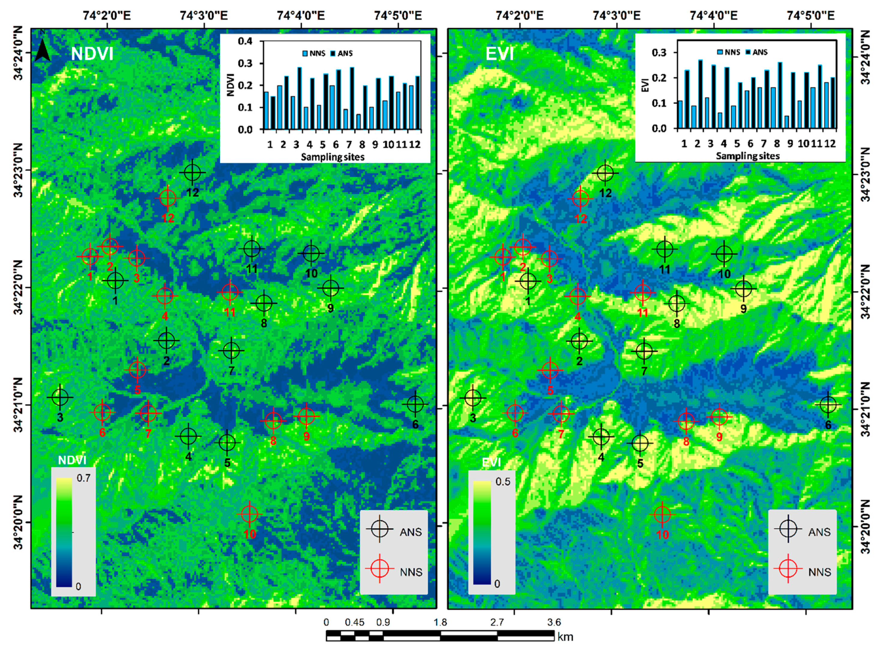
3.2. Diversity Indices, fiRe Incidence, NDVI, and EVI

| Indices | LR Test | p-Value | ANS (Mean ± SD) | NNS (Mean ± SD) |
|---|---|---|---|---|
| Species richness | 2.697 | 0.1005 | 29.75 ± 3.59 | 23.75 ± 2.36 |
| Dominance | 0.280 | 0.5966 | 0.09 ± 0.02 | 0.09 ± 0.01 |
| Shannon | 1.310 | 0.2524 | 2.81 ± 2.70 | 0.16 ± 0.09 |
| Simpson | 0.281 | 0.5957 | 0.90 ± 0.02 | 0.90 ± 0.14 |
| Evenness | 4.746 | 0.0293 | 0.56 ± 0.02 | 0.63 ± 0.05 |
| Margalef | 10.933 | 0.0001 | 6.68 ± 0.66 | 5.37 ± 0.42 |
| Equitability | 2.088 | 0.1485 | 0.83 ± 0.01 | 0.85 ± 0.02 |
| Fisher | 12.582 | 0.0001 | 18.62 ± 2.65 | 12.97 ± 1.75 |
| Fire incidences | 10.818 | 0.0010 | 0.75 ± 0.95 | 4.25 ± 1.89 |
| NDVI | 20.857 | 0.0001 | 0.23 ± 0.01 | 0.13 ± 0.04 |
| EVI | 60.956 | 0.0001 | 0.22 ± 0.01 | 0.12 ± 0.02 |

3.3. Variation of Plant Species Composition between Plant Communities
| Df | Sums Of Sqs | Mean Sqs | F | R2 | Pr (>F) | |
|---|---|---|---|---|---|---|
| Site | 1 | 370.44 | 370.44 | 3.350 | 0.3583 | 0.024 |
| Residuals | 6 | 663.44 | 110.57 | 0.6417 | ||
| Total | 7 | 1033.89 | 1 |
3.4. Satellite-Based Vegetation Indices and Small-Scale Forest Fires
4. Discussion
5. Conclusions
Supplementary Materials
Author Contributions
Funding
Institutional Review Board Statement
Informed Consent Statement
Data Availability Statement
Acknowledgments
Conflicts of Interest
References
- Foster, D.; Swanson, F.; Aber, J.; Burke, I.; Brokaw, N.; Tilman, D.; Knapp, A. The importance of land-use legacies to ecology and conservation. Bioscience 2003, 53, 77–88. [Google Scholar] [CrossRef] [Green Version]
- Elmore, A.J.; Kaushal, S.S. Disappearing headwaters: Patterns of stream burial due to urbanization. Front. Ecol. Environ. 2008, 6, 308–312. [Google Scholar] [CrossRef]
- Willis, K.J.; Birks, H.J.B. What is natural? The need for a long-term perspective in biodiversity conservation. Science 2006, 314, 1261–1265. [Google Scholar] [CrossRef] [Green Version]
- Mladenoff, D.J.; White, M.A.; Crow, T.R.; Pastor, J. Applying Principles of Landscape Design and Management to Integrate Old-Growth Forest Enhancement and Commodity Use. Conserv. Biol. 1994, 8, 752–762. [Google Scholar] [CrossRef]
- Motzkin, G.; Wilson, P.; Foster, D.R.; Allen, A. Vegetation patterns in heterogeneous landscapes: The importance of history and environment. J. Veg. Sci. 1999, 10, 903–920. [Google Scholar] [CrossRef]
- Bradshaw, R.; Hannon, G. Climatic change, human influence and disturbance regime in the control of vegetation dynamics within Fiby Forest, Sweden. J. Ecol. 1992, 80, 625–632. [Google Scholar] [CrossRef]
- Carpelan, C.; Hicks, S. Ancient Saami in Finnish Lapland and their impact on the forest vegetation. In Ecological Relations in Historical Times; Blackwell: Oxford, UK, 1995; pp. 195–205. [Google Scholar]
- Mitchell, C.E.; Tilman, D.; Groth, J.V. Effects of grassland plant species diversity, abundance, and composition on foliar fungal disease. Ecology 2002, 83, 1713–1726. [Google Scholar] [CrossRef]
- Fraterrigo, J.M.; Turner, M.G.; Pearson, S.M. Previous land use alters plant allocation and growth in forest herbs. J. Ecol. 2006, 94, 548–557. [Google Scholar] [CrossRef]
- Brown, S.; Sathaye, J.; Cannell, M.; Kauppi, P.E. Mitigation of carbon emissions to the atmosphere by forest management. Commonw. For. Rev. 1996, 75, 80–91. [Google Scholar]
- Thomson, K. World agriculture: Towards 2015/2030: An FAO perspective. Land Use Policy 2003, 20, 375. [Google Scholar] [CrossRef]
- Kumar, M.; Kalra, N.; Singh, H.; Sharma, S.; Rawat, P.S.; Singh, R.K.; Gupta, A.K.; Kumar, P.; Ravindranath, N.H. Indicator-based vulnerability assessment of forest ecosystem in the Indian Western Himalayas: An analytical hierarchy process integrated approach. Ecol. Indic. 2021, 125, 107568. [Google Scholar] [CrossRef]
- Kumar, M.; Kalra, N.; Ravindranath, N.H. Assessing the response of forests to environmental variables using a dynamic global vegetation model: An Indian perspective. Curr. Sci. 2020, 118, 700–701. [Google Scholar]
- Singh, R.K.; Sinha, V.S.P.; Joshi, P.K.; Kumar, M. Modelling Agriculture, Forestry and Other Land Use (AFOLU) in response to climate change scenarios for the SAARC nations. Environ. Monit. Assess. 2020, 192, 1–18. [Google Scholar] [CrossRef]
- Gupta, A.K.; Negi, M.; Nandy, S.; Kumar, M.; Singh, V.; Valente, D.; Petrosillo, I.; Pandey, R. Mapping socio-environmental vulnerability to climate change in different altitude zones in the Indian Himalayas. Ecol. Indic. 2020, 109, 105787. [Google Scholar] [CrossRef]
- Rawat, A.S.; Kalra, N.; Singh, H.; Kumar, M. Application of Vegetation Models in India for Understanding the Forest Ecosystem Processes. Indian For. 2020, 146, 99–100. [Google Scholar]
- Kumar, M.; Kalra, N.; Khaiter, P.; Ravindranath, N.H.; Singh, V.; Singh, H.; Sharma, S.; Rahnamayan, S. PhenoPine: A simulation model to trace the phenological changes in Pinus roxhburghii in response to ambient temperature rise. Ecol. Modell. 2019, 404, 12–20. [Google Scholar] [CrossRef]
- Kumar, M.; Singh, H.; Pandey, R.; Singh, M.P.; Ravindranath, N.H.; Kalra, N. Assessing vulnerability of forest ecosystem in the Indian Western Himalayan region using trends of net primary productivity. Biodivers. Conserv. 2019, 28, 2163–2182. [Google Scholar] [CrossRef] [Green Version]
- Pandey, R.; Alatalo, J.; Thapliyal, K.; Chauhan, S.; Kelli, M.A.; Gupta, A.K.; Jha, S.K.; Kumar, M. Climate change vulnerability in urban slum communities: Investigating household adaptation and decision-making capacity in the Indian Himalaya. Ecol. Indic. 2018, 90, 379–391. [Google Scholar] [CrossRef]
- Kumar, M.; Rawat, S.P.S.; Singh, H.; Ravindranath, N.H.; Kalra, N. Dynamic forest vegetation models for predicting impacts of climate change on forests: An Indian perspective. Indian J. For. 2018, 41, 1–12. [Google Scholar] [CrossRef]
- Lone, H.A.; Pandit, A.K. Impact of deforestation on some economical important tree species of Langate forest division in Kashmir Himalaya. J. Res. Dev. 2005, 5, 39–44. [Google Scholar]
- Savita; Kumar, M.; Kushwaha, S. Forest resource dependence and ecological assessment of forest fringes in rainfed districts of India. Indian For. 2018, 144, 211–220. [Google Scholar]
- Kumar, M.; Savita; Kushwaha, S.P.S. Managing the Forest Fringes of India: A National Perspective for Meeting the Sustainable Development Goals. In Sustainability Perspectives: Science, Policy and Practice, Strategies for Sustainability; Springer Nature: Cham, Switzerland, 2019; p. 331. [Google Scholar]
- Kumar, M.; Singh, H. Agroforestry as a Nature-Based Solution for Reducing Community Dependence on Forests to Safeguard Forests in Rainfed Areas of India. In Nature-Based Solutions for Resilient Ecosystems and Societies; Springer: Berlin/Heidelberg, Germany, 2020; pp. 289–306. [Google Scholar]
- Terrail, R.; Morin-Rivat, J.; de Lafontaine, G.; Fortin, M.; Arseneault, D. Effects of 20th-century settlement fires on landscape structure and forest composition in eastern Quebec, Canada. J. Veg. Sci. 2020, 31, 40–52. [Google Scholar] [CrossRef]
- Schickhoff, U. Himalayan forest-cover changes in historical perspective: A case study in the Kaghan valley, northern Pakistan. Mt. Res. Dev. 1995, 15, 3–18. [Google Scholar] [CrossRef]
- Josefsson, T. Pristine Forest Landscapes as Ecological References. Ph.D. Thesis, Swedish University of Agricultural Science, Umeå, Sweden, October 2009. [Google Scholar]
- Goldstein, A.; Turner, W.R.; Spawn, S.A.; Anderson-Teixeira, K.J.; Cook-Patton, S.; Fargione, J.; Gibbs, H.K.; Griscom, B.; Hewson, J.H.; Howard, J.F. Protecting irrecoverable carbon in Earth’s ecosystems. Nat. Clim. Chang. 2020, 10, 287–295. [Google Scholar] [CrossRef]
- Kirkham, J.S. Habitat Preference of the Daggerblade Grass Shrimp Palaemonetes pugio and Whether Field Preference is Correlated with the Trematode Parasite Microphallus Turgidus. Master’s Dissertation, Savannah State University, Savannah, GA, USA, May 2018. [Google Scholar]
- Lange, R.T. The piosphere: Sheep track and dung patterns. Rangel. Ecol. Manag. Range Manag. Arch. 1969, 22, 396–400. [Google Scholar] [CrossRef]
- Dormaar, J.F.; Willms, W.D. Effect of forty-four years of grazing on fescue grassland soils. Rangel. Ecol. Manag. Range Manag. Arch. 1998, 51, 122–126. [Google Scholar] [CrossRef] [Green Version]
- Shahriary, E.; Palmer, M.W.; Tongway, D.J.; Azarnivand, H.; Jafari, M.; Saravi, M.M. Plant species composition and soil characteristics around Iranian piospheres. J. Arid Environ. 2012, 82, 106–114. [Google Scholar] [CrossRef]
- Watkinson, A.R.; Ormerod, S.J. Grasslands, grazing and biodiversity: Editors’ introduction. J. Appl. Ecol. 2001, 38, 233–237. [Google Scholar]
- Schäfer, D.; Klaus, V.H.; Kleinebecker, T.; Boeddinghaus, R.S.; Hinderling, J.; Kandeler, E.; Marhan, S.; Nowak, S.; Sonnemann, I.; Wurst, S. Recovery of ecosystem functions after experimental disturbance in 73 grasslands differing in land-use intensity, plant species richness and community composition. J. Ecol. 2019, 107, 2635–2649. [Google Scholar] [CrossRef]
- Romshoo, S.A.; Rashid, I. Assessing the impacts of changing land cover and climate on Hokersar wetland in Indian Himalayas. Arab. J. Geosci. 2014, 7, 143–160. [Google Scholar] [CrossRef]
- Haq, S.M.; Khuroo, A.A.; Malik, A.H.; Rashid, I.; Ahmad, R.; Hamid, M.; Dar, G.H. Forest Ecosystems of Jammu and Kashmir State. In Biodiversity of the Himalaya: Jammu and Kashmir State; Springer: Berlin/Heidelberg, Germany, 2020; pp. 191–208. [Google Scholar]
- Singh, R.K.; Sinha, V.S.P.; Joshi, P.K.; Kumar, M. Use of Savitzky-Golay Filters to Minimize Multi-temporal Data Anomaly in Land use Land cover mapping. Indian J. For. 2019, 42, 362–368. [Google Scholar] [CrossRef]
- Singh, R.K.; Sinha, V.S.P.; Joshi, P.K.; Kumar, M. A multinomial logistic model-based land use and land cover classification for the South Asian Association for Regional Cooperation nations using Moderate Resolution Imaging Spectroradiometer product. Environ. Dev. Sustain. 2020, 23, 6106–6127. [Google Scholar] [CrossRef]
- Kumar, M.; Singh, H.; Padalia, H. Remote sensing for mapping invasive alien plants: Opportunities and Challenges. In Invasive species: A Handbook; Indian Council of Forestry Research and Education: Dehradun, India, 2020; pp. 16–31. [Google Scholar]
- Murillo-Sandoval, P.J.; Hilker, T.; Krawchuk, M.A.; Van Den Hoek, J. Detecting and attributing drivers of forest disturbance in the Colombian andes using landsat time-series. Forests 2018, 9, 269. [Google Scholar] [CrossRef] [Green Version]
- Ishtiyak, P.; Hussain, S.A. Traditional use of medicinal plants among tribal communities of Bangus Valley, Kashmir Himalaya, India. Stud. Ethno Med. 2017, 11, 318–331. [Google Scholar] [CrossRef]
- Haq, S.M.; Calixto, E.S.; Kumar, M. Assessing Biodiversity and Productivity over a Small-scale Gradient in the Protected Forests of Indian Western Himalayas. J. Sustain. For. 2021, 40, 675–694. [Google Scholar] [CrossRef]
- Haq, S.M.; Irfan, R.; Khuroo, A.A.; Lone, J.F.; Gairola, S. Impact of human settlements on the forests of Keran valley Kashmir Himalayas, India. Indian For. 2019, 145, 375–380. [Google Scholar]
- Haq, S.M.; Malik, A.H.; Khuroo, A.A.; Rashid, I. Floristic composition and biological spectrum of Keran-a remote valley of northwestern Himalaya. Acta Ecol. Sin. 2019, 39, 372–379. [Google Scholar] [CrossRef]
- Stewart, R.R.; Ali, S.I.; Nasir, E. An Annotated Catalogue of the Vascular Plants of West Pakistan and Kashmir; Fakhri Printing Press: Sindh, Pakistan, 1972. [Google Scholar]
- Rashid, I.; Bhat, M.A.; Romshoo, S.A. Assessing changes in the above ground biomass and carbon stocks of Lidder valley, Kashmir Himalaya, India. Geocarto Int. 2017, 32, 717–734. [Google Scholar] [CrossRef]
- Mancino, G.; Ferrara, A.; Padula, A.; Nolè, A. Cross-comparison between Landsat 8 (OLI) and Landsat 7 (ETM+) derived vegetation indices in a Mediterranean environment. Remote Sens. 2020, 12, 291. [Google Scholar] [CrossRef] [Green Version]
- Waring, R.H.; Coops, N.C.; Fan, W.; Nightingale, J.M. MODIS enhanced vegetation index predicts tree species richness across forested ecoregions in the contiguous USA. Remote Sens. Environ. 2006, 103, 218–226. [Google Scholar] [CrossRef]
- Fox, J.; Weisberg, S. An R Companion to Applied Regression; Sage Publications: Southend Oaks, CA, USA, 2018; ISBN 1544336489. [Google Scholar]
- R Core Team. R: A Language and Environment for Statistical Computing; R Foundation for Statistical Computing: Vienna, Austria, 2020. [Google Scholar]
- Hervé, M. RVAideMemoire: Testing and Plotting Procedures for Biostatistics. R Package Version 0.9-80. 2020, pp. 9–77. Available online: https://CRAN.R-project.org/package=RVAideMemoire (accessed on 1 August 2021).
- Oksanen, J.; Blanchet, F.; Friendly, M.; Kindt, R.; Legendre, P.; Minchin, D.; Minchin, P.; O’hara, R.; Simpson, G.; Solymos, P.; et al. Vegan: Community Ecology Package (R Package Version 2.5-6); 2019. [Google Scholar]
- Altaf, A.; Haq, S.M.; Shabnum, N.; Jan, H.A. Comparative assessment of Phyto diversity in Tangmarg Forest division in Kashmir Himalaya, India. Acta Ecol. Sin. 2021. [Google Scholar] [CrossRef]
- Chakraborty, A.; Joshi, P.K.; Sachdeva, K. Capturing forest dependency in the central Himalayan region: Variations between Oak (Quercus spp.) and Pine (Pinus spp.) dominated forest landscapes. Ambio 2018, 47, 504–522. [Google Scholar] [CrossRef] [PubMed]
- Bhandari, B.S.; Bijlwan, K. Vulnerability of Forest Vegetation Due to Anthropogenic Disturbances in Western Himalayan Region of India. In Decision Support Methods for Assessing Flood Risk and Vulnerability; IGI Global: Hershey, PA, USA, 2020; pp. 268–289. [Google Scholar] [CrossRef]
- Rawal, R.S.; Gairola, S.; Dhar, U. Effects of disturbance intensities on vegetation patterns in oak forests of Kumaun, west Himalaya. J. Mt. Sci. 2012, 9, 157–165. [Google Scholar] [CrossRef]
- Ramírez-Marcial, N.; González-Espinosa, M.; Williams-Linera, G. Anthropogenic disturbance and tree diversity in montane rain forests in Chiapas, Mexico. For. Ecol. Manag. 2001, 154, 311–326. [Google Scholar] [CrossRef]
- Mligo, C.; Lyaruu, H.V.M.; Ndangalasi, H.J. The effect of anthropogenic disturbances on population structure and regeneration of Scorodophloeus fischeri and Manilkara sulcata in coastal forests of Tanzania. South. For. J. For. Sci. 2011, 73, 33–40. [Google Scholar] [CrossRef]
- Måren, I.E.; Sharma, L.N. Managing biodiversity: Impacts of legal protection in mountain forests of the Himalayas. Forests 2018, 9, 476. [Google Scholar] [CrossRef] [Green Version]
- Mishra, B.P.; Tripathi, O.P.; Tripathi, R.S.; Pandey, H.N. Effects of anthropogenic disturbance on plant diversity and community structure of a sacred grove in Meghalaya, northeast India. Biodivers. Conserv. 2004, 13, 421–436. [Google Scholar] [CrossRef]
- Uniyal, P.; Pokhriyal, P.; Dasgupta, S.; Bhatt, D.; Todaria, N.P. Plant diversity in two forest types along the disturbance gradient in Dewalgarh Watershed, Garhwal Himalaya. Curr. Sci. 2010, 98, 938–943. [Google Scholar]
- Shaheen, H.; Riffat, A.; Salika, M.; Firdous, S.S. Impacts of roads and trails on floral diversity and structure of Ganga-Choti forest in Kashmir Himalayas. Bosque 2018, 39, 71–79. [Google Scholar] [CrossRef] [Green Version]
- Rao, A.N.; Wani, S.P.; Ramesha, M.; Ladha, J.K. Weeds and Weed Management of Rice in Karnataka State, India. Weed Technol. 2015, 29, 1–17. [Google Scholar] [CrossRef]
- Shaheen, H.; Khan, R.W.A.; Hussain, K.; Ullah, T.S.; Nasir, M.; Mehmood, A. Carbon stocks assessment in subtropical forest types of Kashmir Himalayas. Pak. J. Bot 2016, 48, 2351–2357. [Google Scholar]
- Pandey, A.; Arunachalam, K.; Thadani, R.; Singh, V. Forest degradation impacts on carbon stocks, tree density and regeneration status in banj oak forests of Central Himalaya. Ecol. Res. 2020, 35, 208–218. [Google Scholar] [CrossRef]
- Haugaasen, T.; Barlow, J.; Peres, C.A. Surface wildfires in central Amazonia: Short-term impact on forest structure and carbon loss. For. Ecol. Manag. 2003, 179, 321–331. [Google Scholar] [CrossRef]
- Yanai, A.M.; Nogueira, E.M.; de Alencastro Graça, P.M.L.; Fearnside, P.M. Deforestation and carbon stock loss in Brazil’s Amazonian settlements. Environ. Manag. 2017, 59, 393–409. [Google Scholar] [CrossRef] [PubMed] [Green Version]
- Alencar, M.A.; Dias, J.M.D.; Figueiredo, L.C.; Dias, R.C. Frailty and cognitive impairment among community-dwelling elderly. Arq. Neuropsiquiatr. 2013, 71, 362–367. [Google Scholar] [CrossRef] [Green Version]
- Mannan, A.; Liu, J.; Zhongke, F.; Khan, T.U.; Saeed, S.; Mukete, B.; ChaoYong, S.; Yongxiang, F.; Ahmad, A.; Amir, M. Application of land-use/land cover changes in monitoring and projecting forest biomass carbon loss in Pakistan. Glob. Ecol. Conserv. 2019, 17, e00535. [Google Scholar] [CrossRef]
- Sahoo, T.; Acharya, L.; Panda, P.C. Structure and composition of tree species in tropical moist deciduous forests of Eastern Ghats of Odisha, India, in response to human-induced disturbances. Environ. Sustain. 2020, 3, 69–82. [Google Scholar] [CrossRef]
- Pant, H.; Tewari, A. Green Sequestration Potential of Chir Pine Forests Located in Kumaun Himalaya. For. Prod. J. 2020, 70, 64–71. [Google Scholar] [CrossRef]
- Pacheco, P. Smallholder livelihoods, wealth and deforestation in the Eastern Amazon. Hum. Ecol. 2009, 37, 27–41. [Google Scholar] [CrossRef]
- Fearnside, P.M. Deforestation in Brazilian Amazonia: The effect of population and land tenure. Ambio J. Hum. Environ. Res. Manag. 1993, 22, 537–545. [Google Scholar]
- Bhatti, J.S.; Fleming, R.L.; Foster, N.W.; Meng, F.-R.; Bourque, C.P.A.; Arp, P.A. Simulations of pre-and post-harvest soil temperature, soil moisture, and snowpack for jack pine: Comparison with field observations. For. Ecol. Manag. 2000, 138, 413–426. [Google Scholar] [CrossRef]
- Zenner, E.K.; Kabrick, J.M.; Jensen, R.G.; Peck, J.E.; Grabner, J.K. Responses of ground flora to a gradient of harvest intensity in the Missouri Ozarks. For. Ecol. Manag. 2006, 222, 326–334. [Google Scholar] [CrossRef]
- Jaweed, T.H.; Hussain, K.; Kadam, A.K.; Saptarshi, P.G.; Gaikwad, S.W. Characterization of piospheres in northern Liddar valley of Kashmir Himalaya. Earth Syst. Environ. 2018, 2, 387–400. [Google Scholar] [CrossRef]
- Wassen, M.J.; Venterink, H.O.; Lapshina, E.D.; Tanneberger, F. Endangered plants persist under phosphorus limitation. Nature 2005, 437, 547–550. [Google Scholar] [CrossRef]
- Jawuoro, S.O.; Koech, O.K.; Karuku, G.N.; Mbau, J.S. Effect of piospheres on physio-chemical soil properties in the Southern Rangelands of Kenya. Ecol. Process. 2017, 6, 1–7. [Google Scholar] [CrossRef] [Green Version]
- Rejmánek, M.; Richardson, D.M. What attributes make some plant species more invasive? Ecology 1996, 77, 1655–1661. [Google Scholar] [CrossRef]
- Haq, S.M.; Malik, Z.A.; Rahman, I.U. Quantification and characterization of vegetation and functional trait diversity of the riparian zones in protected forest of Kashmir Himalaya, India. Nord. J. Bot. 2019, 37. [Google Scholar] [CrossRef]
- Farooquee, N.A.; Saxena, K.G. Conservation and utilization of medicinal plants in high hills of the central Himalayas. Environ. Conserv. 1996, 23, 75–80. [Google Scholar] [CrossRef]
- Tangki, H.; Chappell, N.A. Biomass variation across selectively logged forest within a 225-km2 region of Borneo and its prediction by Landsat TM. For. Ecol. Manag. 2008, 256, 1960–1970. [Google Scholar] [CrossRef]
- Wani, A.A.; Joshi, P.K.; Singh, O. Estimating biomass and carbon mitigation of temperate coniferous forests in the Western Himalayan region using spectral modeling and field inventory data. Ecol. Inform. 2014, 25, 63–70. [Google Scholar] [CrossRef]

Publisher’s Note: MDPI stays neutral with regard to jurisdictional claims in published maps and institutional affiliations. |
© 2021 by the authors. Licensee MDPI, Basel, Switzerland. This article is an open access article distributed under the terms and conditions of the Creative Commons Attribution (CC BY) license (https://creativecommons.org/licenses/by/4.0/).
Share and Cite
Haq, S.M.; Yaqoob, U.; Calixto, E.S.; Kumar, M.; Rahman, I.U.; Hashem, A.; Abd_Allah, E.F.; Alakeel, M.A.; Alqarawi, A.A.; Abdalla, M.; et al. Long-Term Impact of Transhumance Pastoralism and Associated Disturbances in High-Altitude Forests of Indian Western Himalaya. Sustainability 2021, 13, 12497. https://doi.org/10.3390/su132212497
Haq SM, Yaqoob U, Calixto ES, Kumar M, Rahman IU, Hashem A, Abd_Allah EF, Alakeel MA, Alqarawi AA, Abdalla M, et al. Long-Term Impact of Transhumance Pastoralism and Associated Disturbances in High-Altitude Forests of Indian Western Himalaya. Sustainability. 2021; 13(22):12497. https://doi.org/10.3390/su132212497
Chicago/Turabian StyleHaq, Shiekh Marifatul, Umer Yaqoob, Eduardo Soares Calixto, Manoj Kumar, Inayat Ur Rahman, Abeer Hashem, Elsayed Fathi Abd_Allah, Maha Abdullah Alakeel, Abdulaziz A. Alqarawi, Mohnad Abdalla, and et al. 2021. "Long-Term Impact of Transhumance Pastoralism and Associated Disturbances in High-Altitude Forests of Indian Western Himalaya" Sustainability 13, no. 22: 12497. https://doi.org/10.3390/su132212497
APA StyleHaq, S. M., Yaqoob, U., Calixto, E. S., Kumar, M., Rahman, I. U., Hashem, A., Abd_Allah, E. F., Alakeel, M. A., Alqarawi, A. A., Abdalla, M., Lone, F. A., Khan, M. A., Khan, U., & Ijaz, F. (2021). Long-Term Impact of Transhumance Pastoralism and Associated Disturbances in High-Altitude Forests of Indian Western Himalaya. Sustainability, 13(22), 12497. https://doi.org/10.3390/su132212497