Abstract
In response to the digital revolution, nowadays, many companies operate online and offline businesses in parallel to ensure their future competitiveness. This research examines the inventory strategy for multi-product vendor-buyer supply chain systems, considering space constraints and carbon emissions, in order to improve competence in managing online and offline integrated orders. We amalgamate costs and emissions in transport and storage. Here, we divide the warehouse of the buyer into two stages: one for satisfying online orders and the other for satisfying offline orders. We also assume that additional crashing costs reduce the lead times for receiving products in the buyer’s warehouse. This study demonstrates a mathematical model in the form of a constrained non-linear programme (NLP) and derives a Lagrangian multiplier method to solve it. An iterative solution procedure is designed in order to attain sustainable manufacturing decisions, which are illustrated numerically.
1. Introduction
The modest business environment may amplify the need for industrial storage in order to grasp a higher assortment of products and serve a broader topographical zone of consumers. We should think about stretching out our warehousing abilities to satisfy our commerce and clientele needs more readily throughout this development and extension. The frequent warehouse configurations are either centralized or decentralized. Centralization involves a primary site that supplies all the ordered products to the various sites, such as suppliers, buyers, etc. Decentralization is a method of controlling the batches of various warehouses that send out the products to multiple locations to better aid different markets or store various products. The well-known merit of centralized warehousing is the reduction in operating costs. A significant drawback to centralization is the increased shipping costs. The merits of decentralizing are the reduction in the delay of material handling and an increased ability to store products. The biggest problem with decentralization is the increased operating costs.
Strack & Pochet [1] studied a coordinated supply chain (SC) model for warehouse and inventory planning. Their research goal was to appraise the value of integrating tactical warehouse and inventory decisions. Sainathuni et al. [2] designed an NLP model for the warehouse transportation problem involving multiple vendors, stores, and periods in an SC system. Yanlai & Fangming [3] considered the trade credit period in a two-warehouse SC model for deteriorating items. Payel & Bibhas [4] derived a two-warehouse integrated SC model considering quantity discount and demand depending on the stock in an imperfect manufacturing process. Chakraborty et al. [5] studied a two-warehouse trade-credit model with Weibull distribution deterioration and inflation. Alawneh & Zhang [6] derived a dual-channel SC model for fulfilling online and offline orders. Peng et al. [7] designed a buy-online-and-deliver-from-store strategy for a dual-channel SC considering the retailer’s location advantage.
Communication technology is the transfer of messages (information) among people and/or machines through the use of technology. This processing of information can help people make decisions, solve problems, and control machines. Sandeep et al. [8] discuss the vital technologies and opportunities within Food Logistics 4.0. In this connection, an SC can be defined as the integration of all activities associated with the flow and transformation of finished products, from the raw materials through to the end-user, as well as the associated information flows, through improved supply chain relationships in order to achieve a sustainable competitive advantage. This study will investigate the impact and role of information technology on inventory management. Supply chain management (SCM) addresses the handling of information and material across the entire chain, including producers, suppliers, retailers, distributors, and customers. This study aims to examine the effectiveness and role of the developed technology in the handling of material.
The multi-echelon SC is a familiar network structure for large-scale companies. Chen et al. [9] addressed a coordination inventory problem for online sales in a drop-shipping environment. Fichtinger et al. [10] identified the environmental impact of warehouse inventory management. Ouyang et al. [11] designed an integrated SC model under capacity constraints with a trade credit period. Priyan & Uthayakumar [12] presented a two-echelon SC model for multi-items, including recovery options with trade credit and variable lead times considering multi-constraints. Xu et al. [13] provided the optimal inventory strategies under a centralized and decentralized SC system. Aslani & Heydari [14] addressed collaborated dual-channel SCs with regard to the issues of pricing and product greenness under channel disruption. He et al. [15] designed a structure for a dual-channel closed-loop SC under a government subsidy. Mojtaba & Mehdi [16] investigated an inter-SC cooperation strategy to reduce the time-dependent deterioration costs by considering sharing warehouses. Javad et al. [17] derived dual-channel SC coordination considering targeted capacity allocation under uncertainty. Taleizadeh et al. [18] addressed a multi-buyer multi-vendor SC problem with limited capacity. Kurt et al. [19] present a model and solution methodology for production and inventory management problems that involve multiple resource constraints. Müge & Onur [20] built a two-stage stochastic model with budget constraints for the two-product case and determined its optimal solution using Lagrangian multiplier conditions. Priyan & Uthayakumar [12,21] solved SC problems using the Lagrangian multipliers method under various environments.
Another problem with inventory communication between the buyer and the seller is the lead time. The decline in the lead time and backorder price discounts becomes significant when the SC results from an uncertain demand. Hoque & Goyal [22], and Hoque [23], examined the batch-size effect and shortened lead times on renewing the stock strategies of the relationship between the supplier and the purchaser. Modak & Kelle [24] have indicated a double-channel SC where the client can buy online or from the stores derived via DFA. Priyan & Mala [25] suggest a healthcare SC model considering the varying quality characteristics for the raw materials and finished products, varying lead times, and service level constraints. Myron et al. [26] developed a model for pricing, lead-time quotations and delay compensation in a Markovian make-to-order production or service system with strategic customers who exhibit risk aversion. Bikash et al. [27] propose a smart SC model with variable lead times and variance.
Emissions from carbon trap heat in the atmosphere, making the planet warmer. The increase in greenhouse gases within the atmosphere in the last 150 years has resulted from increased human practices [28], as shown in Figure 1. Fossil fuel combustion from generating electricity, heat, and transport is the main source of carbon released into the atmosphere. The primary sources of carbon pollution from industries are the burning of fossil fuels to generate energy, and the greenhouse gases emitted from the chemical reactions that produce goods from raw materials. The emissions rise and fall from year to year depending on fuel prices, changes in the economy, and other factors. Climate change resulting from carbon pollution has led to high costs that are already being felt globally. There is a need for developing policies that will shift the carbon pollution costs facing the polluters. This will reduce carbon emissions across all sectors, such as industry, energy, and transportation. The best option would be setting a price for carbon that shifts the cost to the polluters, which will reduce greenhouse gas emissions.
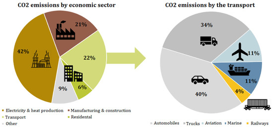
Figure 1.
Global greenhouse gas emissions by the transportation sector.
The literature on the emissions of carbon in the inventory system has risen significantly over the past few years. Hammami et al. [29] designed two multi-stage SC models with lead-time limitations in carbon emission tax and cap regulation. Li et al. [30] report the development of two models for the SC system, and the incorporation of carbon emissions where there are operation problems with production and transport operations found in the cap-and-trade rules and the regulation for combined carbon cap-and-trade and tax. Tang et al. [31] developed the reduction of emissions in the transport industry and inventory management found in the (R, Q) inventory policy. Halat & Hafezalkotob [32] studied the effect of synchronization and the regulation of carbon-on-carbon emissions, inventory costs, and the objective role of the government by the game theory approach. A few more papers have also been published in the field of carbon emissions [33,34,35,36]. Table 1 summarizes an overview of the reviewed literature.

Table 1.
Literature review overview.
Firms introducing online sales are facing many challenges in terms of logistics and delivery processes, such as large volumes of very small orders, short delivery lead times, flexible delivery, the capacity of the warehouse, and the picking and packing process for single unit orders, in addition to the usual challenges of the conventional business. Warehouses or distribution centers must be ready to prepare orders coming from both offline stores and online shoppers. The conventional warehouse was designed for physical stores and delivery does not work under a dual-channel business environment. For example, warehouse workers cannot use the same picking patterns for online orders as for physical shoppers. Warehouses operating in the current digital era of e-commerce must have the all-purpose infrastructure, which is capable of sharing information, interconnectedness, and handling different orders from different customer segments with various features, such as diverse order sizes and delivery lead times (McCrea [37]).
The emergence of COVID-19 in 2020 prompted a global economic collapse, with the economic effect exceeding that of the 2008 financial crisis [38]. COVID-19 clearly had a detrimental impact on international commerce, the service sectors, manufacturing, and supply chains, and many firms have suffered from insolvency or a lack of money (Zhang et al. [39]). In the economic recovery and transformation of enterprises, green finance can promote the green capital market to actively fight the epidemic and serve and support the real economy with a shortage of funds [38,40]. Among the challenges in running the dual-channel warehouse are how to organize the warehouse to control carbon emissions, and how to manage inventory to fulfill both online and offline (retailer) orders, where the orders from different channels have different features.
Although numerous studies address the multi-echelon SC, only a few have applied an inventory model in a multi-channel multi-echelon SC considering multiple products. To the best of our knowledge, no research has considered carbon emissions and controllable lead times aiming to optimize carbon emission policies with minimum system costs. The key contribution of this research is to fill this research gap. We attempt to respond to the following questions from the assumption and the model set:
- If the lead-time demand is uncertain, what would be the economic inventory approach for the industry?
- How can we adjust the operations to reduce carbon emissions?
- What impacts do space constraints have during decision-making?
- How can we improve efficiency in handling online and offline integrated orders?
The rest of the paper follows the consequent design: Section 2 shows the required notations and assumptions of the research. The mathematical model is constructed in Section 3, and Section 4 studies the solution procedure of the problem. Section 5 discusses the sensitivity and numerical analyses. Section 6 concludes the paper.
2. Notations and Assumptions
2.1. Notations
| M | Number of finished products (or products) and raw material families controlled in the system |
| i | Index for item |
| j | Index for stage, where j = 1 for warehouse area to satisfy online demand, and j = 2 for warehouse area to satisfy both retail and online demands |
| Pi | Production rate for the ith item |
| Si | Setup cost for the ith item |
| hi | Holding cost for the ith item |
| c | Price of the fuel |
| c0 | Cost of carbon emissions per unit released |
| g0 | Unit fuel consumption for the unloaded vehicle |
| g1 | Unit fuel consumption for the loaded vehicle |
| α | Minimum required space probability |
| W | Floor space of the entire warehouse |
| R(L) | Crashing cost |
| T1i | Production time For ith raw material family |
| Ordering cost | |
| Holding cost per unit time | |
| ϑi | Defect rate in a lot |
| Replenished quantity for production | |
| Screening rate | |
| Screening cost | |
| Disposal cost | |
| Labor cost For item i in stage j | |
| xij | Demand during lead time |
| Dij | Rate of demand |
| σij | Standard deviation of demand during lead time |
| Aij | Order cost per order |
| hij | Holding cost per unit time |
| γij | Storage space |
| rij | Reorder point |
| βij | The fraction of shortage backordered (0 ≤ βij ≤ 1) |
| Penalty cost for a loss of sale including lost profit | |
| Shortage cost per unit backordered | |
| f(xij) | Probability density function (p. d. f) of lead-time demand Decision variables |
| Qij | Ordered quantity for item i in Stage j |
| n | Total number of shipments |
| L | Lead time |
| θ | Lagrangian multiplier |
2.2. Assumptions
- This single vendor-buyer system is dealing with M finished products and raw material families. A raw material family is a group of raw materials that are converted to a single finished product.
- The buyer’s warehouse is divided into two stages. Stage 1 is for sending small-size online customer orders, while Stage 2 is for fulfilling offline large-size orders. Both Stages 1 and 2 obtain internal shipments from Stage 2 and the supplier, respectively. In addition, the reorder point of each stage parallels an installation inventory for that stage (see Alawneh & Zhang [6,42,43]).
- An external supplier delivers all ordered quantities in a single delivery for raw material family .
- For the ith product at stage j, the reorder point is = expected demand during L, and , i.e., , where is the safety factor and satisfies , and signifies the acceptable stock-out chance for item during L at stage .
- The lot-size, , is placed when its inventory level falls to because the buyer follows a continuous review strategy.
- For M products, the lead time, , is comprised of jointly sovereign modules. The Jth module has a normal period , a minimum period , and a crashing cost per unit time . It rearranges such that . The modules of L are crashed one at a time, starting from the 1st module, because it has the minimum unit crashing cost, and then the 2nd module, and so on.
- Let , and be the length of L with modules crashed to their minimum period, then can be derived as ; and for M products, the crashing cost per cycle is derived by , as given in [26].
3. Model Development
The geometrical picture of the proposed dual-channel two-echelon SC system is expressed in Figure 2.
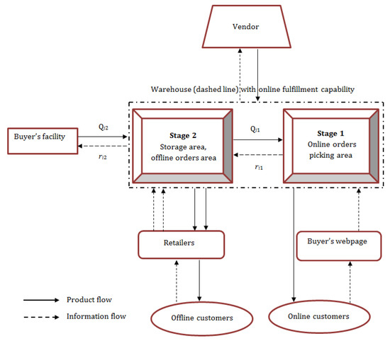
Figure 2.
Geometrical picture of the dual-channel system.
3.1. Model Formulation for the Vendor
3.1.1. Cost of Raw Material Family
For raw material family i, the replenishment quantity is received at the beginning of each cycle time instantaneously. The expected order cost per unit time .
Raw material families are screened at a rate of to the distinct perfect and imperfect raw material family because of the imperfect quality in each ordered quantity, . At the end of the screening process, imperfect raw material families are disposed of as a single lot at the lowest disposal price per unit item. Screening cost . The disposal cost for imperfect raw material families per unit time .
Let where . That is,
Holding costs for a perfect and imperfect raw material family per unit time are and , respectively. Then the labor cost for all raw material families is .
Let be the vendor’s expected total cost for the ith raw material family, which is the accumulation of the expected order, holding, screening, labor, and disposal costs.
That is,
Using Equations (1) and (2), we have
Now, the expected total cost for M raw material families per unit time is
3.1.2. Cost of Finished Products
In the proposed scenario, the vendor initiates the production at the rate and obtains the product in n lots, each of size . The initial lot is ready for shipment after the period of and the vendor continues to deliver the product on average every unit of time until the inventory level becomes 0.
Hence, the vendor’s expected on-hand inventories for product is the difference of the accumulated inventory of the vendor and the buyer. According to Priyan & Uthayakumar [12], the inventory of product for the vendor is units, as well as the accumulated inventory for the buyer, which is . Henceforth, the vendor’s expected inventory per unit time is
The holding and setup costs for the ith product per unit time are and , respectively.
Let and be the unit fuel consumption for the unloaded (return trip) and loaded vehicle, respectively. In this research, the amount of fuel ingested for the vendor’s transportation vehicle to and from is and , respectively. Thus, the total amount of fuel ingested for replenishment is .
Hence, the transportation cost per unit of time for ith is product .
The vendor’s expected total cost, for the finished product , equals the sum of the setup, holding, and transportation costs. That is,
The expected total cost per unit time for M finished products is
3.1.3. Cost of Carbon Emission
In this model, we consider that transport and storage produce the total quantity of carbon emissions. Thus, on the basis of the features of transport and storage, the quantity of emissions is the sum of emissions from transportation, denoted by and storage denoted by . That is,
Here, and are the carbon emission factors for fuel and energy. In , and are fixed and the unit variable is the energy ingested for storage.
Consequently, the vendor’s overall carbon emissions cost for M products is derived by:
Then the expected total cost for the vendor for M products is
3.2. Inventory Model for the Buyer
The buyer uses a dual-channel warehouse that is divided into two stages. Stage 1 is for sending small-size online customer orders, while Stage 2 is for fulfilling offline large-size orders. The ith product’s ordering cost at jth stage for .
Now the average inventory level for Stage 2 and Stage 1 are the sum of the average cycle inventory and the safety inventory, expressed as , and , respectively. Hence the holding cost for the ith product at Stage 2 is and Stage 1 is . The expected shortage of the ith product at Stage 2 and the expected backorders . The backorder cost for the ith product at Stage 2.
For the ith product at Stage 2, shortages occur when . Therefore, for the ith product at Stage 2, the buyer’s expected shortage at the end of the cycle time is
The backorder cost per unit time .
Similarly, the expected backorder cost per unit time for the ith product at Stage 1 is . Thus, the buyer’s expected total cost is comprised of the ordering, holding, backorder, and crashing costs.
That is,
Now the joint expected total cost, IETC(, , L, n), per unit time for products can be stated as the sum of (given in Equation (3)) and (given by Equation (4)). That is,
Now we include the buyer’s warehouse capacity constraint. Then, similar to Alawneh and Zhang [6], we have the constraint , where , and is the value of the cumulative probability distribution of the demand at point .
Then .
That is, warehouse space constraint is
Now our aim is to obtain the optimal of , , L, and for products that minimize the , as given in Equation (5), and satisfy the storage constraint, as shown in Equation (6). The mathematical model of the problem is
subject to,
4. Solution Technique
The problem, which is expressed in Equation (7), is a constrained NLP. We use the Lagrangian multiplier optimization technique to solve the proposed NLP. That is, we optimize the succeeding function by adding a Lagrange multiplier:
Property 1.
For fixed , , and , is convex in .
Proof.
Take the first- and second-order derivatives of Equation (8) with respect to , and we have,
Therefore, for fixed , , and , is convex in n. □
Property 2.
For fixed , , and , is convex in .
Proof.
Take the first- and second-order derivatives of with respect to , and we have,
and .
Therefore, for fixed , , and , is convex in . □
Result 3.
For the given values of , , and , and , by equating Equation (9) to zero, we attain the subsequent optimal lot size :
Property 4.
For fixed , n, and , is convex in .
Proof.
Take the first- and second-order derivatives of with respect to , and we have,
and
Therefore, for fixed , , and , is convex in . □
Result 5.
For the given values of , , and , , by equating Equation (11) to zero, we attain the subsequent optimal lot size :
Property 6.
For fixed , , and , is concave in .
Proof.
Take the first- and second-order derivatives of with respect to , and we have,
and
Therefore, for fixed , , and n, is concave in . □
Result 7.
Since for fixed , , and , is concave in , the minimum will occur at the endpoints of the interval . Now we take the first derivative of with respect to the Lagrangian multiplier θ,
Algorithm
Step 1. Set .
Step 2. For each execute Steps (2.1) to (2.3).
Step 2.1. Calculate the value by solving Equation (13).
Step 2.2. Using the value of , determine and from Equations (10) and (12), respectively.
Step 2.3. Compute the corresponding using Equation (8).
Step 3. Find .
Step 4. Set . Then the set is the optimal solution for .
Step 5. Set and recap Steps 2–4 to find .
Step 6. If , then jump to Step 5, or else move to Step 7.
Step 7. If , then the set is an optimal solution.
5. Numerical Analysis
We carry out a numerical analysis to validate the applications and performance of the proposed solution technology. The parameters are tabulated in Table 2. In Table 2, we take a few appropriate values from Alawneh & Zhang [6], and carbon emission values from www.eia.gov, accessed on 21 July 2021, which is the website of the U.S. Energy Information Administration, and other values based on the following realistic observations:
Table 2.
Numerical parameters.
- : The Stage 1 purchasing procedure seeks to refill products for Stage 2, but Stage 2 replenishment necessitates ordering items from the provider. As a result, the cost of buying Stage 2 from an external source is greater.
- : Because the necessary space to keep a unit in the online low-density region is larger than that in the offline high-density area, the holding cost for the online channel is higher than that for the offline channel.
- : The online channel’s backorder cost is designed to be lower than the offline channels. Online orders are often smaller than offline orders, and online orders offer greater flexibility in delivery schedules than offline orders. Because a shortage in an offline order usually results in a higher penalty, based on the contract signed between the vendors and the buyers, whereas a shortage in an online order has a smaller economic impact on the vendors, it is reasonable to have a Stage 2 shortage cost that is higher than the Stage 1 shortage cost.
- : Offline demand is often higher than online demand, and offline channel demand has a bigger order size than online demand.
- : The assumption is based on the fact that, in Stage 2, the space required for each unit placed on pallets is smaller than in Stage 1, when the goods are generally stored in low-density storage systems, such as stands or racks, to allow individual item selection.
- In the numerical experiment, we set tonnes/gallons, t/kWh as default values. The values of and are taken from www.eia.gov, accessed on 21 July 2021, which is the website of the U.S. Energy Information Administration. As well, we set , and as the default values, similar to the existing work of Tang et al. [32].
- Moreover, and are the unit fuel consumptions for the unloaded and loaded vehicles, respectively. We set gallons, gallon/unit as the default values. In practice, is usually much greater than 0. The following is an explanation. To fulfill the required emission reduction objective, the reorder point is reduced, lowering the average inventory level and, therefore, reducing the emissions from storage. Simultaneously, the order quantity rises dramatically, resulting in a further reduction in shipment frequency in order to save gasoline.
Furthermore, the lead-time demand has three modules, with the data shown in Table 3, similar to Banerjee [44], and Table 4 provides the data of the lead-time modules [25].
Table 3.
Lead-time components data [44].
Table 4.
Summarized lead-time data [25].
On the basis of the algorithm, we obtain the optimality of , lot-sizes and the corresponding expected total cost = 386,840. The graphical depiction of the expected total cost versus n is expressed in Figure 3.
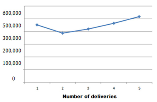
Figure 3.
Graphical representation of LF(.) vs. .
5.1. Sensitivity Analysis
In this section, the sensitivity analysis is performed in order to know the effects of the major parameters. This study is applicable when only one parameter has changed at a time, and other parameters have been kept at their original values. The results are listed in Table 5, Table 6, Table 7, Table 8, Table 9, Table 10 and Table 11, and the plots are shown in Figure 4. The sensitivity analysis will allow for some productive managerial insights.
Table 5.
Sensitivity analysis where production rate Pi is changed.
Table 6.
Sensitivity analysis where Dij is changed.
Table 7.
Sensitivity analysis where ordering cost Aij is changed.
Table 8.
Sensitivity analysis where shortage cost πyij is changed.
Table 9.
Sensitivity analysis where penalty cost π0ij is changed.
Table 10.
Sensitivity analysis where raw material ordering cost Awi is changed.
Table 11.
Sensitivity analysis where setup cost Si is changed.
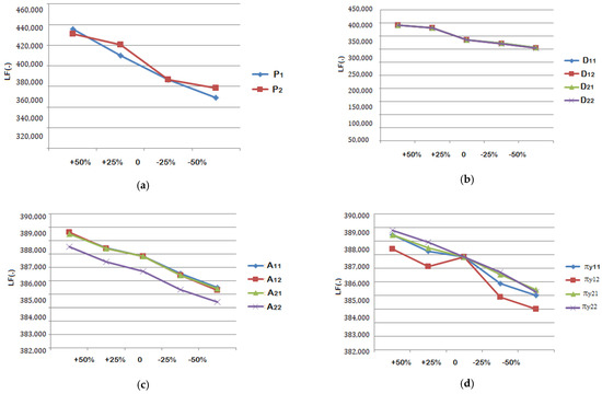
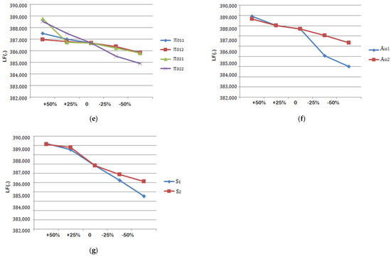
Figure 4.
Plots of the sensitivity analyses for major parameters: (a) Effects of production rate Pij; (b) Effects of production rate ; (c) Effects of ordering cost ; (d) Effects of shortage cost ; (e) Effects of penalty cost ; (f) Effects of raw material ordering cost ; (g) Effects of setup cost .
5.2. Managerial Insights and Discussion
On the basis of the behavioral changes, as reflected in Table 5, Table 6, Table 7, Table 8, Table 9, Table 10 and Table 11 and Figure 4, the resulting managerial insights can be derived:
- (1)
- The members of the SC system can condense their inventory costs, as well as their carbon emissions, by executing a collaboration apparatus for handling product streams. As a result, collaboration assists both the government and the SC system in attaining their goals. Though the collaborative design may be hard to execute in practice, it necessitates a decision-maker with all of the partners’ details.
- (2)
- An increasing value of results (Table 5) in an increase in the number of deliveries, and an increasing value of increases the total costs, which indicates the increasing value of the maximum inventory level. It increases the back-ordered quantity while carbon emission factors are unchanged. Therefore, producers shouldn’t increase the production rates so high that the holding costs increase by a large amount.
- (3)
- The results from Table 5, Table 6, Table 7, Table 8, Table 9, Table 10 and Table 11 demonstrate the impact of inventory decisions on the expected system costs, including the carbon emission costs. Consequently, industries can reduce their emissions through operational alterations as an alternative to other expensive techniques. Benjaafar et al. [41] agree on this viewpoint in their paper.
- (4)
- The effects of the inventory strategies evaluated by this study are based on emissions, the objective functions of the proposed inventory system, and inventory costs. The results indicate that is extremely sensitive to the parameters of , , and , and is less sensitive to other parameters. The value of is extremely sensitive to the parameters , , and , and less sensitive to the other parameters,
- (5)
- A dual-channel company decision-maker must consider whether to sell products offline, online, or through both channels, as well as the impact of online and offline sales on the system costs. In such a situation, the suggested model is a valuable decision support tool for estimating the incurred inventory-related costs. Table 6 and Figure 4b show the outcomes for an item with various offline demand increments for three distinct scenarios of online demand, namely, unchanged, increased, and reduced, as a result of the addition of the offline demand. Decision-makers can choose which channel to sell the products through based on the cost increase. The findings back the notion that low-demand products should be offered online, whereas high-demand items should be sold both online and offline. Xingyue & Haluk [45] examined and compared consumer demand under product substitution when the price changes, or the product stocks out, between online and offline markets, using a large-scale dataset on consumer packaged goods and a random coefficients discrete choice model.
- (6)
- In some situations, according to the nature of the business, we must choose a channel preference in terms of which channel is preferred in order to meet demand. By changing the scarcity and penalty costs, we can simply include channel preference into our model. Table 8 and Table 9 and Figure 4d,e illustrate an example of shortage and penalty costs and their effects on the channel preference. As we can observe in Table 8 and Table 9 and Figure 4d,e, we keep the shortage and penalty costs constant for the offline channel and increase the deficit and penalty costs for the online channel. As the cost of online backorders rises, the offline fill rate falls, and the online fill rate rises. The greater the online service level, the higher the online scarcity and penalty charges will be.
- (7)
- Modifications in batch sizes or order amounts, for example, have been shown to reduce emissions successfully. In the context of a dual-channel two-echelon inventory system, this article presents a new mathematical model that combines costs and emissions in transit and storage to perform optimal operational changes.
- (8)
- When transportation is the primary source of emissions, the overall quantity of emissions falls as rises. When transportation and storage account for the majority of emissions, the total amount of emissions from transportation and storage rises as the reorder point rises, although it may rise or fall with order quantity , depending on the values of the parameters. Transportation-related emissions always decrease as the order quantity increases.
- (9)
- The value of the total system cost, is highly sensitive with respect to the parameters of , and , more sensitive to , and less sensitive to the parameters of , and . Priyan and Uthayakumar [46] address the same phenomena in their paper.
- (10)
- There is a two-way relationship between energy consumption and carbon emissions. The increase in energy consumption will significantly promote the rise of carbon emissions, leading to the continuous deterioration of the environment. Given this fact, we considered in the amounts of emissions where is holding inventory.
- (11)
- The greater the load, the greater the fuel consumption to move that load around, especially in stop-and-go traffic where the load must be frequently accelerated and decelerated. Even on long straight hauls, any increase in the load also increases the vehicle’s rolling resistance at the cost of additional fuel. Because of this indisputable fact, in the amounts of emissions, we considered the factor where is delivery quantity. If the quantity increases then, automatically, the fuel consumption for the loaded vehicle increases.
- (12)
- Many firms would willingly establish a carbon footprint reduction objective as an important component of their social responsibility initiatives once the carbon emission factor is taken into consideration. More significantly, large retailers, such as Walmart, have established an emission reduction target for their suppliers as well as a timeline. By the end of 2021, the firm wants to cut carbon emissions by 40 million metric tons throughout its supply chain.
- (13)
- As we discussed earlier in Section 1, among the challenges of running a dual-channel warehouse are organizing the warehouse in order to help the government limit carbon emissions and managing inventory to fulfill online and offline (retailer) orders with different features. We provide the optimal inventory decisions for the firms facing challenges in a dual-channel system, with the objective of minimizing system costs and controlling carbon emissions. This study contributes to the existing literature on warehouse management in several ways. First, it is the first work to analyze the structure of the emerging dual-channel warehouses and to develop a structure related to the inventory policy for such warehouses. Second, it develops a mathematical model that determines the multi-item product inventory policy for the two areas in integrated dual-channel warehouses, minimizing their total expected costs. The constraint of warehouse space is also considered. Furthermore, the proposed solution can be used to evaluate the performance of two-echelon dual-channel warehouse systems by comparing the total system costs for different warehouse structures and assessing the effects of adding a new sales channel. The solutions demonstrate that the proposed model is appropriate to industries using a dual-channel inventory system.
6. Conclusions
The major goals of buyer’s warehouses are to maximize space utilization, lower operating costs, and fulfill orders swiftly and reliably. These goals are frequently at odds with one another. We need to store goods in high-density storage areas, such as on pallets or in high beam storage systems, to achieve high space utilization. Meanwhile, the effective order selection for online orders, which are often modest in size, needs complete access to the stored products, which necessitates displaying them in low-density storage spaces, such as on racks or stands. At the same time, the warehouse must maintain an ideal inventory level for each item in order to deliver a high level of service. To fulfill both online and offline orders, we evaluate the developing dual-channel warehouse.
For the purpose of determining the ordering quantities for both offline and online channels, we study the two-channel warehouse two-echelon SC system considering carbon emissions. We consider that transportation and storage produce a certain amount of carbon emissions in the system, and that the lead time can be controlled by crashing costs. Moreover, we consider the warehouse capacity for the buyer. This research aims to minimize inventory and carbon emission costs while satisfying warehouse space constraints. We formulate a constrained NLP and design a Lagrangian multiplier technique to find the optimal decision variables. Numerical examples demonstrate the merit of the proposed model for determining the optimal strategies for dual-channel warehouse multi-echelon systems.
In the future, one can extend this study to multi-constraints. Moreover, the setup/ordering cost, which was constant in this study, should be considered a decision variable and used to determine the impacts of decreasing setup costs. This research can be studied by considering that buyers purchase products from multiple vendors. In addition, the present study can be extended through to the service level limit and the trade credit period in the inventory model.
Author Contributions
Conceptualization, P.M. and N.A.; Data Curation, P.M. and M.P.; Formal Analysis, S.P. and G.P.J.; Funding Acquisition, J.R.; Investigation, M.P.; Methodology, M.P., S.P. and S.A.; Project Administration, S.P., N.A. and J.R.; Resources, G.P.J. and J.R.; Supervision, G.P.J.; Validation, S.P., N.A. and S.A.; Visualization, S.P.; Writing—original draft, P.M.; Writing—review & editing, S.A. and G.P.J. All authors have read and agreed to the published version of the manuscript.
Funding
This work was supported by the research fund of Hanyang University (HY-2018).
Institutional Review Board Statement
Not applicable.
Informed Consent Statement
Not applicable.
Data Availability Statement
No data were deposited in an official repository.
Conflicts of Interest
The authors declare no conflict of interest.
References
- Strack, G.; Pochet, Y. An integrated model for warehouse and inventory planning. Eur. J. Oper. Res. 2010, 204, 35–50. [Google Scholar] [CrossRef] [Green Version]
- Sainathuni, B.; Parik, P.J.; Zhang, X.; Kong, N. The warehouse-inventory-transportation problem for supply chains. Eur. J. Oper. Res. 2014, 237, 690–700. [Google Scholar] [CrossRef]
- Liang, Y.; Zhou, F. A two-warehouse inventory model for deteriorating items under conditionally permissible delay in payment. Appl. Math. Model. 2011, 35, 2221–2231. [Google Scholar]
- Mandal, P.; Giri, B.C. A two-warehouse integrated inventory model with imperfect production process under stock-dependent demand and quantity discount offer. Int. J. Syst. Sci. Oper. Logist. 2019, 6, 15–26. [Google Scholar]
- Chakraborty, D.; Jana, D.K.; Roy, T.K. Two-warehouse partial backlogging inventory model with ramp type demand rate, three-parameter Weibull distribution deterioration under inflation and permissible delay in payments. Comput. Ind. Eng. 2018, 123, 157–179. [Google Scholar] [CrossRef]
- Alawneh, F.; Zhang, G. Dual-channel warehouse, and inventory management with stochastic demand. Transp. Res. Part E 2018, 112, 84–106. [Google Scholar] [CrossRef] [Green Version]
- He, P.; He, Y.; Xu, H. Buy-online-and-deliver-from-store strategy for a dual-channel supply chain considering retailer’s location advantage. Transp. Res. Part E: Logist. Transp. Rev. 2020, 144, 102127. [Google Scholar]
- Jagtap, S.; Bader, F.; Garcia-Garcia, G.; Trollman, H.; Fadiji, T.; Salonitis, K. Food Logistics 4.0: Opportunities and Challenges. Logistics 2021, 5, 2. [Google Scholar] [CrossRef]
- Chen, Y.K.; Chiu, F.R.; Lin, W.H.; Huang, Y.C. An integrated model for online product placement and inventory control problem in a drop-shipping optional environment. Comput. Ind. Eng. 2018, 117, 71–80. [Google Scholar] [CrossRef]
- Fichtinger, J.; Ries, J.M.; Grosse, E.H.; Baker, P. Assessing the environmental impact of integrated inventory and warehouse management. Int. J. Prod. Econ. 2015, 170, 717–729. [Google Scholar] [CrossRef]
- Ouyang, L.Y.; Ho, C.H.; Su, C.H.; Yang, C.T. An integrated inventory model with capacity constraint and order-size dependent trade credit. Comput. Ind. Eng. 2015, 84, 133–143. [Google Scholar] [CrossRef]
- Priyan, S.; Uthayakumar, R. Two-echelon multi-product multi-constraint product returns inventory model with permissible delay in payments and variable lead time. J. Manuf. Syst. 2015, 36, 244–262. [Google Scholar] [CrossRef]
- Xu, L.; Wang, C.; Zhao, J. Decision and coordination in the dual-channel supply chain considering cap-and-trade regulation. J. Clean. Prod. 2018, 197, 551–561. [Google Scholar] [CrossRef]
- Aslani, A.; Heydari, J. Transshipment contract for coordination of a green dual-channel supply chain under channel disruption. J. Clean. Prod. 2019, 223, 596–609. [Google Scholar] [CrossRef]
- He, P.; He, Y.; Xu, H. Channel structure and pricing in a dual-channel closed-loop supply chain with government subsidy. Int. J. Prod. Econ. 2019, 213, 108–123. [Google Scholar] [CrossRef]
- Momeni, M.A.; Bagheri, M. Shared warehouse as an inter-supply chain cooperation strategy to reduce the time-dependent deterioration costs. Socio-Econ. Plan. Sci. 2021, 101070, in press. [Google Scholar]
- Asl-Najafi, J.; Yaghoubi, S.; Zand, F. Dual-channel supply chain coordination considering targeted capacity allocation under uncertainty. Math. Comput. Simul. 2021, 187, 566–585. [Google Scholar] [CrossRef]
- Taleizadeh, A.A.; Niaki, S.T.A.; Seyedjavadi, S.M.H. Multi-product multi-chance-constraint stochastic inventory control problem with dynamic demand and partial backordering: A harmony search algorithm. J. Manuf. Syst. 2012, 31, 204–213. [Google Scholar] [CrossRef]
- Bretthauer, K.M.; Shetty, B.; Syam, S.; Vokurka, R.J. Production and inventory management under multiple resource constraints. Math. Comput. Model. 2006, 44, 85–95. [Google Scholar]
- Acar, M.; Kaya, O. Inventory decisions for humanitarian aid materials considering budget constraints. Eur. J. Oper. Res. 2021, in press. [Google Scholar] [CrossRef]
- Uthayakumar, R.; Priyan, S. Pharmaceutical supply chain and inventory management strategies: Optimization for a pharmaceutical company and a hospital. Oper. Res. Health Care 2013, 3, 52–64. [Google Scholar] [CrossRef]
- Hoque, M.A.; Goyal, S.K. A heuristic solution procedure for an integrated inventory system under controllable lead-time with equal or unequal sized batch shipments between a vendor and a buyer. Int. J. Prod. Econ. 2006, 102, 217–225. [Google Scholar] [CrossRef]
- Hoque, M.A. An alternative model for integrated vendor–buyer inventory under controllable lead time and its heuristic solution. Int. J. Syst. Sci. 2007, 38, 501–509. [Google Scholar] [CrossRef]
- Modak, N.M.; Kelle, P. Managing a dual-channel supply chain under price and delivery-time dependent stochastic demand. Eur. J. Oper. Res. 2019, 272, 147–161. [Google Scholar] [CrossRef]
- Priyan, S.; Mala, P. Optimal inventory system for pharmaceutical products incorporating quality degradation with expiration date: A game theory approach. Oper. Res. Health Care 2020, 24, 1–13. [Google Scholar] [CrossRef]
- Benioudakis, M.; Burnetas, A.; Ioannou, G. Lead-time quotations in unobservable make-to-order systems with strategic customers: Risk aversion, load control and profit maximization. Eur. J. Oper. Res. 2021, 289, 165–176. [Google Scholar]
- Dey, B.K.; Bhuniya, S.; Sarkar, B. Involvement of controllable lead time and variable demand for a smart manufacturing system under a supply chain management. Expert Syst. Appl. 2021, 184, 115464. [Google Scholar]
- Available online: https://www.epa.gov/ghgemissions/sources-greenhouse-gas-emissions (accessed on 21 July 2021).
- Hammami, R.; Nouira, I.; Frein, Y. Carbon emissions in a multi-echelon production inventory model with lead time constraints. Int. J. Prod. Econ. 2015, 16, 292–307. [Google Scholar] [CrossRef]
- Li, J.; Su, Q.; Ma, L. Production and transportation outsourcing decisions in the supply chain under single and multiple carbon policies. J. Clean. Prod. 2017, 141, 1109–1122. [Google Scholar] [CrossRef]
- Tang, S.; Wang, W.; Cho, S.; Yan, H. Reducing emissions in transportation and inventory management: (R, Q) Policy with considerations of carbon reduction. Eur. J. Oper. Res. 2018, 269, 327–340. [Google Scholar] [CrossRef]
- Halat, K.; Hafezalkotob, A. Modeling carbon regulation policies in inventory decisions of a multi-stage green supply chain: A game theory approach. Comput. Ind. Eng. 2019, 128, 807–830. [Google Scholar] [CrossRef]
- Bai, Q.; Gong, Y.; Jin, M.; Xu, X. Effects of carbon emission reduction on supply chain coordination with vendor-managed deteriorating product inventory. Int. J. Prod. Econ. 2019, 208, 83–99. [Google Scholar]
- Su, R.H.; Weng, M.W.; Huang, Y.F.; Lai, K.K. Two-stage assembly system with imperfect items for a coordinated two-level integrated supply chain under carbon emission constraints. Int. J. Eng. Model. 2018, 31, 1–18. [Google Scholar]
- Mishra, U.; Wu, J.Z.; Sarkar, B. Optimum sustainable inventory management with backorder and deterioration under controllable carbon emissions. J. Clean. Prod. 2021, 279, 123699. [Google Scholar] [CrossRef]
- Huang, Y.S.; Fang, C.C.; Lin, Y.A. Inventory management in supply chains with consideration of Logistics, green investment and different carbon emissions policies. Comput. Ind. Eng. 2020, 139, 106207. [Google Scholar] [CrossRef]
- McCrea, B. Warehouse e-commerce best practices for 2017. Modern Materials Handling, Warehousing Management Edition. Framingham 2017, 42–44, 46–47. [Google Scholar]
- Li, Y.Y. Research on the Development of green Bonds under the Impact of the New crown Pneumonia Epidemic. Financ. Econ. 2020, 9, 65–70. [Google Scholar]
- Zhang, D.; Zhang, Z.; Ji, Q.; Lucey, B.; Liu, J. Board Characteristics, External Governance and the Use of Renewable Energy: International Evidence. J. Int. Financ. Mark. Inst. Money 2021, 72, 101317. [Google Scholar] [CrossRef]
- Acharya, S.; Pustokhina, I.V.; Pustokhin, D.A.; Geetha, B.T.; Joshi, G.P.; Nebhen, J.; Yang, E.; Seo, C. An Improved Gradient Boosting Tree Algorithm for Financial Risk Management. Knowl. Manag. Res. Pract. 2021, 1–12. [Google Scholar] [CrossRef]
- Benjaafar, S.; Li, Y.; Daskin, M. Carbon footprint and the management of supply chains: Insights from simple models. IEEE Trans. Autom. Sci. Eng. 2013, 10, 99–116. [Google Scholar] [CrossRef]
- Available online: https://www.udentify.co/Blog/04/2020/combining-offline-and-online-retail-o2o/ (accessed on 27 April 2020).
- Available online: https://www.williamscommerce.com/connecting-your-online-and-offline-interactions/ (accessed on 12 May 2020).
- Banerjee, A. A joint economic-lot-size model for purchaser and vendor. Dec. Sci. 1986, 17, 292–311. [Google Scholar] [CrossRef]
- Zhang, X.L.; Demirkan, H. Between online and offline markets: A structural estimation of consumer demand. Inf. Manag. 2021, 58, 103467. [Google Scholar]
- Priyan, S.; Uthayakumar, R. Continuous review inventory model with controllable lead time, lost sales rate and order processing cost when the received quantity is uncertain. J. Manuf. Syst. 2005, 34, 23–33. [Google Scholar] [CrossRef]
Publisher’s Note: MDPI stays neutral with regard to jurisdictional claims in published maps and institutional affiliations. |
© 2021 by the authors. Licensee MDPI, Basel, Switzerland. This article is an open access article distributed under the terms and conditions of the Creative Commons Attribution (CC BY) license (https://creativecommons.org/licenses/by/4.0/).