Abstract
Although changes in ecosystems in response to climate and land-use change are known to have implications for the provision of different environmental and ecosystem services, quantifying the economic value of some of these services can be problematic and has not been widely attempted. Here, we used a simplified raster remote sensing model based on MODIS data across South Africa for five different time slices for the period 2001–2019. The aims of the study were to quantify the economic changes in ecosystem services due to land degradation and land-cover changes based on areal values (in USD ha−1 yr−1) for ecosystem services reported in the literature. Results show progressive and systematic changes in land-cover classes across different regions of South Africa for the time period of analysis, which are attributed to climate change. Total ecosystem service values for South Africa change somewhat over time as a result of land-use change, but for 2019 this calculated value is USD 437 billion, which is ~125% of GDP. This is the first estimation of ecosystem service value made for South Africa at the national scale. In detail, changes in land cover over time within each of the nine constituent provinces in South Africa mean that ecosystem service values also change regionally. There is a clear disparity between the provinces with the greatest ecosystem service values when compared to their populations and contribution to GDP. This highlights the potential for untapped ecosystem services to be exploited as a tool for regional sustainable development.
1. Introduction
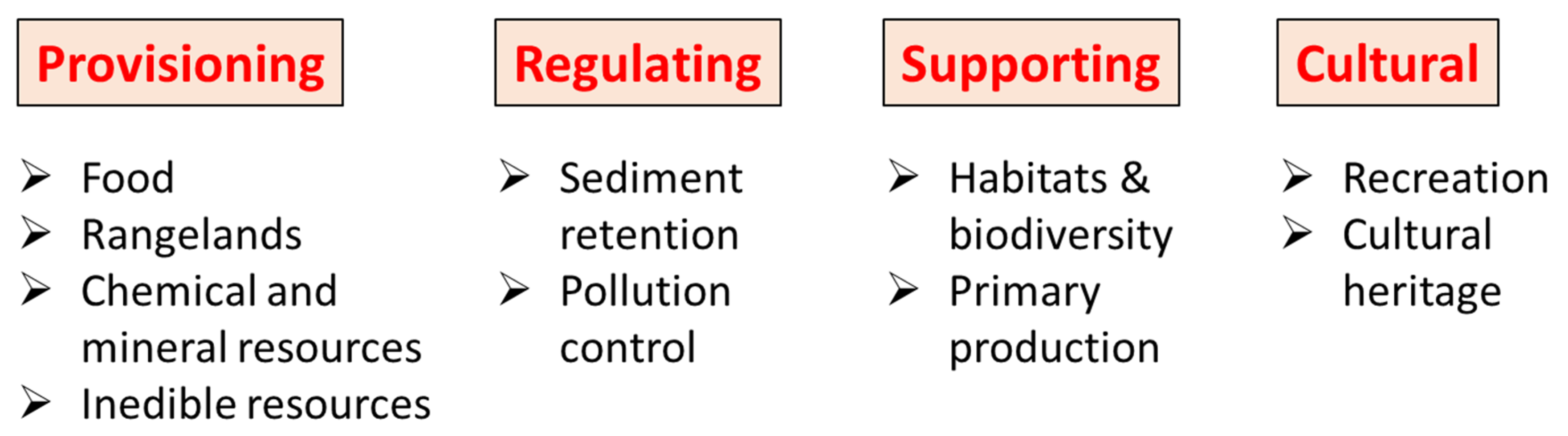
Ecosystem services are defined as goods and benefits that support human wellbeing as a result of the properties, functioning and dynamics of ecosystems [1,2,3,4,5]. Ecosystem services can be defined in several different ways, such as groups of conditions and processes that support human life [6,7], or with an emphasis on the different types of services provided by ecosystems (e.g., [7,8]) or in different environmental or human contexts [5,9,10]. Such debates around the definition of ecosystem services highlight the complexity of identifying, quantifying and then evaluating the benefits derived from these services. Broadly, ecosystem services can be categorized into four major types: provisioning, regulating, supporting and cultural [2,11,12] (Figure 1). Provisioning services such as food, water and fuel are potentially much easier to quantify and evaluate economically, and thus it is these factors that have been most commonly examined in previous studies (e.g., [11,13,14,15,16,17,18]). Cultural and regulating services are more difficult to identify and are less easily quantifiable [12,19,20].
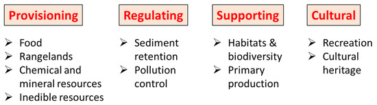
Figure 1.
General classification of ecosystem services (adapted from [11]).
The relationship between changes in ecosystem services and the most common forcing factors of land degradation, climate and land-use change has been undertaken in several studies using different methodological approaches. Field methods include measuring carbon storage within biomass and evaluating cultural services through ethnographic methods (e.g., [12,21,22,23]). Remote sensing methods include calculating ecosystem changes and normalized difference vegetation index (NDVI) values as a function of land degradation [18,24,25,26]. The advantage of remote sensing approaches is that changes over larger areas can be identified more easily, consistently and with the same resolution or error, which cannot be achieved in field studies, especially in remote locations. Thus, remote sensing has utility for identifying and mapping ecosystem service provision linked to ecosystem and land-use changes driven by regional-scale climate or ongoing land degradation [22,27,28].
In addition to evaluating changes in ecosystems and their services, various methods have also been used to convert ecosystem service provision to economic values [1,3,9,29,30,31,32]. The economic valuation elements that are specific to ecosystem service gain/loss are productivity loss, benefit transfer methods, replacement cost, avoidance cost, restoration cost and mitigation cost (e.g., [29,32,33]). This information can then be used for cost–benefit analysis to inform management decisions on ecosystem conservation or exploitation (e.g., [5,30,34,35]). The quantification of ecosystem services at a regional scale using ground surveys is problematic because it depends on the sampling strategy employed and the specific types of ecosystem services under examination, and systematic surveying in the field is time-consuming and expensive. Moreover, conversion of these services to economic values needs robust methods to be applied to minimize the economic valuation cost and provide a consistent methodology for continuous observation of the area under investigation [36,37].
Valuation of ecosystem service provision is particularly important under ongoing climate change and associated land degradation because these processes can significantly impact ecosystem properties and dynamics [38,39]. For example, land degradation may be considered as a decrease in net primary productivity (NPP) [14,40,41,42] and/or a reduction in the value of ecosystem and other environmental services (e.g., water, soil quality) [11,43]. Remote sensing methods of mapping regional vegetation change and land degradation have been widely used across southern Africa for examining spatial and temporal variations in semi-natural ecosystems that are important for biodiversity and ecosystem services (e.g., [22,26,27,28,44,45]). Specifically, NDVI values from time series of remote sensing data can be used to identify which regions are undergoing a decrease in NPP values [46,47] and are thus experiencing degradation, compared to those regions where NPP values are increasing (e.g., [48]). This in turn has implications for identifying sustainable development strategies for regions already experiencing climate stresses that impact on ecosystem vigor and ecosystem service provision [49,50,51,52]. A previous study on ecosystem service valuation in South Africa [53] used national GDP data in order to calculate the economic values of different ecosystem-dependent sectors, such as agriculture and tourism. This approach addresses only a narrow application of ecosystem services and does not look at the nature of the ecosystems themselves.
This study aimed to map and evaluate national- and regional-scale land-cover change and associated ecosystem services values across South Africa for the period 2001–2019 using MODIS satellite data. Changes in productivity of each land-cover class were used to calculate changes in economic values over time and space. Results of this study provide a first-order analysis of the economic values of ecosystem services in South Africa, which has not been done before at this scale using remote sensing data. This study further highlights the differences in aggregated values between different ecosystems as well as spatial variations at the province scale, which has not been previously done. This analysis provides a baseline for incorporation of ecosystem services as a fully valorized component of relevance to sustainable development strategies.
2. Materials and Methods
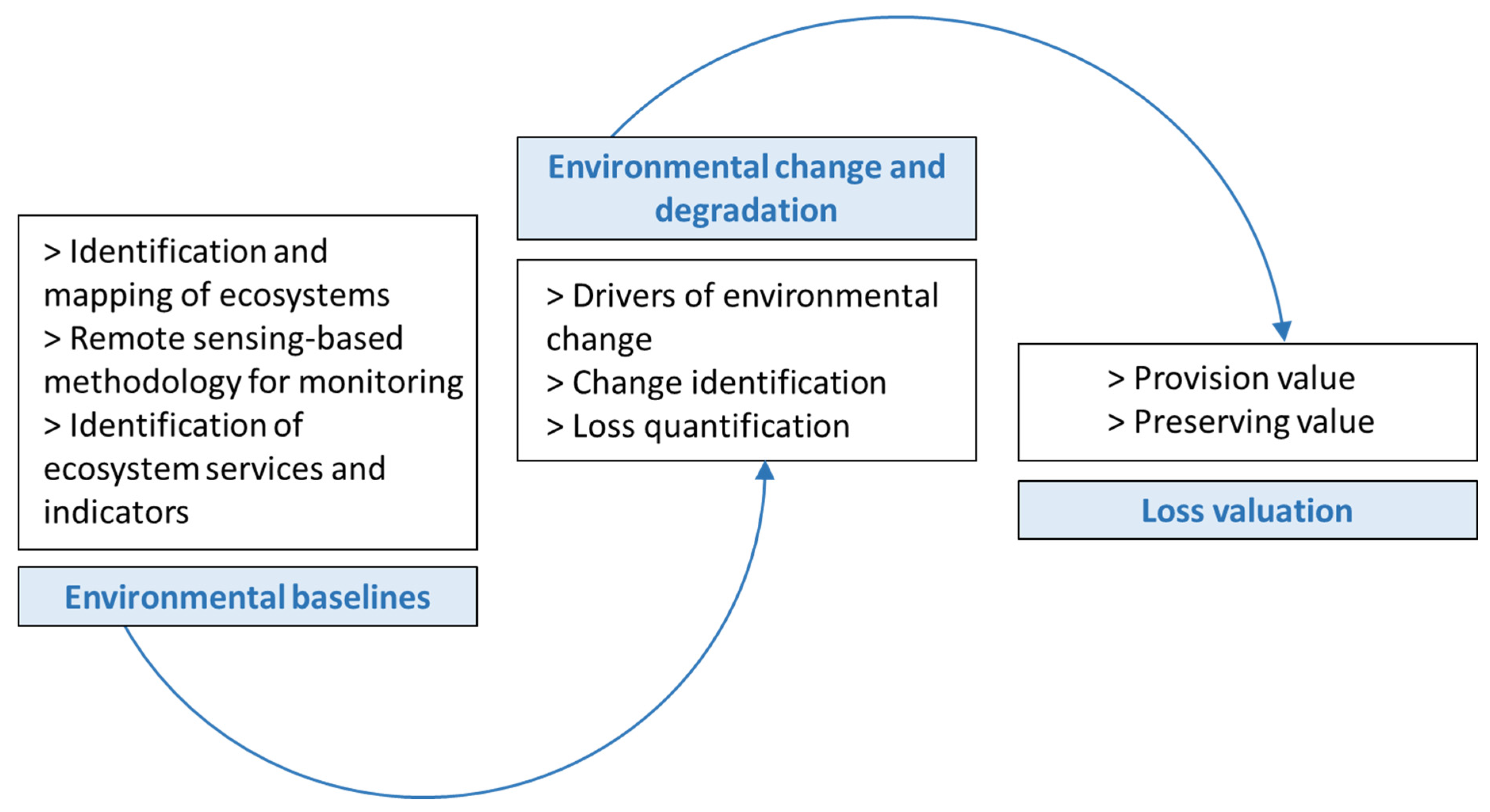
The general concept for valuation of ecosystem services is based on mapping of different ecosystems and land-cover classes, followed by quantification of ecosystem service values using values (in USD ha−1 yr−1) derived from the literature (Figure 2). MODIS remote sensing data were used in this study, with the time slices of 2001, 2005, 2010, 2014 and 2019. The MODIS data used were the MCD12Q1 MODIS/Terra + Aqua Land Cover product at 500 m spatial resolution (according to the classification of [54]). The MODIS data use 17 classes of land cover that include various natural vegetation types (11 classes), anthropogenically-altered land covers (3 classes) and non-vegetation land covers (3 classes). In this study, 15 classes were used in total. This is because some classes are not present in South Africa. Estimation of overall land degradation was calculated based on changes in NPP between each of the examined time slices (e.g., [55]).
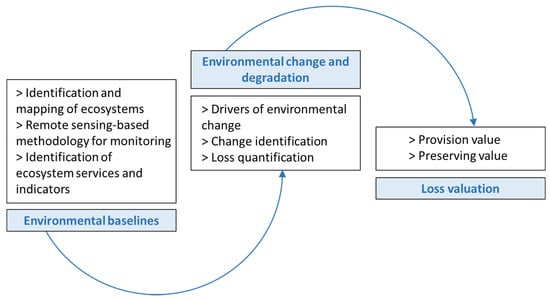
Figure 2.
Schematic diagram for the process of ecosystem services change and degradation (adapted from [11]).
The valuation of each land-cover class was estimated based on global published values for ecosystem services (e.g., [2,56]) as updated and summarized by [3] who integrated data from questionnaires and field workshops in various locations and from different ecosystems globally. Reference [3] (their Table 3) lists unit values in USD ha−1 yr−1 for different biome types for the years 1997 and 2011. Here, we used the averaged values for each biome to calculate ecosystem service values for the equivalent land-cover types from the MODIS data (Table 1). Many of these previous studies of land-cover valuation focused in particular on arid and semi-arid ecosystems and are thus relevant to land degradation studies in water-stressed locations such as South Africa. Previous use of MODIS data for calculating NPP shows statistically significant results [57], and this can frame the use of these data in this study as a direct indicator of land degradation. The NPP information was obtained from MODIS product at 500 m pixel resolution. The NPP values (in kg C m−2) were calculated based on the summation of the daily gross primary productivity (GPP) after subtracting the annual respirational factors [58]. The respirational factors were defined based on the characteristics of each biome using the Biome Properties Look-Up Table (BPLUT) (e.g., [59]). Four NPP product scenes were required to cover the South African terrestrial area for 2001, 2005, 2010, 2015 and 2019. The scenes were mosaicked and clipped using the national South African boundary layer.

Table 1.
Economic values (USD ha−1 yr−1) derived from [3], used in this study for calculation of total ecosystem service values per land-cover class.
Ecosystem degradation and its associated loss in economic value can be evaluated by assessing the net-value changes in various land-cover classes and changes in ecosystem service values from one class to another or degradation by loss of ecosystem service value taking place within the same class. The following equation was developed to estimate the value loss found in different ecosystems between different successive time slices:
where LDEL is land degradation economic loss, LCEV is land-cover economic value, and NPP is net primary productivity at j and j − 1 as current and previous time periods, respectively. The above equation has two parts: the potential ecosystem value and the degradation ratio. The latter corresponds to the ratio of changes in NPP values between two successive time slices. The equation can be further improved by including the land degradation index reported by [60] as the degradation part of the equation, although this was not done in this study for this first-order analysis.
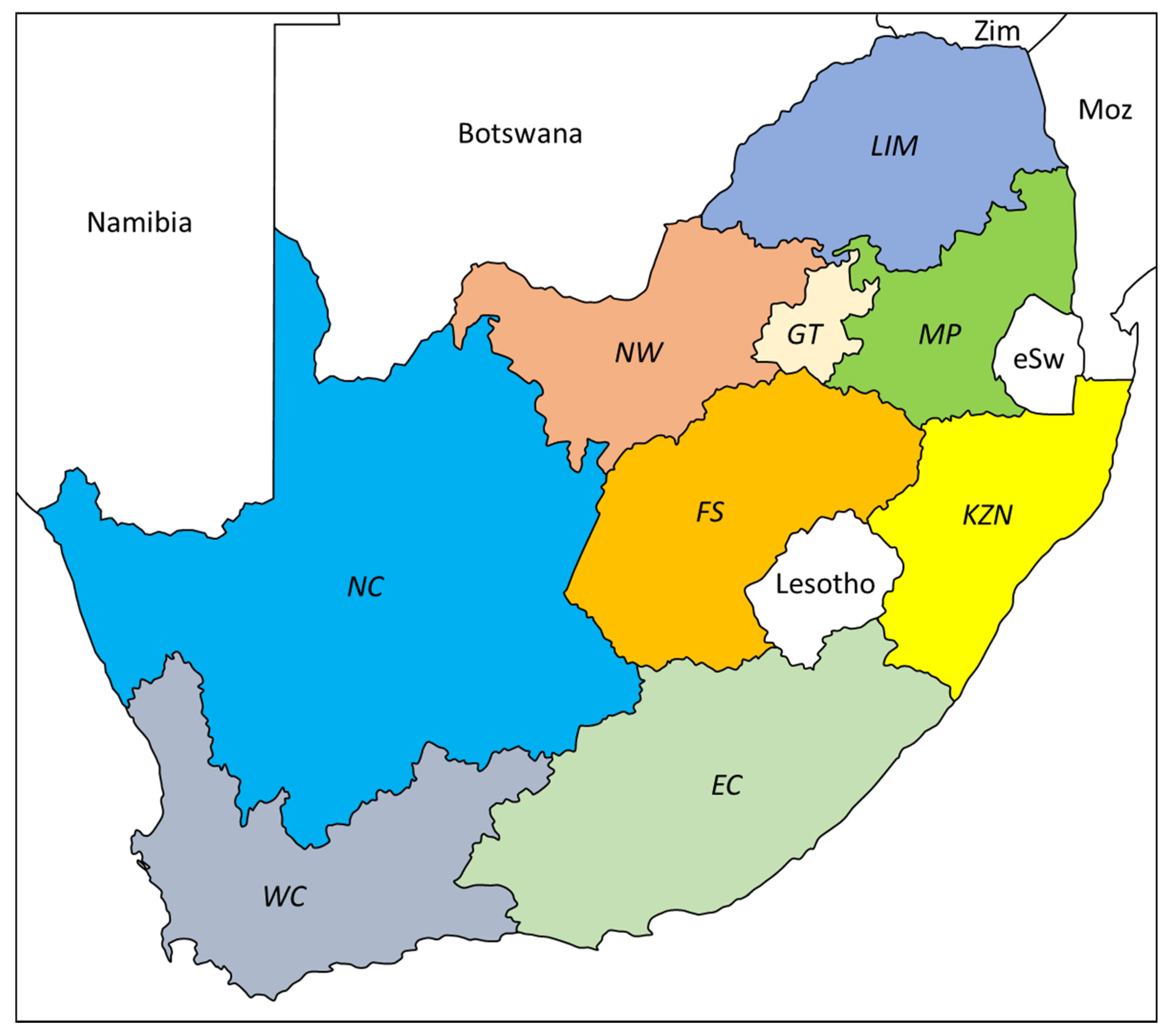
Spatially, analysis from MODIS data and from ecosystem service valuation was then considered at the scale of the nine individual provinces of South Africa (Figure 3) in order to examine the temporal variations of changes in land-cover type and ecosystem service values at a regional level.
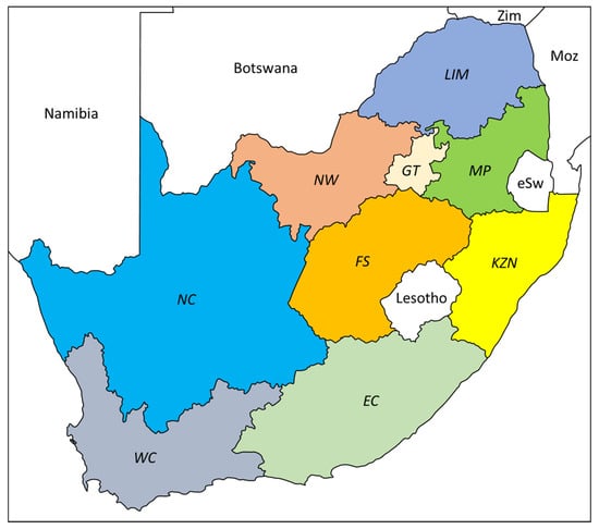
Figure 3.
Map of the nine provinces of South Africa which, from west to east, are: NC = Northern Cape, WC = Western Cape, NW = North West, FS = Free State, EC = Eastern Cape, KZN = KwaZulu-Natal, GT = Gauteng, MP = Mpumalanga, LIM = Limpopo. Also shown are Zim = Zimbabwe, Moz = Mozambique, eSW = eSwatini (Swaziland).
3. Results
3.1. Land-Cover Change
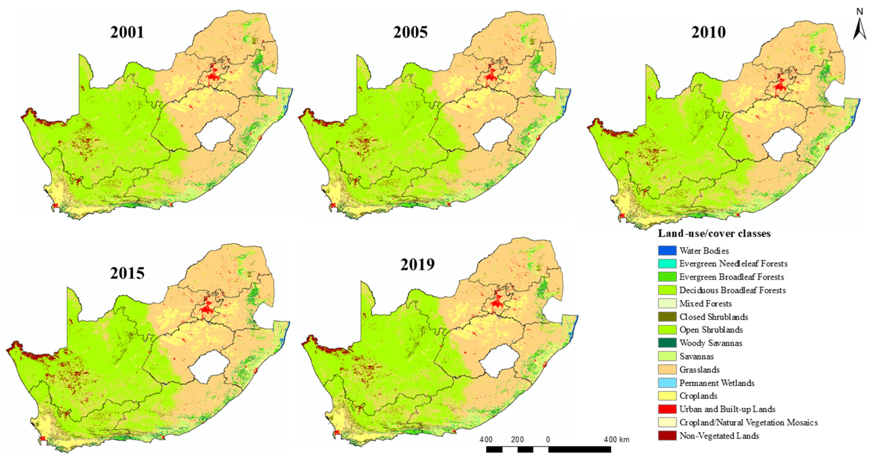
Classification of land cover using MODIS data in South Africa for the selected time slices is shown in Figure 4. MODIS class 3 (Deciduous Needleleaf Forests) is not included because this class does not appear in any year at either national or provincial level. Nationally, land cover is dominated by grasslands (average 45.3323%) and open shrublands (average 38.5289%) followed by croplands (average 5.3821%) and savanna (average 4.1185%) (Figure 5). Based on the classification of these land-cover classes at different time slices, trajectories of changes over time can be identified at a national scale (Table 2). Some classes (e.g., water bodies, savanna) show variability with no clear net changes, whereas other classes show more consistent patterns of increases (e.g., deciduous broadleaf forests, croplands) or decreases (e.g., evergreen broadleaf forests, grasslands). Land-cover values for 2015 may also reflect the strong El Niño event in that year, which impacted many different ecosystems in South Africa (e.g., [61]) because these events are associated with decreased regional rainfall and often drought conditions. Several broad patterns can be identified:
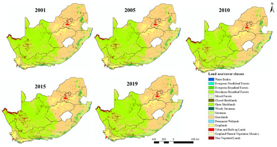
Figure 4.
Land-cover maps for South Africa for 2001, 2005, 2010, 2015 and 2019.
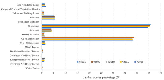
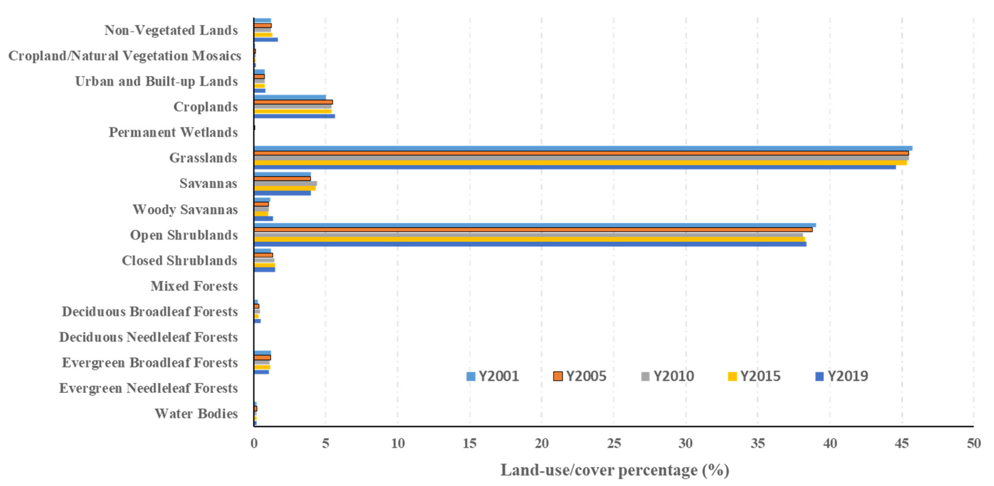
Figure 5.
Comparison between the percentage of land-cover classes at a national scale in 2001, 2005, 2010, 2015 and 2019.
Table 2.
Percentage land-cover types in South Africa for the time slices of analysis and interpretation of the overall trajectory of change: increase (up arrow), decrease (down arrow), NC = no change. Blank cells mean no clear picture of change.
- Water bodies show a declining trend throughout;
- Forests of different sorts increase;
- Open shrubland and grassland decrease;
- Croplands increase;
- Urban areas increase.
Despite these changes, variability between successive time slices of different land-cover types at a national scale has a range of only ±0.89–1.68%, yielding interannual values of ±0.16–0.42% but with an average of 0.24% (Figure 5). In detail, aggregated changes in land-cover type are reflected at a regional level, at the scale of individual provinces (Table 3), but these changes may be amplified because of the different proportions of certain land-cover classes that are present in different regions. For example, grasslands make up an average of 91.068% of the land area of Limpopo Province but only 13.581% in Northern Cape Province. This means that any changes in climatic or environmental conditions affecting grasslands would have the greatest impacts in the former and not the latter region. As a result, different provinces show different trajectories of change and with respect to specific land-cover types (Table 3).
Table 3.
Summary of trajectory of changes in the proportion of the land surface occupied by different ecosystem classes for different provinces of South Africa (shown in Figure 3) for the time period of analysis 2001–2019. Up arrow indicates a consistent increase in land area covered by that class; down arrow indicates a consistent decrease; NC = no change; NP = not present. Question mark indicates some variability in this general trend. Cells that are left blank indicate no consistent trend.
3.2. Changes in Net Primary Productivity as Proxy for Land Degradation
Values of NPP for the different years under analysis in kg C m−2 are presented in Figure 6 as an aggregated indicator for overall land degradation, as has been used in previous studies (e.g., [28,39,45,48,62]). It is notable that, at this national scale, similar patterns are seen in each time slice, reflecting the influence of summer rainfall (eastern side of South Africa), winter rainfall (western fringe of South Africa) and proximity to oceanic moisture sources [63,64]. This results in an inland precipitation gradient and an extensive area of low NPP values across Northern Cape Province. Thus, NPP values broadly reflect the rainfall climatology of the region.
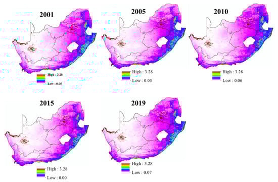
Figure 6.
Values of net primary productivity for the study area in 2001, 2005, 2010, 2015 and 2019, expressed as kg C m−2.
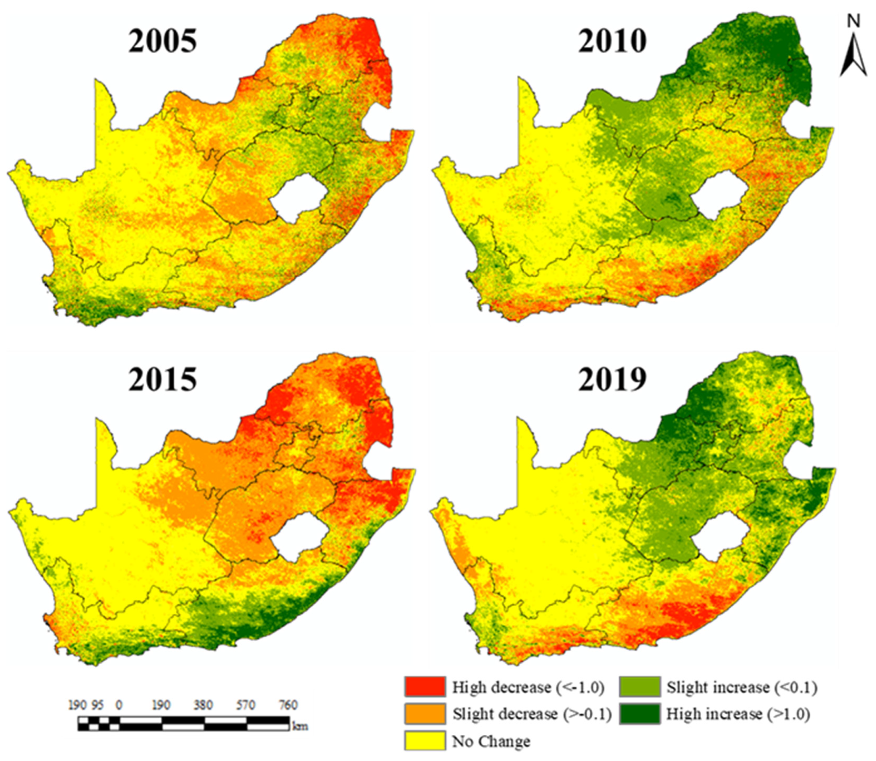
Comparison of NPP values for the different time slices shows similar patterns geographically but with some differences by time periods and for locations that are transitional between different ecosystems (Figure 6). There is greatest variability (both positive and negative) in eastern and southern peripheries adjacent to moisture sources. There is least variability in inland interiors. This can be seen in detail by considering changes in NPP values between successive time slices (Figure 7). This clearly shows that NPP values are consistent over time in the Northern Cape whereas there is an antiphase relationship between changes in NPP between northern/east-central areas (Limpopo, North West, Free State) and southern areas (Western Cape, Eastern Cape). This is likely to be a direct function of rainfall patterns [27].
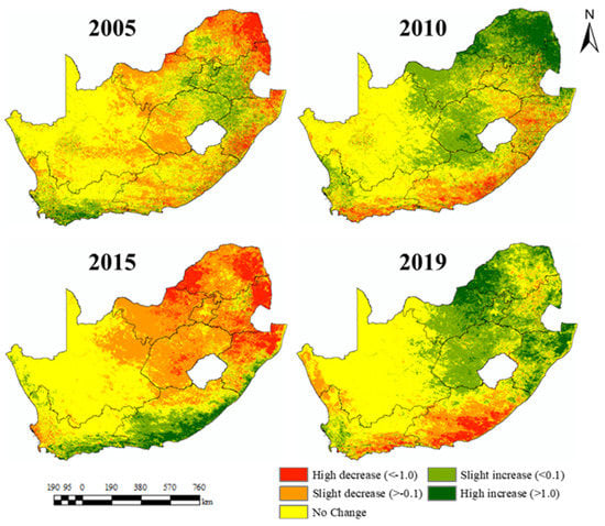
Figure 7.
Normalized difference between the NPP in different successive time periods (2001–2005, 2005–2010, 2010–2015, 2015–2019) in South Africa.
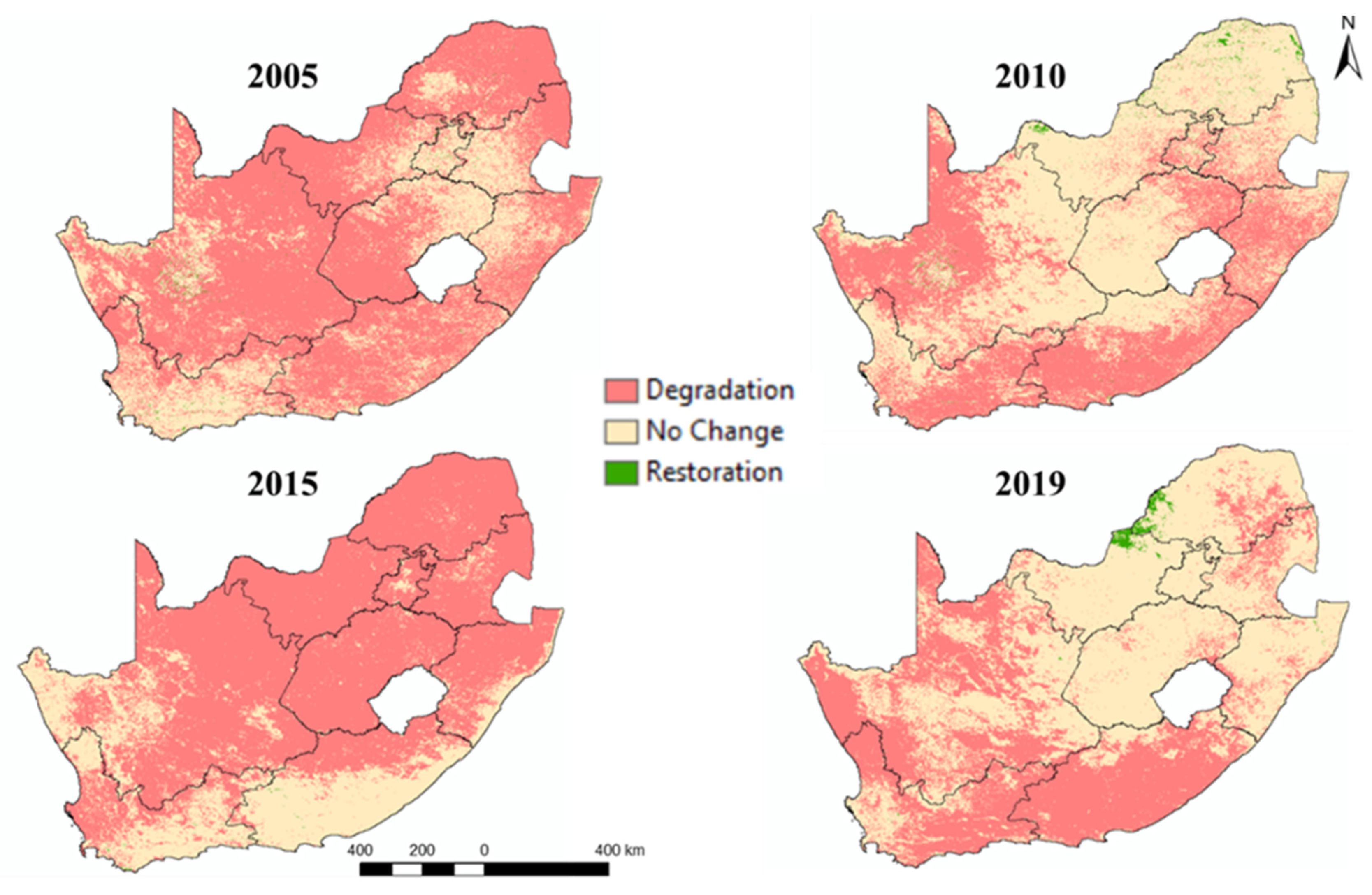
In detail, these data can be used to identify net patterns of land degradation (decrease in NPP) or restoration (increase in NPP) between successive time slices (Figure 8). These results show a consistent trajectory of land degradation in regions of Northern Cape, Western Cape and Eastern Cape. Other areas show some limited phases of degradation (Free State, North West, Limpopo) separated by periods of no change. There is also an antiphase relation between land degradation patterns between the 2010–2015 period and the preceding and subsequent periods, consistent with widespread aridity in 2015 (e.g., [65]).
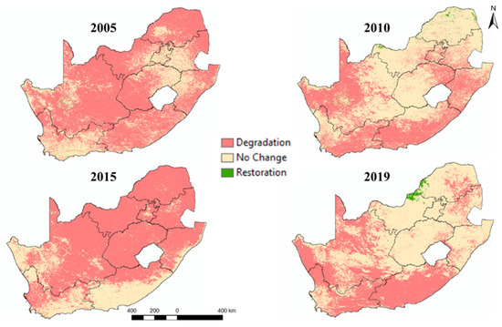
Figure 8.
Distribution of areas experiencing net degradation (NPP loss) and net restoration (NPP gain) according to normalized NPP values for different successive time periods (2001–2005, 2005–2010, 2010–2015, 2015–2019) in South Africa.
3.3. Valuation of Ecosystem Services Using Combined Approach of NPP and Land Cover
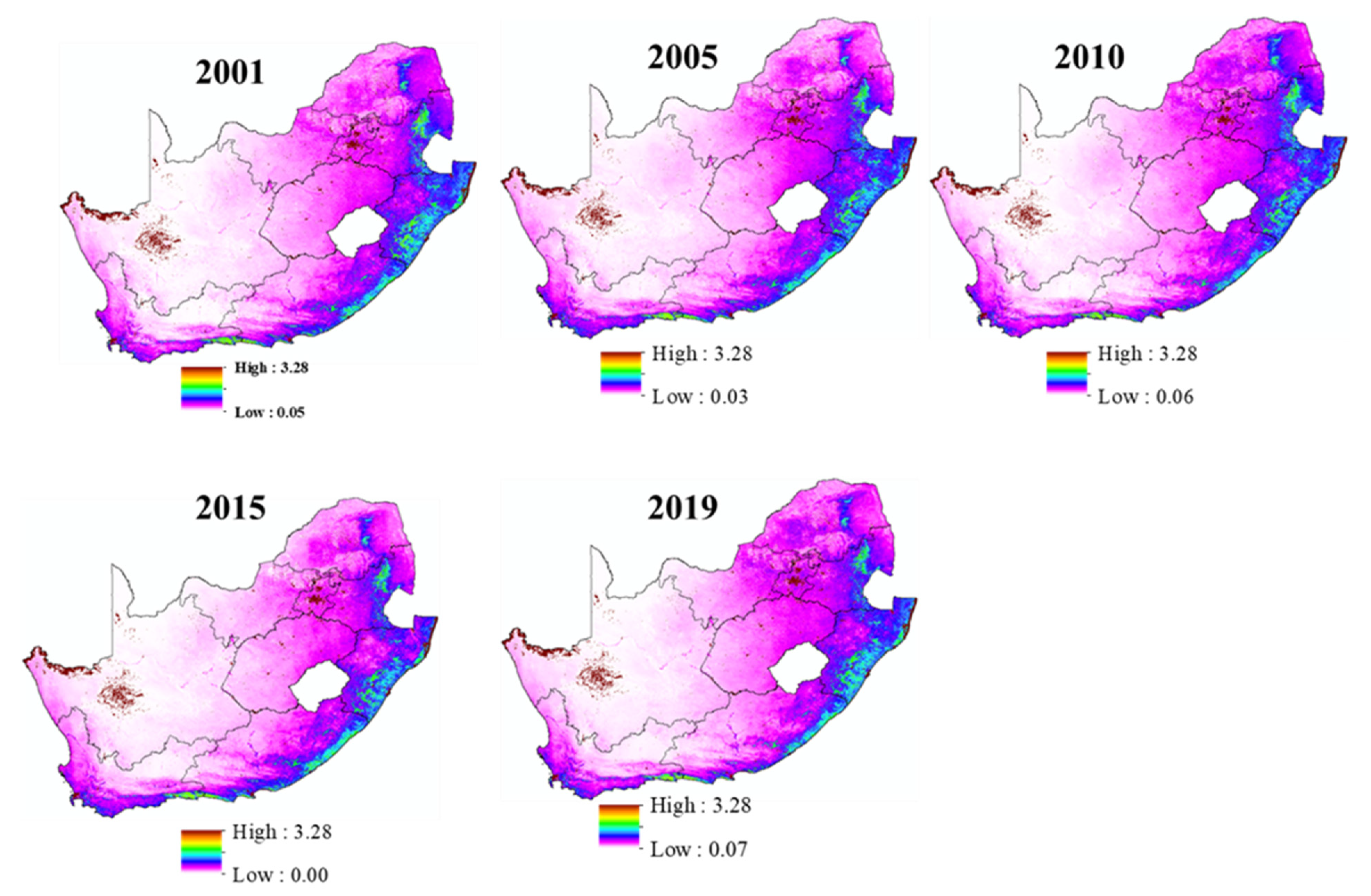
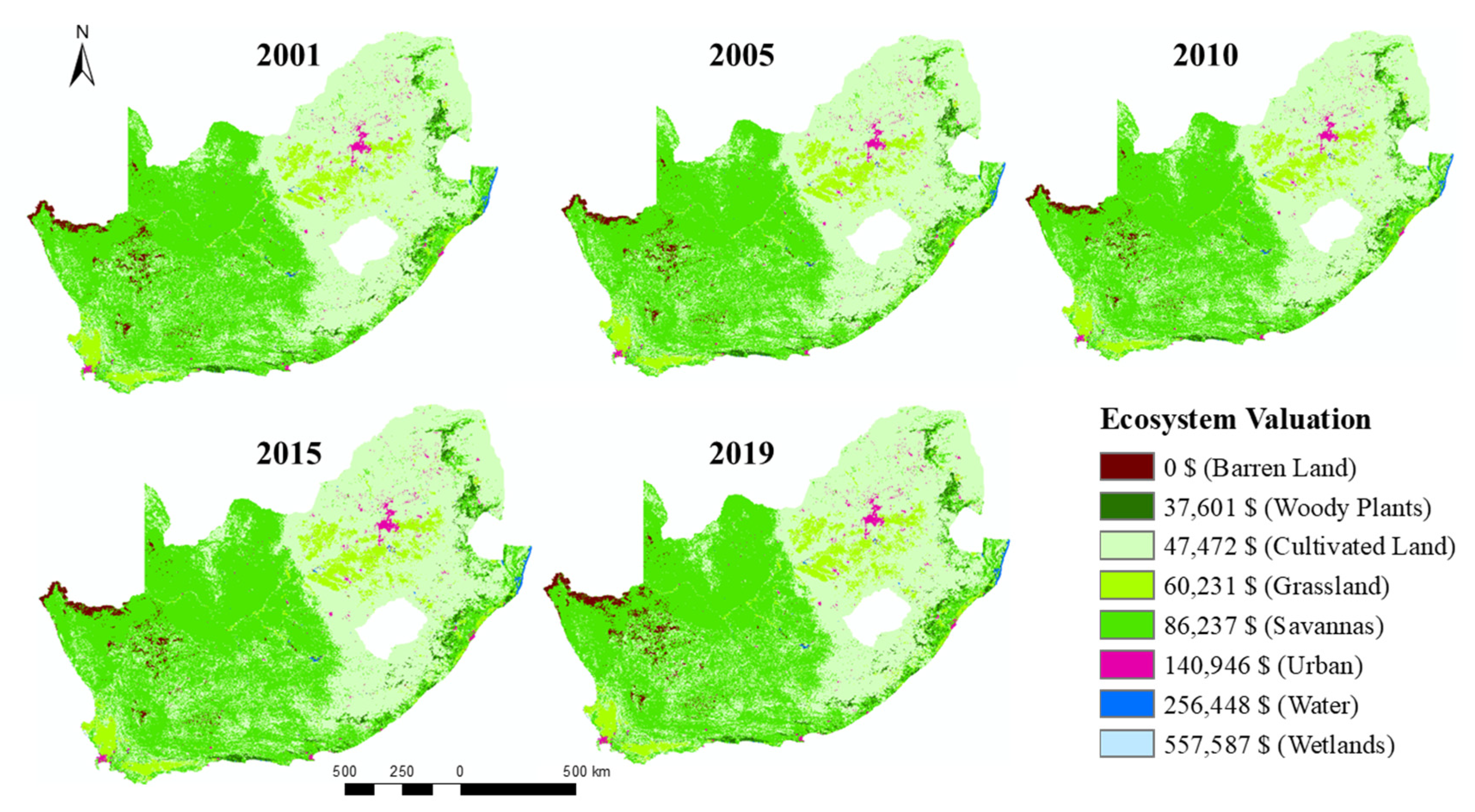
Equation (1) was used to calculate ecosystem service values based on global published values [3,14,56]. Results are presented in Table 4. This shows an annual value for ecosystem service provision in South Africa, averaged across the five time slices, of USD 437.727 billion. This compares with the national GDP (2019 values) of USD 351 billion; therefore ecosystem services represent some 125% of GDP. Table 4 also shows the different contributions to this national total by the different provinces. This ranges from the highest value in the Northern Cape (35.86% of total national ecosystem service values) to the lowest in Gauteng (1.45% of total national ecosystem service values). These two contrasting provinces, however, represent different end members of total contribution to GDP, with Northern Cape containing 2.15% of the national population and 2.19% of its GDP and Gauteng 25.82% of the national population and 34.94% of its GDP. This clearly shows—in these specific provinces—an opposite relationship between ecosystem service values and economic output values. (Other provinces show more similar values compared to Northern Cape and Gauteng.) The significance of this analysis is discussed below. Spatial patterns of ecosystem service values are shown in Figure 9. These show generally higher values in the west and lower in the east, consistent with spatial patterns of land-cover types (Figure 4). Smaller-scale and isolated patches of bare land and wetlands are also present, and these can be considered as anomalies set within broader landscape patterns.
Table 4.
Calculated annual values of ecosystem services (USD billion) by South African province and the national total for each time slice. Provinces are arranged from west to east as given in Figure 3. Comparison is also made between the % of total national ecosystem value for 2019, contained within each province, and the population of that province as a % of total national population (source: StatsSA, 2019). Population and ecosystem service values per province can also be compared with provincial contribution to GDP (2018 values) (available from https://www.southafricanmi.com/contribution-of-provinces-to-south-africa-gdp-9mar2020.html; accessed on 9 March 2020).
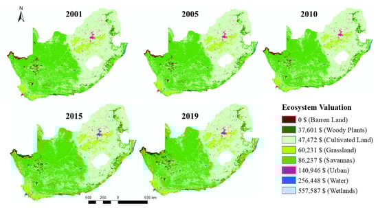
Figure 9.
Spatial patterns of economic valuation of ecosystem services (USD ha−1 yr−1) in South Africa for the years 2001, 2005, 2010, 2015 and 2019.
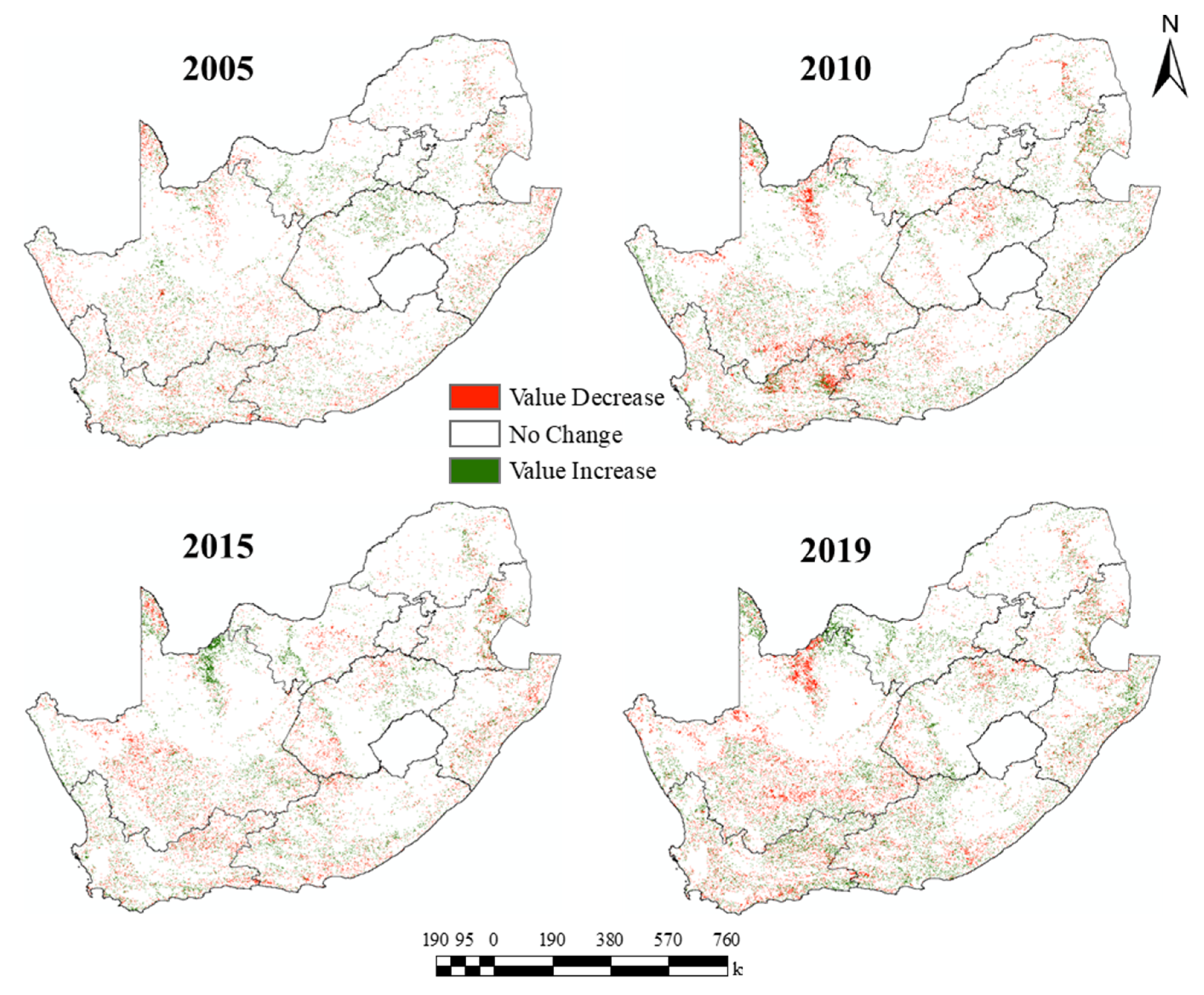
Comparison between successive time periods can be used to indicate where ecosystem service values are increasing or decreasing over time (Figure 10). These spatial patterns reflect climate-controlled transitions at ecological boundaries (ecotones), and this is therefore shown as linear zones across the landscape that reflect the spread/retreat of a particular land-cover type (e.g., [66]). This is seen particularly at the (east/west) grassland–woodland/savanna boundary.
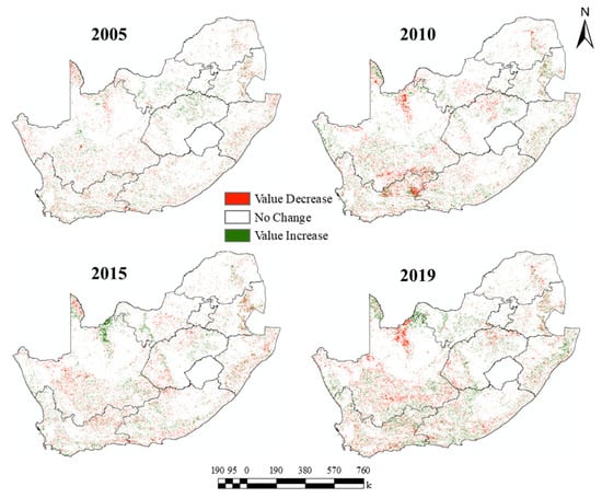
Figure 10.
Economic valuation of ecosystem services loss/gain for successive time periods (2001–2005, 2005–2010, 2010–2015, 2015–2019) in South Africa.
Comparison can therefore be made between spatial patterns of land degradation at each time increment (Figure 8) and how this translates into changes in ecosystem service values (Figure 10). This comparison shows that land degradation (decreased NPP) can take place in the absence of any change in land-cover type (i.e., where there is no change in ecosystem service values). However, if there is indeed land degradation related to reduced vegetation biomass and productivity, then this means that provisioning services of food and fiber are actually decreasing yet this is not reflected by any change in calculated ecosystem service values. This is a significant limitation in how ecosystem service values are calculated and the meaning and interpretation of these values.
4. Discussion
There are many studies on the responses of South African ecosystems to contemporary and future predicted climate change (e.g., [67,68,69,70,71]), but there is less understanding of how these responses affect the provision of different ecosystem services [72,73]. Likewise, many studies have examined ecosystem responses to land degradation (and its converse, restoration) in South Africa (e.g., [51,74,75,76]). In addition, any possible changes in species composition or the success of individual species within these mapped ecosystems, such as by the spread of invasive species, are also not well known (e.g., [77,78]). This issue is important because it has implications for the net values of services provided by these ecosystems or the balance of services of different types within ecosystems (Figure 1).
4.1. Land-Cover Changes and Their Implications
It is notable that some land-cover types show systematic positive or negative changes through the time period of analysis at national and provincial scales, whereas others do not (Table 2 and Table 3). Thus, different land-cover types show different sensitivities to climate forcing and/or land degradation and their different spatial and temporal patterns across the landscape that are reflected in ecosystem changes [24,46]. There is, in particular, covariability between woodland types, shrubland types and savanna types (Figure 4) driven by changes in tree density, and this can determine the outcome of the automated classification method used by MODIS. As a result, for these related classes, it is more useful to consider them as aggregated categories, reflecting the mosaic-like structure of woodlands in particular. For example, [79,80] showed that savanna grasslands across South Africa are presently experiencing increased invasive tree cover, causing a decrease in grassland biodiversity as well as decreased grassland ecosystem service provision such as grazing land. A decrease in these types of services may be offset or exceeded by an increase in other services provided by a developing tree cover such as fuel provision, microclimate or carbon sequestration. This shows that (1) autogenic changes in ecosystem properties can lead to significant changes in ecosystem services of different types, both positively and negatively (e.g., [73]), that are not captured by MODIS or similar classifications of ecosystem type, and that (2) NDVI is a useful first-order tool for evaluating ecosystem service availability, particularly provisioning services, because it reflects NPP and thus overall ecosystem vigor [57]. The rebalance between different land-cover types over time means that different ecosystem services and values also change. The absolute values of ecosystem service provision (Table 4) reflect only aggregated economic valuations. Changes in the commonness or rarity of certain ecosystem types have implications for the provision of certain types of services provided by certain ecosystems that may be concealed by statements of changes in total values [12,17,29]. In addition, absolute economic values also conceal the varied ways in which ecosystem services are provided according to their various categories (Figure 1). Thus, changes in the calculated area of certain land-cover types at a national scale do not necessarily map onto different ecosystem service types [5,18,36,51]. In addition, changes in land-cover types between individual provinces have implications for the local availability of certain types of ecosystem services that map across space. This may have implications for community availability and management of environmental resources at these local levels [81].
4.2. Valuation of Ecosystem Services
The results presented here (Table 4) for the first time calculate the economic value of different ecosystems’ services in South Africa. The general value of USD 437 billion (Table 4) is very different to the value of USD 17.68 billion calculated from a previous preliminary study of ecosystem services in South Africa by [53] who used historical (archival) datasets of land cover and calculated economic values on the basis of ecosystem contributions to GDP only. This methodology is very different to the approach adopted in this present study. Further, the results of this present study also show the complex regional-scale variations in these values that arise as a result of land-cover changes with associated changes in net service values per hectare (Table 4, Figure 10). However, these results of economic valuation do not reveal all ways in which ecosystem services can be exploited and thus valued from different perspectives (Figure 1). Economic valuations of non-provisioning services are more difficult to calculate because of the varied ways in which such resources are used, including for indirect or cultural services [7,12,23,24,81]. The high values cited in the literature for some types of land-cover classes (Table 1) may falsely imply that certain land covers are more important economically for human activity or wellbeing than others. Different agricultural ecosystems are not directly considered in this scheme despite their key role in direct food production, and neither does this scheme consider the other varied ways in which economic value can be derived apart from food and fiber production. The link between ecosystem service values and their direct contribution to human livelihoods and wellbeing are thus not well understood [17,30,82] or built into models of service valuation [9,17].
The opposite relationship between ecosystem service values and GDP contribution in Northern Cape and Gauteng (Table 4) shows that, in both these cases, the economic basis of these provinces is not linked to ecosystem service provision. The areal extent of different land-cover classes (biomes) within a region also has complex relationships to ecosystem service value. For example, the increased extent of a certain land cover increases its commonness and decreases its rarity and vice versa. Thus, land-cover types may be more valuable if they are rarer or more isolated in a landscape or if they are located in an area of high population density. This situation has been described in the case of xeric grasslands on koppies (hills) in the city of Johannesburg (Gauteng) where these hills host 71% of the province’s endemic species [83]. A single numerical evaluation of ecosystem service provision, therefore, fails to capture the complexity or multifaceted nature of an ecosystem in the landscape or the varied ways in which human activity intersects with, exploits or values such ecosystems [17,29,36].
4.3. Implications for Climate Change, Land Degradation and Sustainable Development
This study, in evaluating ecosystem services at a national scale using remote sensing methods, provides a consistent and standardized methodology that can be used across different spatial scales and in different contexts. Further, repeat surveys can be used to quantify losses or gains in ecosystem service values over time, which provide a baseline for evaluating the impacts of climate change and land degradation on ecosystem values, properties and biodiversity [18,22,23]. In this study, evidence for changes in land-cover types over decadal time scales and regional spatial scales reflects the impacts of climate change and not local-scale factors such as land management [71,77,80]. Future climate projections can therefore be used to predict future regional ecological patterns at these regional scales (e.g., [70,78]). We show that changes in ecosystem distributions have implications for land degradation trends (Figure 8) and patterns of increased/decreased ecosystem service values (Table 4, Figure 10). These in turn have implications for strategies toward sustainable development, managing negative impacts of climate change on different ecosystems and their service provision to local communities and wider issues of maintaining biodiversity and reducing soil erosion, amongst others [20,51,81]. This is important because some ecosystems can maintain their existing services or even enhance their future service provision under appropriate management strategies [5,26].
5. Conclusions
Natural resources are precious local to global assets, and ecosystem service evaluation is one means of quantifying the potential value of these assets. This study provides the first national-scale evaluation of ecosystem services in South Africa, using a remote sensing methodology that can be applied to other areas and contexts. The calculated total ecosystem service value is USD 437 billion, which is ~125% of GDP. There is significant spatial variation across the country in terms of the regions where the highest and lowest values are found, which has implications for potential resource availability for use by local communities and in the context of sustainable regional development. This highlights the potential for untapped ecosystem services to be exploited as a tool for sustainable development strategies. Although provisioning services can be calculated based on ecosystem properties and NPP alone, other ecosystem services such as cultural services cannot be easily calculated in the same way. This means that different approaches must be undertaken in order to characterize the real, functional values that any ecosystem has in the landscape. This is a future research priority in order to ensure both sustainability of ecosystem properties and functions and for rural socioeconomic development and human wellbeing.
Author Contributions
The funded project was coordinated by M.A.M.A.E., and work was additionally undertaken by G.L., M.M.A.-Z. and R.H. J.K. wrote this paper in collaboration with M.A.M.A.E. with the other authors commenting and approving the submitted paper. All authors have read and agreed to the published version of the manuscript.
Funding
The Department of Environmental Affairs (South Africa) and the joint National Research Foundation (NRF) of South Africa and the National Natural Science Foundation of China (NSFC) project funded this research work (No. NSFC170315224611).
Institutional Review Board Statement
Not applicable.
Informed Consent Statement
Not applicable.
Data Availability Statement
Data available on request.
Acknowledgments
We thank two reviewers for their comments on this paper.
Conflicts of Interest
The authors declare no conflict of interest.
References
- Costanza, R.; D’Arge, R.; de Groot, R.; Farber, S.; Grasso, M.; Hannon, B.; Limburg, K.; Naeem, S.; O’Neill, R.V.; Paruelo, J.; et al. The value of the world’s ecosystem services and natural capital. Nature 1997, 387, 253–260. [Google Scholar] [CrossRef]
- Costanza, R.; Kubiszewski, I.; Ervin, D.; Bluffstone, R.; Boyd, J.; Brown, D.; Chang, H.; Dujon, V.; Granek, E.; Polasky, S.; et al. Valuing ecological systems and services. F1000 Biol. Rep. 2011, 3, 14. [Google Scholar] [CrossRef] [Green Version]
- Costanza, R.; de Groot, R.; Sutton, P.; van der Ploeg, S.; Anderson, S.J.; Kubiszewski, I.; Farber, S.; Turner, R.K. Changes in the global value of ecosystem services. Glob. Environ. Chang. 2014, 26, 152–158. [Google Scholar] [CrossRef]
- Walters, C.J.; Christensen, V.; Martell, S.J.; Kitchell, J.F. Possible ecosystem impacts of applying MSY policies from single-species assessment. ICES J. Mar. Sci. 2005, 62, 558–568. [Google Scholar] [CrossRef] [Green Version]
- Egoh, B.; Reyers, B.; Rouget, M.; Richardson, D.M.; Le Maitre, D.C.; van Jaarsveld, A.S. Mapping ecosystem services for planning and management. Agric. Ecosyst. Environ. 2008, 127, 135–140. [Google Scholar] [CrossRef]
- Daily, G.C.; Matson, P.A.; Vitousek, P.M. Ecosystem services supplied by soil. In Nature’s Services: Societal Dependence on Natural Ecosystems; Daily, G., Ed.; Island Press: Washington, DC, USA, 1997; pp. 113–132. [Google Scholar]
- Jackson, S.; Palmer, L.R. Reconceptualizing ecosystem services: Possibilities for cultivating and valuing the ethics and practices of care. Progr. Hum. Geogr. 2015, 39, 122–145. [Google Scholar] [CrossRef] [Green Version]
- Grimmond, S.; Bouchet, V.; Molina, L.T.; Baklanov, A.; Tan, J.; Schlünzen, K.H.; Mills, G.; Golding, B.; Masson, V.; Ren, C.; et al. Integrated urban hydrometeorological, climate and environmental services: Concept, methodology and key messages. Urban Clim. 2020, 33, 100623. [Google Scholar] [CrossRef]
- Gómez-Baggethun, E.; Ruiz-Pérez, M. Economic valuation and the commodification of ecosystem services. Progr. Phys. Geogr. 2011, 35, 613–628. [Google Scholar] [CrossRef] [Green Version]
- Van Noordwijk, M.; Leimona, B.; Jindal, R.; Villamor, G.B.; Vardhan, M.; Namirembe, S.; Catacutan, D.; Kerr, J.; Minang, P.A.; Tomich, T.P. Payments for environmental services: Evolution toward efficient and fair incentives for multifunctional landscapes. Ann. Rev. Environ. Res. 2012, 37, 389–420. [Google Scholar] [CrossRef]
- MEA [Millennium Ecosystems Assessment]. Ecosystems and Human Well-being: Synthesis; Island Press: Washington, DC, USA, 2005. [Google Scholar]
- Sen, S.; Guchhait, S.K. Urban green space in India: Perception of cultural ecosystem services and psychology of situatedness and connectedness. Ecol. Indic. 2021, 123, 107338. [Google Scholar] [CrossRef]
- Smiraglia, D.; Ceccarelli, T.; Bajocco, S.; Salvati, L.; Perini, L. Linking trajectories of land change, land degradation processes and ecosystem services. Environ. Res. 2016, 147, 590–600. [Google Scholar] [CrossRef] [PubMed]
- Sutton, P.; Anderson, S.; Costanza, R.; Kubiszewski, I. The ecological economics of land degradation: Impacts on ecosystem service values. Ecol. Econ. 2016, 129, 182–192. [Google Scholar] [CrossRef]
- Tarrasón, D.; Ravera, F.; Reed, M.S.; Dougill, A.J.; Gonzalez, L. Land degradation assessment through an ecosystem services lens: Integrating knowledge and methods in pastoral semi-arid systems. J. Arid Environ. 2016, 124, 205–213. [Google Scholar] [CrossRef]
- Turner, K.G.; Anderson, S.; Gonzales-Chang, M.; Costanza, R.; Courville, S.; Dalgaard, T.; Dominati, E.; Kubiszewski, I.; Ogilvy, S.; Porfirio, L.; et al. A review of methods, data, and models to assess changes in the value of ecosystem services from land degradation and restoration. Ecol. Modell. 2016, 319, 190–207. [Google Scholar] [CrossRef]
- Boerema, A.; Rebelo, A.J.; Bodi, M.B.; Esler, K.J.; Meire, P. Are ecosystem services adequately quantified? J. Appl. Ecol. 2017, 54, 358–370. [Google Scholar] [CrossRef]
- Cerretelli, S.; Poggio, L.; Gimona, A.; Yakob, G.; Boke, S.; Habte, M.; Coull, M.; Peressotti, A.; Black, H. Spatial assessment of land degradation through key ecosystem services: The role of globally available data. Sci. Total Environ. 2018, 628–629, 539–555. [Google Scholar] [CrossRef]
- Dhanya, B.; Sathish, B.N.; Viswanath, S.; Purushothaman, S. Ecosystem services of native trees: Experiences from two traditional agroforestry systems in Karnataka, Southern India. Int. J. Biodiv. Sci. Ecosyst. Serv. Manag. 2014, 10, 101–111. [Google Scholar] [CrossRef]
- Schild, J.E.M.; Vermaat, J.E.; de Groot, R.S.; Quatrini, S.; van Bodegom, P.M. A global meta-analysis on the monetary valuation of dryland ecosystem services: The role of socio-economic, environmental and methodological indicators. Ecosyst. Serv. 2018, 32, 78–89. [Google Scholar] [CrossRef] [Green Version]
- Rieprich, R.; Schnegg, M. The value of landscapes in northern Namibia: A system of intertwined material and nonmaterial services. Soc. Nat. Res. 2015, 28, 941–958. [Google Scholar] [CrossRef] [Green Version]
- Del Río-Mena, T.; Willemen, L.; Tesfamariam, G.T.; Beukes, O.; Nelson, A. Remote sensing for mapping ecosystem services to support evaluation of ecological restoration interventions in an arid landscape. Ecol. Indic. 2020, 113, 106182. [Google Scholar] [CrossRef]
- Mowat, S.; Rhodes, B. Identifying and assigning values to the intangible cultural benefits of ecosystem services to traditional communities in South Africa. S. Afr. J. Sci. 2020, 116, 6970. [Google Scholar] [CrossRef]
- Van Jaarsveld, A.S.; Biggs, R.; Scholes, R.J.; Bohensky, E.; Reyers, B.; Lynam, T.; Musvoto, C.; Fabricius, C. Measuring conditions and trends in ecosystem services at multiple scales: The Southern African Millennium Ecosystem Assessment (SAfMA) experience. Philos. Trans. R. Soc. Ser. B 2005, 360, 425–441. [Google Scholar] [CrossRef] [PubMed] [Green Version]
- Huang, X.; Han, X.; Ma, S.; Lin, T.; Gong, J. Monitoring ecosystem service change in the City of Shenzhen by the use of high-resolution remotely sensed imagery and deep learning. Land Degrad. Dev. 2019, 30, 1490–1501. [Google Scholar] [CrossRef]
- Nyamekye, C.; Schönbrodt-Stitt, S.; Amekudzi, L.K.; Zoungrana, B.J.-B.; Thiel, M. Usage of MODIS NDVI to evaluate the effect of soil and water conservation measures on vegetation in Burkina Faso. Land Degrad. Dev. 2021, 32, 7–19. [Google Scholar] [CrossRef]
- Wessels, K.J.; Prince, S.D.; Malherbe, J.; Small, J.; Frost, P.E.; VanZyl, D. Can human-induced land degradation be distinguished from the effects of rainfall variability? A case study in South Africa. J. Arid Environ. 2007, 68, 271–297. [Google Scholar] [CrossRef]
- Harris, A.; Carr, A.S.; Dash, J. Remote sensing of vegetation cover dynamics and resilience across southern Africa. Int. J. Appl. Earth Obs. Geoinform. 2014, 28, 131–139. [Google Scholar] [CrossRef]
- Christie, M.; Fazey, I.; Cooper, R.; Hyde, T.; Kenter, J.O. An evaluation of monetary and non-monetary techniques for assessing the importance of biodiversity and ecosystem services to people in countries with developing economies. Ecol. Econ. 2012, 83, 67–78. [Google Scholar] [CrossRef]
- Dikgang, J.; Muchapondwa, E. Local communities’ valuation of environmental amenities around the Kgalagadi Transfrontier Park in Southern Africa. J. Environ. Econ. Pol. 2017, 6, 168–182. [Google Scholar] [CrossRef]
- Browne, M.; Fraser, G.; Snowball, J. Economic evaluation of wetland restoration: A systematic review of the literature. Restor. Ecol. 2018, 26, 1120–1126. [Google Scholar] [CrossRef]
- Baba, C.A.K.; Hack, J. Economic valuation of ecosystem services for the sustainable management of agropastoral dams. A case study of the Sakabansi dam, northern Benin. Ecol. Indic. 2019, 107, 105648. [Google Scholar] [CrossRef]
- Möller, A.; Ranke, U. Estimation of the on-farm-costs of soil erosion in Sleman, Indonesia. WIT Trans. Ecol. Environ. 2006, 89, 43–52. [Google Scholar]
- Lele, S. Watershed services of tropical forests: From hydrology to economic valuation to integrated analysis. Curr. Opin. Environ. Sustain. 2009, 1, 148–155. [Google Scholar] [CrossRef]
- De Wit, M.; Zyl, H.; Crookes, D.; Blignaut, J.; Jayiya, T.; Goiset, V.; Mahumani, B. Including the economic value of well-functioning urban ecosystems in financial decisions: Evidence from a process in Cape Town. Ecosyst. Serv. 2012, 2, 38–44. [Google Scholar] [CrossRef]
- O’Farrell, P.J.; De Lange, W.J.; Le Maitre, D.C.; Reyers, B.; Blignaut, J.N.; Milton, S.J.; Atkinson, D.; Egoh, B.; Maherry, A.; Colvin, C.; et al. The possibilities and pitfalls presented by a pragmatic approach to ecosystem service valuation in an arid biodiversity hotspot. J. Arid Environ. 2011, 75, 612–623. [Google Scholar] [CrossRef] [Green Version]
- Favretto, N.; Luedeling, E.; Stringer, L.C.; Dougill, A.J. Valuing ecosystem services in semi-arid rangelands through stochastic simulation. Land Degrad. Dev. 2017, 28, 65–73. [Google Scholar] [CrossRef]
- Tully, K.; Sullivan, C.; Weil, R.; Sanchez, P. The State of Soil Degradation in Sub-Saharan Africa: Baselines, Trajectories, and Solutions. Sustainability 2015, 7, 6523–6552. [Google Scholar] [CrossRef] [Green Version]
- Matarira, D.; Mutanga, O.; Dube, T. Landscape scale land degradation mapping in the semi-arid areas of the Save catchment, Zimbabwe. S. Afr. Geogr. J. 2021, 103, 183–203. [Google Scholar] [CrossRef]
- Vitousek, P.M.; Ehrlich, P.R.; Ehrlich, A.H.; Matson, P.A. Human appropriation of the products of photosynthesis. BioScience 1986, 36, 368–373. [Google Scholar] [CrossRef]
- Rojstaczer, S.; Sterling, S.M.; Moore, N.J. Human appropriation of photosynthesis products. Science 2001, 294, 2549–2552. [Google Scholar] [CrossRef]
- Le, Q.B.; Nkonya, E.; Mirzabaev, A. Biomass Productivity-Based Mapping of Global Land Degradation Hotspots; ZEF Discussion Papers on Development Policy 193; ZEF: Bonn, Germany, 2014. [Google Scholar]
- Von Braun, J.; Gerber, N.; Mirzabaev, A.; Nkonya, E. The Economics of Land Degradation; ZEF Working Paper Series 109; ZEF: Bonn, Germany, 2013. [Google Scholar]
- Dubovyk, O. The role of Remote Sensing in land degradation assessments: Opportunities and challenges. Eur. J. Remote Sens. 2017, 50, 601–613. [Google Scholar] [CrossRef]
- Venter, Z.S.; Scott, S.L.; Desmet, P.G.; Hoffman, M.T. Application of Landsat-derived vegetation trends over South Africa: Potential for monitoring land degradation and restoration. Ecol. Indic. 2020, 113, 106206. [Google Scholar] [CrossRef]
- Ardö, J. Comparison between remote sensing and a dynamic vegetation model for estimating terrestrial primary production of Africa. Carb. Bal. Manag. 2015, 10, 8. [Google Scholar] [CrossRef] [PubMed] [Green Version]
- Pan, S.; Dangal, S.R.S.; Tao, B.; Yang, J.; Tian, H. Recent patterns of terrestrial net primary production in Africa influenced by multiple environmental changes. Ecosyst. Health Sustain. 2015, 1, 18. [Google Scholar] [CrossRef] [Green Version]
- Higginbottom, T.P.; Symeonakis, E. Identifying Ecosystem Function Shifts in Africa Using Breakpoint Analysis of Long-Term NDVI and RUE Data. Remote Sens. 2020, 12, 1894. [Google Scholar] [CrossRef]
- Clover, J.; Eriksen, S. The effects of land tenure change on sustainability: Human security and environmental change in southern African savannas. Environ. Sci. Pol. 2009, 12, 53–70. [Google Scholar] [CrossRef]
- Andersson, E.; Brogaard, S.; Olsson, L. The Political Ecology of Land Degradation. Ann. Rev. Environ. Res. 2021, 36, 295–319. [Google Scholar] [CrossRef]
- Sigwela, A.; Elbakidze, M.; Powell, M.; Angelstam, P. Defining core areas of ecological infrastructure to secure rural livelihoods in South Africa. Ecosyst. Serv. 2017, 27, 272–280. [Google Scholar] [CrossRef]
- Smith, P.; Calvin, K.; Nkem, J.; Campbell, D.; Cherubini, F.; Grassi, G.; Korotkov, V.; Le Hoang, A.; Lwasa, S.; McElwee, P.; et al. Which practices co-deliver food security, climate change mitigation and adaptation, and combat land degradation and desertification? Glob. Chang. Biol. 2020, 26, 1532–1575. [Google Scholar] [CrossRef] [PubMed] [Green Version]
- Turpie, J.K.; Forsythe, K.J.; Knowles, A.; Blignaut, J.; Letley, G. Mapping and valuation of South Africa’s ecosystem services: A local perspective. Ecosyst. Serv. 2017, 27, 179–192. [Google Scholar] [CrossRef]
- Sulla-Menashe, D.; Gray, J.M.; Abercrombie, S.P.; Friedl, M.A. Hierarchical mapping of annual global land cover 2001 to present: The MODIS Collection 6 Land Cover product. Remote Sens. Environ. 2019, 222, 183–194. [Google Scholar] [CrossRef]
- Running, S.; Mu, Q.; Zhao, M. MYD17A3H MODIS/Aqua Net Primary Production Yearly L4 Global 500m SIN Grid V006 [Dataset]. NASA EOSDIS Land Processes DAAC. Available online: https://lpdaac.usgs.gov/products/myd17a3hv006/ (accessed on 21 January 2015). [CrossRef]
- De Groot, R.S.; Wilson, M.A.; Boumans, R.M.J. A typology for the classification, description and valuation of ecosystem functions, goods and services. Ecol. Econ. 2002, 41, 393–408. [Google Scholar] [CrossRef] [Green Version]
- Pachavo, G.; Murwira, A. Remote sensing net primary productivity (NPP) estimation with theaid of GIS modelled shortwave radiation (SWR) in a Southern African Savanna. Int. J. Appl. Earth Obs. Geoinform. 2014, 30, 217–226. [Google Scholar] [CrossRef]
- Running, S.W.; Zhao, M. Daily GPP and Annual NPP (MOD17A2H/A3H) and Year-end Gap-Filled (MOD17A2HGF/A3HGF) Products NASA Earth Observing System MODIS Land Algorithm. Available online: https://lpdaac.usgs.gov/documents/495/MOD17_User_Guide_V6.pdf (accessed on 28 February 2021).
- Cheng, B.-Y.; Zhang, Q.; Lyapustin, A.I.; Wang, Y.; Middleton, E.M. Impacts of light use efficiency and fPAR parameterization on gross primary production modelling. Agric. Forest Meteorol. 2014, 189–190, 187–197. [Google Scholar] [CrossRef]
- Tswai, D.R.; Malherbe, J.; Dekker, C.; Mashimbye, Z.E.; Van den Berg, E.C.; Nyamugama, A.; Elbasit, M.A.M.; Chirima, J.G.; Nell, J.P.; Nkambule, V.T. Phase 1 of Desertification, Land Degradation and Drought (DLDD) land cover mapping impact indicator of the United Nations Convention to Combat Desertification (UNCCD); DEA: Pretoria, South Africa, 2016.
- Xulu, S.; Peerbhay, K.; Gebreslasie, M.; Ismail, R. Unsupervised Clustering of Forest Response to Drought Stress in Zululand Region, South Africa. Forests 2019, 10, 531. [Google Scholar] [CrossRef] [Green Version]
- Wessels, K.J.; van den Bergh, F.; Scholes, R.J. Limits to detectability of land degradation by trend analysis of vegetation index data. Remote Sens. Environ. 2012, 125, 10–22. [Google Scholar] [CrossRef]
- Jury, M.R. Climate trends in southern Africa. S. Afr. J. Sci. 2013, 109, 980. [Google Scholar] [CrossRef] [Green Version]
- Favre, A.; Philippon, N.; Pohl, B.; Kalognomou, E.-A.; Lennard, C.; Hewitson, B.; Nikulin, G.; Dosio, A.; Panitz, H.-J.; Cerezo-Mota, R. Spatial distribution of precipitation annual cycles over South Africa in 10 CORDEX regional climate model present-day simulations. Clim. Dyn. 2016, 46, 1799–1818. [Google Scholar] [CrossRef]
- Kolusu, S.R.; Shamsudduha, M.; Todd, M.C.; Taylor, R.G.; Seddon, D.; Kashaigili, J.J.; Ebrahim, G.Y.; Cuthbert, M.O.; Sorensen, J.P.R.; Villholth, K.G.; et al. The El Niño event of 2015–2016: Climate anomalies and their impact on groundwater resources in East and Southern Africa. Hydrol. Earth Syst. Sci. 2019, 23, 1751–1762. [Google Scholar] [CrossRef] [Green Version]
- Rouget, M.; Cowling, R.M.; Pressey, R.L.; Richardson, D.M. Identifying spatial components of ecological and evolutionary processes for regional conservation planning in the Cape Floristic Region, South Africa. Divers. Distrib. 2003, 9, 191–210. [Google Scholar] [CrossRef]
- Midgley, G.F.; Hannah, L.; Millar, D.; Thuiller, W.; Booth, A. Developing regional and species-level assessments of climate change impacts on biodiversity in the Cape Floristic Region. Biol. Conserv. 2003, 112, 87–97. [Google Scholar] [CrossRef]
- Masubelele, M.L.; Hoffman, M.T.; Bond, W.J.; Gambiza, J. A 50 year study shows grass cover has increased in shrublands of semi-arid South Africa. J. Arid Environ. 2014, 104, 43–51. [Google Scholar] [CrossRef]
- Stevens, N.; Erasmus, B.F.N.; Archibald, S.; Bond, W.J. Woody encroachment over 70 years in South African savannahs: Overgrazing, global change or extinction aftershock? Philos. Trans. R. Soc. Ser. B 2016, 371, 20150437. [Google Scholar] [CrossRef] [PubMed] [Green Version]
- Lawal, S.; Lennard, C.; Hewitson, B. Response of southern African vegetation to climate change at 1.5 and 2.0° global warming above the pre-industrial level. Clim. Serv. 2019, 16, 100134. [Google Scholar] [CrossRef]
- Skowno, A.L.; Jewitt, D.; Slingsby, J.A. Rates and patterns of habitat loss across South Africa’s vegetation biomes. S. Afr. J. Sci. 2021, 117, 8182. [Google Scholar] [CrossRef]
- Turpie, J.K. The existence value of biodiversity in South Africa: How interest, experience, knowledge, income and perceived level of threat influence local willingness to pay. Ecol. Econ. 2003, 46, 199–216. [Google Scholar] [CrossRef]
- Chisholm, R.A. Trade-offs between ecosystem services: Water and carbon in a biodiversity hotspot. Ecol. Econ. 2010, 69, 1973–1987. [Google Scholar] [CrossRef]
- Bourne, A.; Muller, H.; de Villiers, A.; Alam, M.; Hole, D. Assessing the efficiency and effectiveness of rangeland restoration in Namaqualand, South Africa. Plant Ecol. 2017, 218, 7–22. [Google Scholar] [CrossRef]
- Willemen, L.; Crossman, N.D.; Quatrini, S.; Egoh, B.; Kalaba, F.K.; Mbilinyi, B.; de Groot, R. Identifying ecosystem service hotspots for targeting land degradation neutrality investments in south-eastern Africa. J. Arid Environ. 2018, 159, 75–86. [Google Scholar] [CrossRef]
- Crookes, D.J.; Blignaut, J.N. Investing in natural capital and national security: A comparative review of restoration projects in South Africa. Heliyon 2019, 5, e01765. [Google Scholar] [CrossRef] [Green Version]
- Young, A.J.; Guo, D.; Desmet, P.G.; Midgley, G.F. Biodiversity and climate change: Risks to dwarf succulents in Southern Africa. J. Arid Environ. 2016, 129, 16–24. [Google Scholar] [CrossRef]
- Bezeng, B.S.; Yessoufou, K.; Taylor, P.J.; Tesfamichael, S.G. Expected spatial patterns of alien woody plants in South Africa’s protected areas under current scenario of climate change. Sci. Rep. 2020, 10, 7038. [Google Scholar] [CrossRef] [PubMed]
- Skowno, A.L.; Thompson, M.W.; Hiestermann, J.; Ripley, B.; West, A.G.; Bond, W.J. Woodland expansion in South African grassy biomes based on satellite observations (1990–2013): General patterns and potential drivers. Glob. Chang. Biol. 2017, 23, 2358–2369. [Google Scholar] [CrossRef] [PubMed]
- Scheiter, S.; Gaillard, C.; Martens, C.; Erasmus, B.F.N.; Pfeiffer, M. How vulnerable are ecosystems in the Limpopo province to climate change? S. Afr. J. Bot. 2018, 116, 86–95. [Google Scholar] [CrossRef]
- Knight, J. Environmental services: A new approach towards addressing Sustainable Development Goals in sub-Saharan Africa. Front. Sustain. Food Syst. 2021, 5, 687863. [Google Scholar] [CrossRef]
- Cilliers, S.; Cilliers, J.; Lubbe, R.; Siebert, S. Ecosystem services of urban green spaces in African countries—Perspectives and challenges. Urban Ecosyst. 2013, 16, 681–702. [Google Scholar] [CrossRef]
- Pfab, M. The quartzite ridges of Gauteng. Veld Flora 2002, 88, 56–59. [Google Scholar]
Publisher’s Note: MDPI stays neutral with regard to jurisdictional claims in published maps and institutional affiliations. |
© 2021 by the authors. Licensee MDPI, Basel, Switzerland. This article is an open access article distributed under the terms and conditions of the Creative Commons Attribution (CC BY) license (https://creativecommons.org/licenses/by/4.0/).