Research on Sustainable Land Use Based on Production–Living–Ecological Function: A Case Study of Hubei Province, China

Abstract

After decades of rapid development, there exists insufficient and contradictory land use in the world, and social, economic and ecological sustainable development is facing severe challenges. Balanced land use functions (LUFs) can promote sustainable land use and reduces land pressures from limited land resources. In this study, we propose a new conceptual index system using the entropy weight method, regional center of gravity theory, coupling coordination degree model and obstacle factor identification model for LUFs assessment and spatial-temporal analysis. This framework was applied to 17 cities in central China’s Hubei Province using 39 indicators in terms of production–living–ecology analysis during 1996–2016. The result shows that (1) LUFs showed an overall upward trend during the study period, while the way of promotion varied with different dimensions. Production function (PF) experienced a continuous enhancement during the study period. Living function (LF) was similar in this aspect, but showed a faster rising tendency. EF continued to increase during 1996–2011, but declined during 2011–2016. LUFs were higher in the east than in the west, and slightly higher in the south than in the north. The spatial coordination was enhanced during the study period. (2) The overall level of coupling coordination degree continued to increase during 1996–2016, while regional difference declined obviously, indicating a good developing trend. However, the absolute level was still not satisfactory. (3) The obstacle degree of PF was always dominant, and LF showed a downward trend, while EF showed an increasing trend. Benefit index (A2), Comfort index (B2) and Green index (C1) constituted the primary obstacle factor for each dimension. Added-value of high and new technology industry (A2-3) and land use intensity (A3-2) were key factors restricting PF. Number of medical practitioner (B1-4) and internet penetration rate (B2-3) were key factors restricting LF. Air quality rate (C3-1) and wetland coverage rate (C1-4) were key factors restricting EF. This study can help to give a more detailed understanding of sustainable land use for the particularity of China from a land function perspective and provide lessons and suggestions for other developing countries in the world.

1. Introduction

The world we live in is complex while policy makers and scientists prefer to reduce complexity for the purpose of simplifying decision-making. However, reducing assessment to a single dimension may miss cross-linkages and eventually lead to poor decision-making [1]. Land is a comprehensive system which is composed of economic, social and ecological subsystems [2,3] and it is also the material basis and fountain of resources for the country’s social and economic development, the place and environment for national survival and various activities. Mankind uses it for a multitude of purposes, and for striving for sustainable development.

Land use functions (LUFs) are defined as the private and public goods and services provided by different land uses that summarize the most relevant economic, environmental and social issues of a region [4], which was stimulated by the European project named “Sustainability Impact Assessment: Tools for Environmental Social and Effects of Multifunctional Land Use in Europe Regions (SENSOR)”. According to LUFs, land systems can be categorized into three classes (Figure 1): production land (PL), living land (LL) and ecological land (EL), namely, production–living–ecological land (PLEL) [5,6].

According to the above figure, PL provides agricultural products, industrial products and service products as the leading function of the region, ensuring the survival and development of mankind. LL carries and maintains human settlements, mainly exerts the function of human habitation, consumption, leisure and entertainment. EL refers to the main function of providing ecological products and ecological services, playing an extremely important role in maintaining, regulating and safeguarding regional ecology. In short, PL is regarded as driving force, EL is foundation, LL is considered as the link of PLEL. The three aspects of PLEL are closely related and mutually transformed [7]. Due to the population explosion and inadequate land resources, the competitions among PLEL are becoming increasingly fierce. The long-lasting and rapid urbanization has led to the rapid expansion of construction land (LL), and a large number of cultivated land (PL) and ecological land (EL) around the town have been occupied [8]. Likewise, forest land and water bodies (EL) have been occupied by cultivated land (PL) for food production. There exist insufficient and contradictory situations during land use and social, economic and ecological sustainable development is facing severe challenges.

Actually, land use competitions are the results of conflicts and compromises with different functions and relevant underlying objectives [9,10]. Contemporary people have started to realize that a piece of land not only provides economic production function, but also provides social and ecological functions [11]. PLEL exerts their dominant functions respectively. Moreover, PLEL also exerts their non-principal functions. As a result, functional superposition and multi-functions occur (Figure 2). Multifunctional land use aims at maximizing the benefits obtained from a given parcel of land [12]. Gradually, land use management has changed the way from focusing on one single function to multi-functional land use. Therefore, multifunctional land use has become an important path to solving these conflicts and promoting efficient and sustainable land use [13].

Researches of multifunctional land use concepts that originated from the agricultural sector, referring to the simultaneous provision of diverse output and the consequent satisfaction of multiple demands [14,15,16,17]. Then, researches extended from agriculture to economy, society and environment, as well as sustainable land use assessment [18,19,20], attracting widespread attentions from scientists and policy makers. To balance the three dimensions (economic, social and environmental) of sustainability, SENSOR project proposed a conceptual framework of regional sustainability assessment from the perspective of LUFs [4]. Each sustainability dimension is represented by three LUFs: Economic (Residential and Industrial Services, Land-based Production, Infrastructure), Social (Work, Health and Recreation, Culture) and Environmental (Abiotic Resources, Provision of Habitat, Ecosystem Processes), giving nine land use functions in all. The SENSOR project greatly promoted the application of multifunctional land use methodology in the field of land use sustainability impact assessment. Scholars established a conceptual framework to assess Chinese LUFs during 1985–2005 [21]. Then, policy scenarios and detailed subdivisions of land utilization were taken into account by scholars [22]. Further, a methodological framework was presented based on the concept of LUFs to assess the impact of land use policies on sustainable development in developing countries [23]. However, despite the increase in publications on LUFs, more research might be completed on the connotation of sustainable land use [24].

Since the reform and opening up, China’s land space utilization has made remarkable achievements with relatively scarce land resource endowments [8,25]. The Report on the Government’s Work at the Fourth Session of the Twelfth National People’s Congress on 5 March 2016 emphasized that the objectives of land use in China should focus on integrated development for production, living, and ecology. Further, Commission of the European Community in the Impact Assessment Guidelines also stated that sustainable impact assessment should perform an integration of economic, environmental and social issues. Therefore, the purpose of land use is to pursue coordination of LUFs and realize sustainable land use. Thus, this paper proposed a conceptual index system for sustainable land use assessment in terms of the three aspects of LUFs of production–living–ecology. Then, this paper demonstrated the use of proposed LUFs assessment index system in 17 cities of Hubei Province in China as an example using entropy weight method, regional center of gravity theory, coupling coordination degree model and obstacle factor identification model. The results confirmed the situation that there is still a long way to go for the sustainable land use in China, and measures should be taken to realize the scientific development that emphasizes multi-dimensional coordination and overall progress. This paper is committed to promoting balanced LUFs, insisting that only comprehensive coordinated development of LUFs is the sustainable land use. Compared with the past research, this study can help to give a more detailed understanding of sustainable land use for the particularity of China and provide lessons and suggestions for other developing countries in the world.

2. Materials and Methods

2.1. Study Area and Data Source

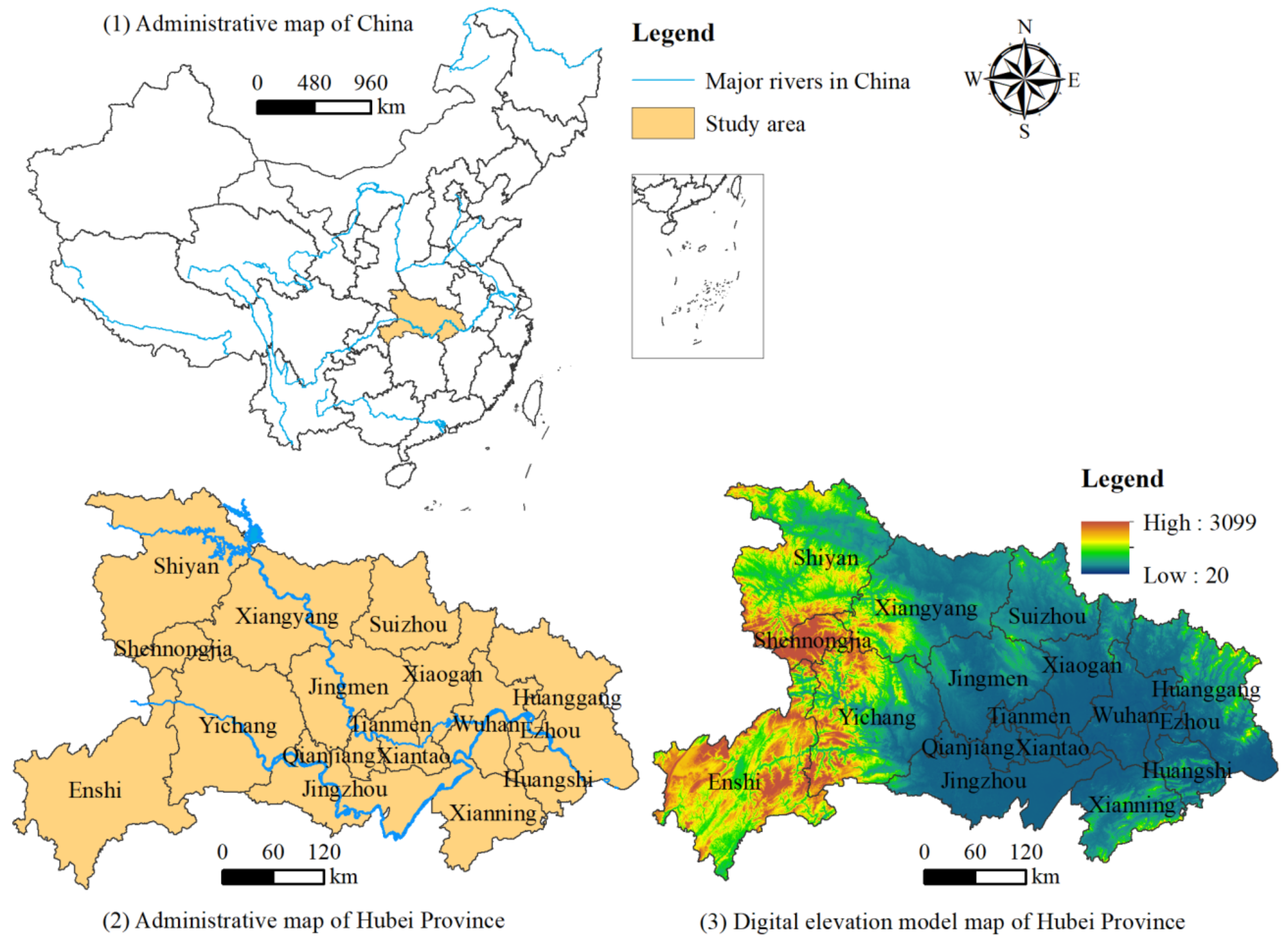
2.1.1. Study Area

Hubei Province (HP) is located in the central region of China, between the northern latitude of 29°01′53″–33°6′47″ and the east longitude of 108°21′42″–116°07′50″. HP has various types of landforms, including mountains, hills, plains and lake areas with outstanding natural endowment advantages. The terrain of HP is roughly surrounded by mountains in the east, west and north, low in the middle, showing the incomplete basin slightly open to the south. There are 17 municipal administrative districts in HP (Figure 3).

As an important implementation area of China’s central rise strategy, HP has achieved rapid progress of urbanization and industrialization in recent years, its economic status in the country has been rising, and its comprehensive strength in regional development has been significantly improved. In 2019, HP’s regional gross domestic product (GDP) reached 4.58 trillion RMB, ranking 7/31 in China (except Hong Kong, Macao and Taiwan). The province’s urbanization rate reached 61.00%, higher than the national average (60.60%). The ecological environment quality of HP is generally good, and the river water, lake water, reservoir water, air quality and the level of urban environmental noise show a good trend. Therefore, it is of great practical significance to choose HP as a research area to conduct the study, and the case has a high reference value for other regions.

2.1.2. Data Sources and Data Pre-Processing

Data in this study mainly included land use data and statistics data of economic, demographic, environmental and social development. Land use data were collected from Resource and Environment Data Cloud Platform (http://www.resdc.cn/), while specific statistics data were mainly derived from the Hubei Statistical Yearbook, Hubei Rural Statistics Yearbook, China Urban Statistics Yearbook and China Urban Construction Statistics Yearbook. Further, it was supplemented by the regional statistical yearbook of the 17 cities (states, forest areas). At the same time, work reports and statistical bulletins of the Hubei provincial government and municipal governments, the statistics reports of the Natural Resources Department, Ecological Environment Department and other relevant departments were used to make up for the missing data in yearbooks.

Data of different indicators may have different units and characteristics. Therefore, in order to eliminate the influence of dimension, magnitude, and positive and negative orientation, the numeric data needs pre-processing before using [26]. A standardization method of the data range was used to pre-process the original data. After the transformation, all the indicators’ values were transformed into normalized values with a numerical range from 0 to 1.

$$X_i^{\prime }=\left\{\begin{array}{cc}\left(X_i-X_{min}\right)/\left(X_{max}-X_{min}\right)& \left(positiveindicator\right)\\ \left(X_{max}-X_i\right)/\left(X_{max}-X_{min}\right)& \left(negative indicator\right)\end{array}\right.$$

(1)

where $X_i^{\prime }$ means the normalized value. $X_i$ refers to the original value. $X_{max}$ and $X_{min}$ are the maximum and minimum values, respectively.

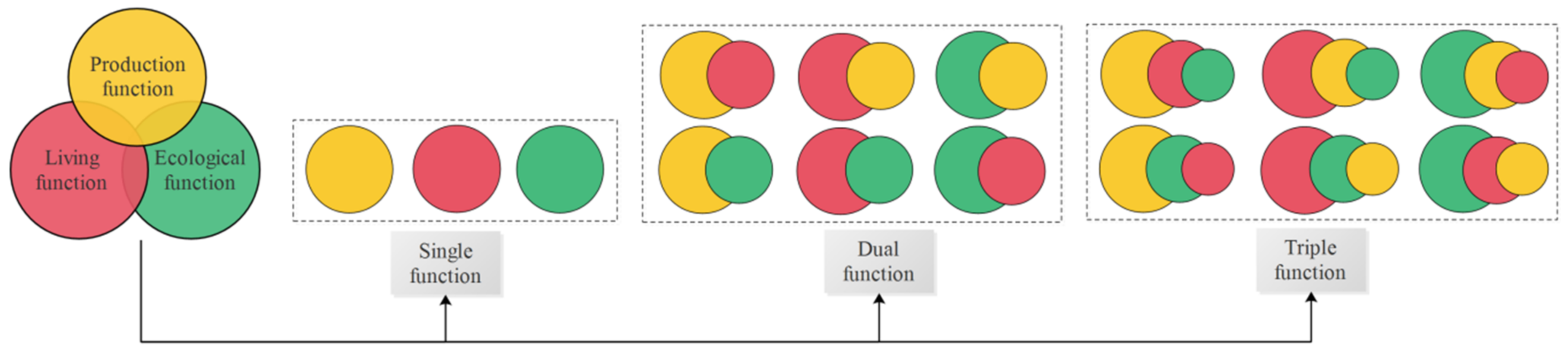
2.2. Construction of Three-Dimensional Indicator System

Firstly, this study fully analyzed the connotation of sustainable land use based on LUFs. Secondly, this research compared and analyzed the evaluation indicators in relevant researches [27], then an initial evaluation indicator system was established. Thirdly, the initial indicator system was sent to 20 experts and scholars in the fields of land resource management, natural geography, regional development and planning for argumentation. The rules of argumentation were as follows. (1) If more than half of the experts consider an indicator to be unimportant or inappropriate, the indicator is eliminated. (2) If the correlation between the indicators is considered strong, the indicators are grouped or the indicator whose data are easily obtained is chosen. (3) The experts can also propose new indicators to be added to the existing indicator system and accept the next round of expert argumentation. (4) After three rounds of expert argumentation, indicators that more than 80% of the experts identified are included in the final indicator system. The final indicator system is shown in

Table 1. Evaluation indicator system and weight of land space utilization.

Level 1 Indicators	Level 2 Indicators	Level 3 Indicators	Units	Weight
Production function A	Input index (A1)	A1-1 Investment of fixed assets per unit of construction land area (+)	100 million RMB/km2	0.0413
		A1-2 Employment in secondary and tertiary industry per unit of construction land area (+)	person/km2	0.0419
		A1-3 Input intensity of R&D Expenditure (+)	%	0.0355
		A1-4 Mechanical power of per unit of arable land area (+)	kW/hectare	0.0108
		A1-5 Primary production laborers per unit of arable land area (+)	person/hectare	0.0127
	Benefit index (A2)	A2-1 Fiscal revenue per unit of construction land area (+)	10,000 RMB/km2	0.0419
		A2-2 GDP of secondary and tertiary industry per unit of construction land area (+)	100 million RMB/km2	0.0496
		A2-3 Added-value of high and new technology industry per unit of land area (+)	100 million RMB/km2	0.0851
		A2-4 Added-value of primary industry per unit of arable land area (+)	10,000 RMB/hectare	0.0092
		A2-5 Yield per unit of sown area (+)	ton/hectare	0.0123
	Intensity index (A3)	A3-1 Construction land area per capita (+)	m2	0.0378
		A3-2 Development intensity of land space (+)	%	0.0533
		A3-3 Multiple cropping index (+)	dimensionless	0.019
		A3-4 Effective irrigation index (+)	dimensionless	0.0253
Living function B	Basic living index (B1)	B1-1 Drinking water penetration rate (+)	%	0.0103
		B1-2 Fuel gas penetration rate (+)	%	0.0061
		B1-3 Engel’s coefficient of urban family (−)	dimensionless	0.0192
		B1-4 Number of medical practitioner per 10,000 people (+)	person	0.0399
	Comfort index (B2)	B2-1 Urban housing area per capita (+)	m2	0.0188
		B2-2 Disposable income of households per capita (+)	RMB	0.0203
		B2-3 Internet penetration rate (+)	%	0.046
		B2-4 Urban road area per capita (+)	m2	0.0136
		B2-5 Public transport per 10,000 people (+)	unit	0.0248
	Safety index (B3)	B3-1 Registered unemployment rate in urban areas (−)	%	0.0283
		B3-2 Average rate of participation in basic pension insurance, basic medical care insurance and unemployment Insurance (+)	%	0.0263
		B3-3 Number of criminal case per 10,000 people (−)	case	0.0099
		B3-4 Ratio of urban income and rural income (+)	dimensionless	0.0203
Ecological function C	Green index (C1)	C1-1 Percentage of greenery coverage in built-up areas (+)	%	0.0168
		C1-2 park land area per capita (+)	m2	0.0134
		C1-3 Forest coverage rate (+)	%	0.0336
		C1-4 Wetland coverage rate (+)	%	0.0377
	Threat index (C2)	C2-1 Energy consumption per unit GDP (−)	tce ※/10,000 RMB	0.0307
		C2-2 Discharge of industrial waste gas per unit of land area (−)	ton/km2	0.0167
		C2-3 Discharge of waste water per unit of land area (−)	ton/km2	0.0120
		C2-4 Discharge of solid waste per unit of land area (−)	ton/km2	0.0081
	Governance index (C3)	C3-1 Rate of good air quality (+)	%	0.0335
		C3-2 Industrial wastewater discharge compliance rate (+)	%	0.0159
		C3-3 Rate of multipurpose use of solid waste (+)	%	0.0088
		C3-4 Treatment rate of consumption wastes (+)	%	0.0134

※ tce stands for ton of standard coal equivalent.

.

2.3. Determine the Indicators’ Weight

The information entropy could measure the disorder degree of system information, and reflect the amount of useful information of the data [28]. The entropy method relies on the discreteness of the data itself, and the smaller the entropy of an indicator, the greater the amount of information provided by the indicator and the greater the role it plays in the comprehensive evaluation. Accordingly, the indicator deserves a higher weight. Set the decision matrix $\mathrm{R}={\left(r_{ij}\right)}_{m\times n}=\mathrm{R}=\left[\begin{array}{cccc}{r}_{11}& r_{12}& \dots & r_{1n}\\ r_{21}& r_{22}& \dots & r_{2n}\\ \dots & \dots & \dots & \dots \\ r_{m1}& r_{n2}& \dots & r_{mn}\end{array}\right]$, where $r_{ij}$ is the normalized value of the $i$th object to the $j$th indicator. In this study, m = 17, n = 39.

(1)

Calculate the contribution of the $i$th object to the $j$th indicator.

$$p_{ij}=r_{ij}/{\displaystyle \sum }_{i=1}^m{r}_{ij}$$

(2)

(2)

Calculate the entropy value of the $j$th indicator.

The entropy value $e_j$ represents the total contribution of all the evaluation objects to the $j$th indicator.

$$e_j=-\frac{1}{\mathit{ln}m}{\displaystyle \sum }_{i=1}^m{p}_{ij}\mathit{ln}{p}_{ij}$$

(3)

(3)

Calculate the diversity coefficient of the $j$th indicator.

The diversity coefficient ($D_j$) indicates the inconsistency degree of each evaluation object’s contribution under the $j$th indicator, and the greater the $D_j$ is, the more important the $j$th indicator will be.

$$D_j=1-e_j$$

(4)

(4)

Determine the weight coefficient.

$$u_j=D_j/{\displaystyle \sum }_{j=1}^n{D}_j$$

(5)

where $u_j$ means the weight of the $j$th indicator. Thus, the weights determined by entropy weight method can be obtained as $U=\left(u,u_2,\dots u_n\right)$, satisfies the condition $0\le u_j\le 1$ ≤ 1, ${\displaystyle \sum }_{j=1}^n{u}_j=1$.

2.4. Calculation of Land Use Functions

Based on the normalized values and weights of index system, the values of level1 indicators were calculated by Formula (6).

$$F_{\left(x\right)}={{\displaystyle \sum }}_{j=1}^n\left(X_j^{\prime }\times u_j^{\prime }\right)$$

(6)

Then the comprehensive function $\left(F\right)$ was calculated by Formula (7).

$$F =a{F}_p+b{F}_l+c{F}_e$$

(7)

$F_p$,$F_l$ and $F_e$ refers to the value of production function (PF), living function (LF) and ecological function (EF), respectively, and $a, b, c$ denotes the contribution of $F_p$,$F_l$ and $F_e$, respectively.

2.5. The Improved Coupling Coordination Degree Model

As a whole, comprehensive function can indeed reflect the general situation of land use sustainability in a region. However, the result is often the superposition of high-value dimension and low-value dimension, which may conceal the short board in a certain dimension. Therefore, while the comprehensive function of land use is improved, the coupling coordination among PF, LF and EF should be paid more attention.

Coupling, which stems from the physics, describes the phenomenon by which two or more systems influence each other through interactive mechanisms [29,30]. So coupling can be used to identify the relationship among the three aspects of LUFs. The mathematic formula can be written as:

$$C={\left[\frac{F_p\times F_l\times F_e}{{\left(F_p+ F_l+ F_e\right)}^3}\right]}^{\frac{1}{3}}$$

(8)

The above model is concise and practical with obvious physical significance. However, the inadequacy of this model is that, once one subsystem’s value is 0, no matter whatever the other subsystems’ values are, the coupling degree is 0. This situation obviously doesn’t comply with the reality of the socioeconomic system [31]. Further, the values of coupling degree are distributed in a relative narrow range, which leads to the lack of hierarchy. Hence, this study tries to deduce a new model that can overcome the above-mentioned problem based on the statistically coefficient of variation.

(1)

Based on the concept of coupling mechanism, in order to ensure the coupling among $F_p$,$F_l$ and $F_e$, only need to ensure that the coefficient of variation ($C_v$) is minimum.

$$\left\{\begin{array}{c}{C}_v=\sqrt{\frac{{\left(F_p-\overline{F}\right)}^2+{\left(F_l-\overline{F}\right)}^2+{\left(F_e-\overline{F}\right)}^2}{3}}/\overline{F}\\ \overline{F}=\left(F_p+F_l+F_e\right)/3\end{array}\right.$$

(9)

(2)

Formula deformation:

$$C_v=\sqrt{2-\frac{6\times \left(F_p{F}_l+F_l{F}_e+F_p{F}_e\right)}{{\left(F_p+F_l+ F_e\right)}^2}}$$

(10)

(3)

In order to minimize $C_v$, $C^{\prime }$ should be maximized.

$$C^{\prime }=\frac{6\times \left(F_p{F}_l+F_l{F}_e+F_p{F}_e\right)}{{\left(F_p+ F_l+ F_e\right)}^2}$$

(11)

In general, $0\le C_v\le 1$, $1\le C^{\prime }\le 2$.

(4)

To make sure $0\le C^{\prime }\le 1,$ build the function $C^{″}:$

$$C^{″}=\frac{6\times \left(F_p{F}_l+F_l{F}_e+F_p{F}_e\right)}{{\left(F_p+F_l+F_e\right)}^2}-1$$

(12)

Further, the larger the value of $C^{″}$, the smaller $C_v$ will be. Then transfer $C^{″}$ to $C^{‴}$

$$C^{‴}=2-\frac{3\times \left(F_p{}^2+F_l{}^2+F_e{}^2\right)}{{\left(F_p+F_l+ F_e\right)}^2}$$

(13)

In order to make the function better hierarchical, this paper gives a three-dimensional function coupling measurement model as follows.

$$C={\left[2-\frac{3\times \left(F_p{}^2+F_l{}^2+F_e{}^2\right)}{{\left(F_p+ F_l+ F_e\right)}^2}\right]}^3$$

(14)

However, coupling degree can only signify how strongly the three subsystems interact with each other without reflecting the level of coordinated development, which makes it necessary to introduce the coupling coordination degree model as follows [11,12]:

$$D=\sqrt{C\times T}$$

(15)

where $D$ refers to the coupling coordination degree of the three dimensions.

2.6. Regional Center of Gravity Theory

The American scholar F. Walker first applied the theory of regional center of gravity (GC) in 1894 to study the pattern of population distribution in the United States [32]. Subsequently, Austin enriched the application of the theory by measuring the location of CG of the population in many developed countries and regions [33]. In this study, we proposed to adopt the theory of regional GC to measure the spatial variations of LUFs and D.

Assuming that $M_i$ is the attribute value of the $i$th planar space unit, and determining the Cartesian coordinates of its GC to be ($X_i$,$Y_i$), then the coordinates of the point of gravity of the region consisting of n planar space units are ($\overline{X}$,$\overline{Y}$), where:

$$\left\{\begin{array}{c}\overline{X}={\displaystyle {\displaystyle \sum }_{i=1}^n}{M}_i{X}_i/{\displaystyle {\displaystyle \sum }_{i=1}^n}{M}_i \\ \overline{Y}={\displaystyle {\displaystyle \sum }_{i=1}^n}{M}_i{Y}_i/{\displaystyle {\displaystyle \sum }_{i=1}^n}{M}_i \end{array}\right.$$

(16)

If GC of a spatial attribute is far from the geometric GC, the attribute is not uniformly distributed in space, and the direction in which the GC deviates from the geometric GC is the “high density” part of the attribute value [34].

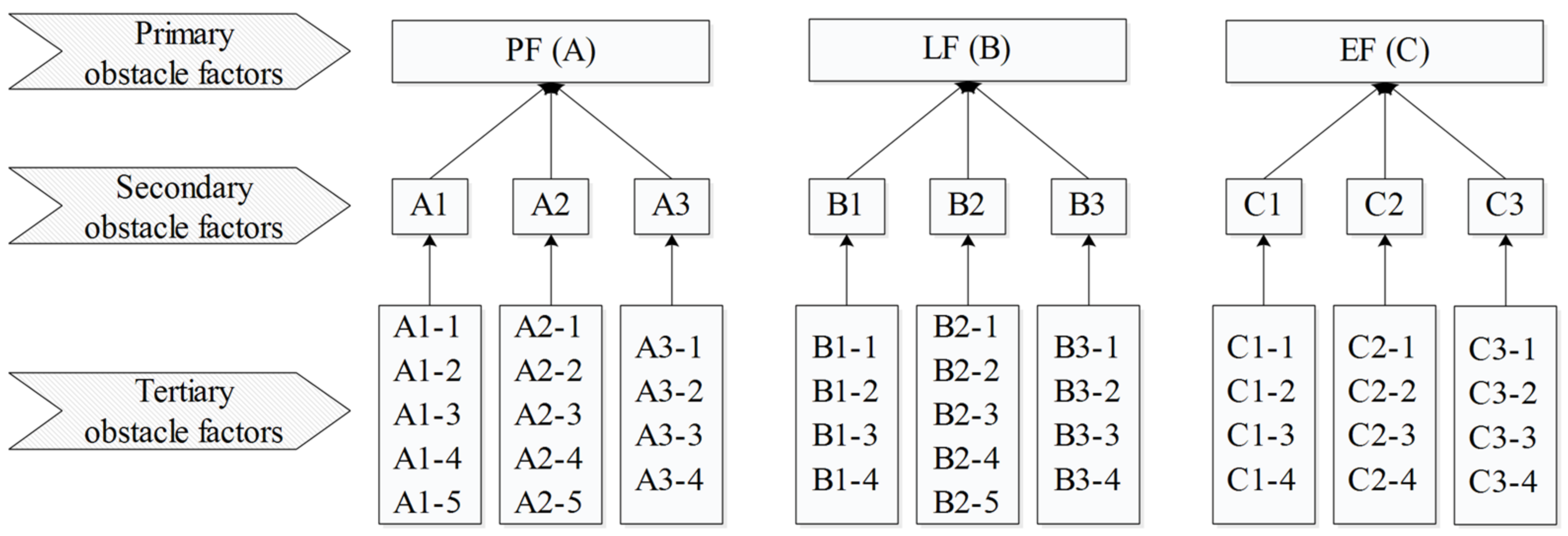
2.7. Obstacle Identification

After the statistical evaluation, it is crucial to conduct the identification of the obstacle factors that limit sustainable land use. This study constructed a three-level obstacle factors model (Figure 4).

Based on existing research [35,36], factor contribution ($F_j$), index deviation ($I_j$) and obstacle degree ($O_j$) were introduced to build the obstacle factor identification model.

Firstly, $F_j$ and $I_j$ were calculated:

$$F_j=u_j$$

(17)

$$I_j=1-X_j^{\prime }$$

(18)

Then, $O_j$ of each indicator was calculated:

$$O_j=\left(I_j\times F_j\right)/{{\displaystyle \sum }}_{j=1}^n{I}_j\times F_j$$

(19)

$O_j$ represents the obstacle degree of tertiary obstacle factors, then, obstacle degree of secondary and primary obstacle factors can be calculated.

$$Q_i={{\displaystyle \sum }}_{j=1}^n{O}_{ij}$$

(20)

where n refers to the indicator amount in the $i$th criterion.

3. Results

This study classified LUFs into 10 grades, which were level 1 (0–0.1), level 2 (0.1–0.2), level 3 (0.2–0.3), level 4 (0.3–0.4), level 5 (0.4–0.5), level 6 (0.5–0.6), level 7 (0.6–0.7), level 8 (0.7–0.8), level 9 (0.8–0.9) and level 10 (0.9–1.0). Similarly, D was classified by the same criterion. Based on the results, ESRI ArcGIS version 10.2© software and Origin 2017© were used to create the maps.

3.1. The Spatial and Temporal Characteristics of LUFs during 1996–2016

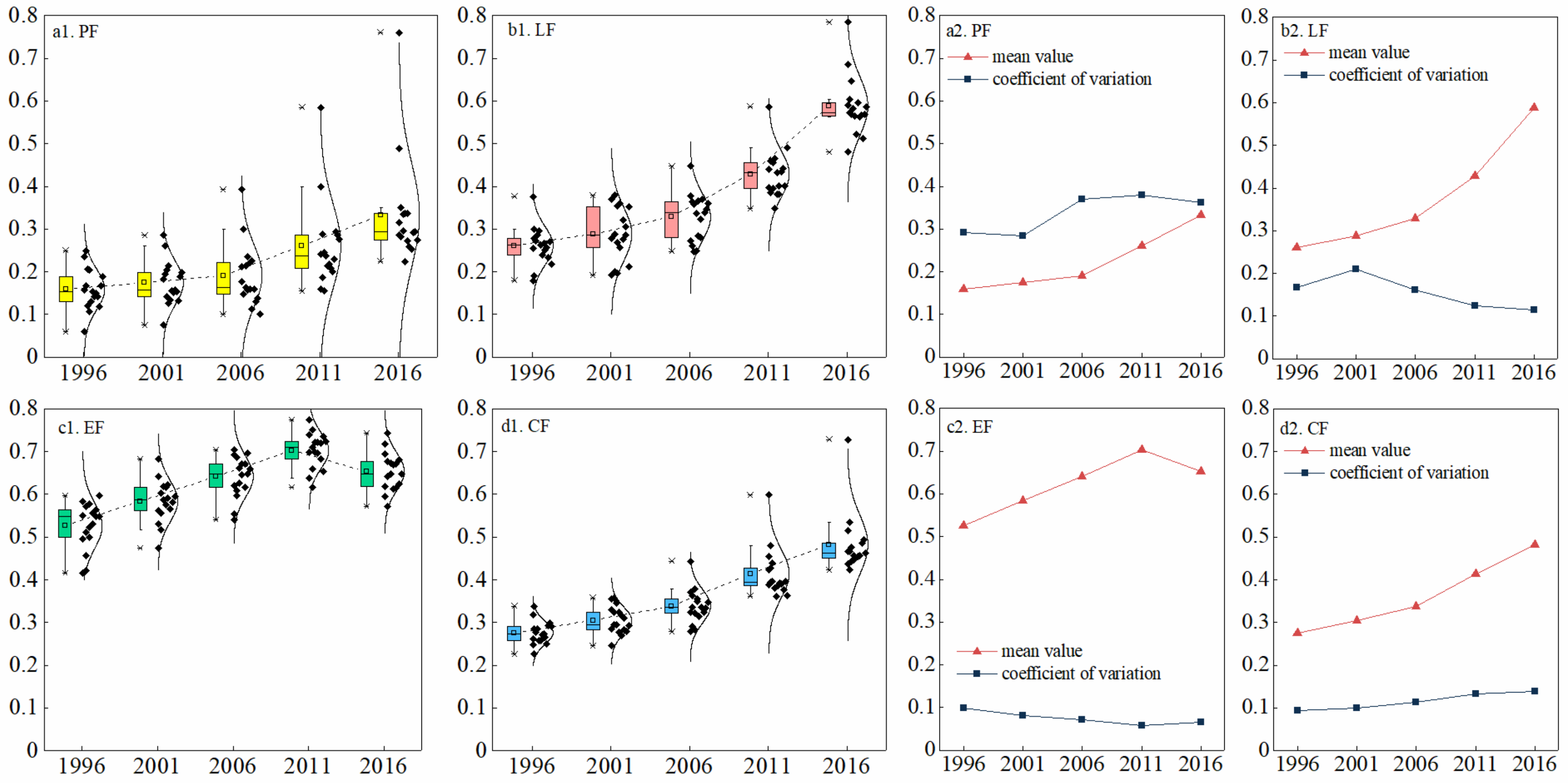
3.1.1. The Overall Level of LUFs during 1996–2016

It can be observed from Figure 5 that PF, LF, EF and comprehensive land use function (CF) has showed an overall upward trend during the study period, while the way of promotion varied with different dimensions. Specific analysis is as follows.

PF experienced a continuous enhancement during the study period. It increased slowly during 1996–2006, with a 20.16% enhancement in this decade. During 2006–2016, the increase speed of PF was significantly faster than that of the previous period, with an average incensement of 74.44%. $C_v$ decreased slightly, then significantly increased, and maintained a high level, showing that although PF was improved during the study period, the gap between regions had not narrowed, but showed greater differences. Compared with other dimensions, PF had the minimum mean value ($\sigma$) and the maximum coefficient of variation ($C_v$), indicating that PF was insufficient and unbalanced.

The trend of LF was similar to that of PF, but showed a faster rising tendency. LF raised slowly during 1996–2006, experienced a 25.92% increment, while it increased by 78.99% during 2006–2016. $C_v$ first increased then declined to a lower level continuously, indicating that the gap among 17 cities enlarged during 1996–2001 but continued to narrow during 2001–2016, and finally stabilized at a low level in 2016, reflecting a good balance among regions.

EF continued to increase during 1996–2011, but declined during 2011–2016. $C_v$ continued to decrease during 1996–2011, but increased a little during 2011–2016, which means, although EF was always with the maximum $\sigma$ and the minimum $C_v$ among all dimensions during the same period, it showed a trend of reduction and regional gap enlargement during 2011–2016. Therefore, attention needs to be paid to the utilization of ecological space.

CF is the result of the superposition of three dimensions. $\sigma$ continued to increase during 1996–2016, with the tendency similar to PF and LF. CF was still on the rise during 2011–2016. Benefit from the rapid rise of PF and LF, the impact of EF decline during the same period had been moderated. $C_v$ continued to increase at a slower rate during 1996–2016, and remained relatively smooth at a low level. From the previous analysis, it can be seen that the regional gap of PF was large, but after the weighting of LF and EF, regional gap narrowed, indicating that region with a high value of PF may had a low value of LF and EF.

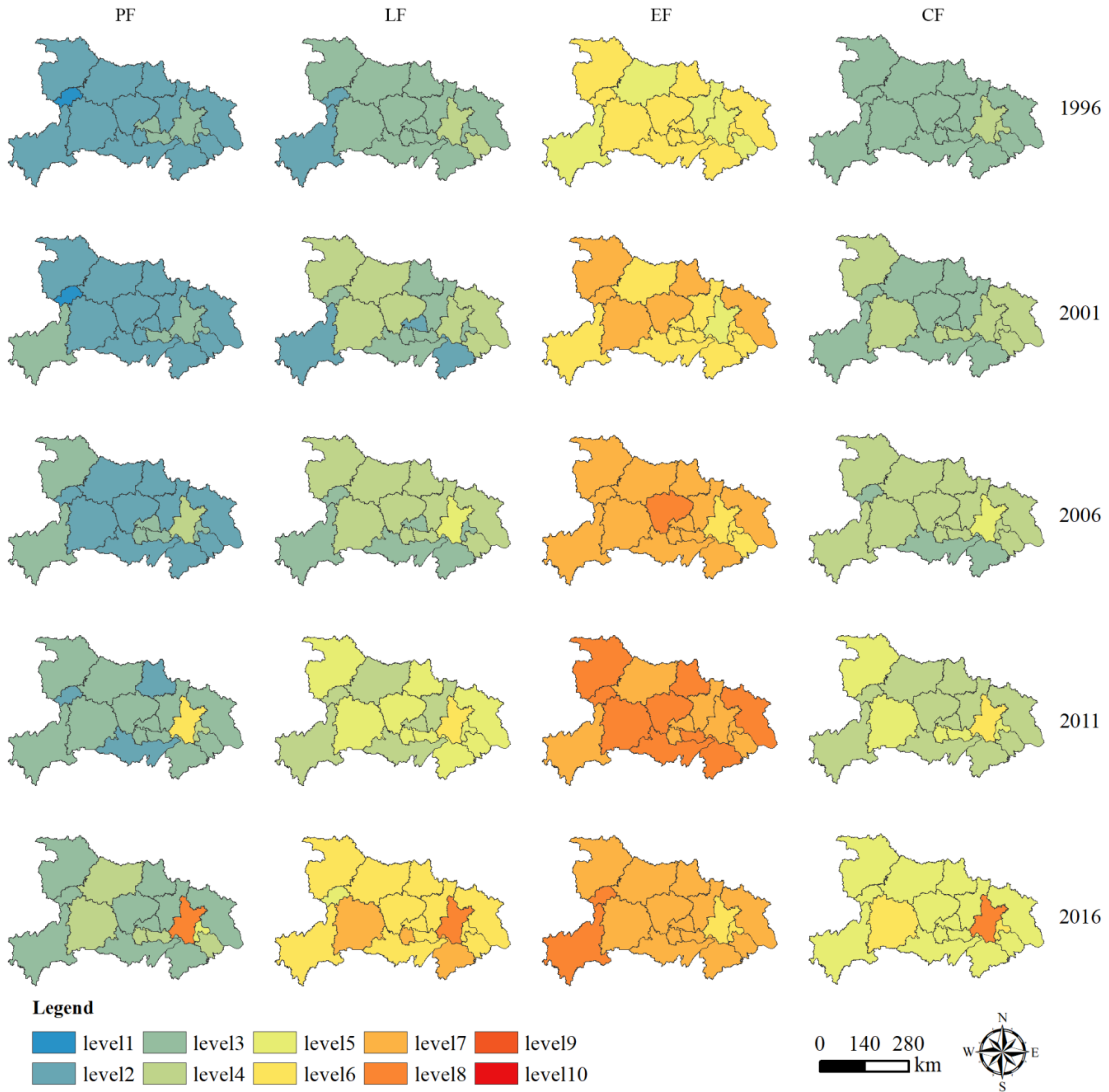
3.1.2. The Spatial Distribution of LUFs during 1996–2016

According to the above figure (Figure 6), PF was generally low, with 12 regions in the level2 zone in 1996. By 2001, the overall level of PF had increased slightly, but the increment was not sufficient to show up in the map. During 2001–2006, based on the build-up improvement in the previous stage, 5 cities were upgraded, no region was in level1 zone anymore. During 2006–2011, the overall level improved considerably with nine regions upgraded. During 2011–2016, 10 regions were upgraded and all regions were in level3 or a higher level zone. The highest quality regions and the lowest quality regions varied by two levels in 1996, four levels in 2011 and five levels in 2016, which also confirms that, although the overall level improved, the regional differences had increased.

Similar to PF, the overall level of LF was relatively low in 1996. By 2001, all regions were still located in level 2–4 zones, while the grade structure was optimized compared to 1996. During 2001–2006, eight regions were upgraded and no city was in the level2 zone anymore. During 2006–2011, 15 regions were upgraded by at least one level, of which, Ezhou and Xianning were upgraded by two levels. During 2011–2016, all regions were upgraded, while nine cities achieved a jump in level improvement. During the study period, all cities experienced at least two levels of improvement, showing a good state of development.

Compared to PF and LF, the overall level of EF was relatively high in 1996. By 2001, 10 cities were upgraded. Similarly, 10 regions had been upgraded by 2006. During 2006–2011, 11 regions were upgraded and all cities were in level7 and level8 zone. However, during 2011–2016, EF reversed its previous strong growth momentum and experienced an overall decline. In total, 10 regions were degraded and six regions remained the same, while Enshi was the only region upgraded in this period. In addition, with the overall decline of EF, there was a trend towards an expansion of regional differences. It should be noted that once a total decline occurs, enough attention should be paid to avoid the further deterioration of EF.

CF showed a relatively moderate state. In 1996, only Wuhan and Ezhou were located in level4 zone, the other 15 areas were all in level3 zone. By 2001, the grade structure was optimized compared to 1996. During 2001–2006, seven regions were upgraded and Wuhan was the only region in level5 zone. During 2006–2011, nine were regions upgraded and Wuhan was the only region in level6. During 2011–2016, CF experienced an overall promotion, with 14 cities upgraded. Wuhan was upgraded from level6 to level8, occupying an absolute leading position. Then Ezhou and Yichang were the only two regions in level6 zone, the remaining 14 areas were in level5 zone.

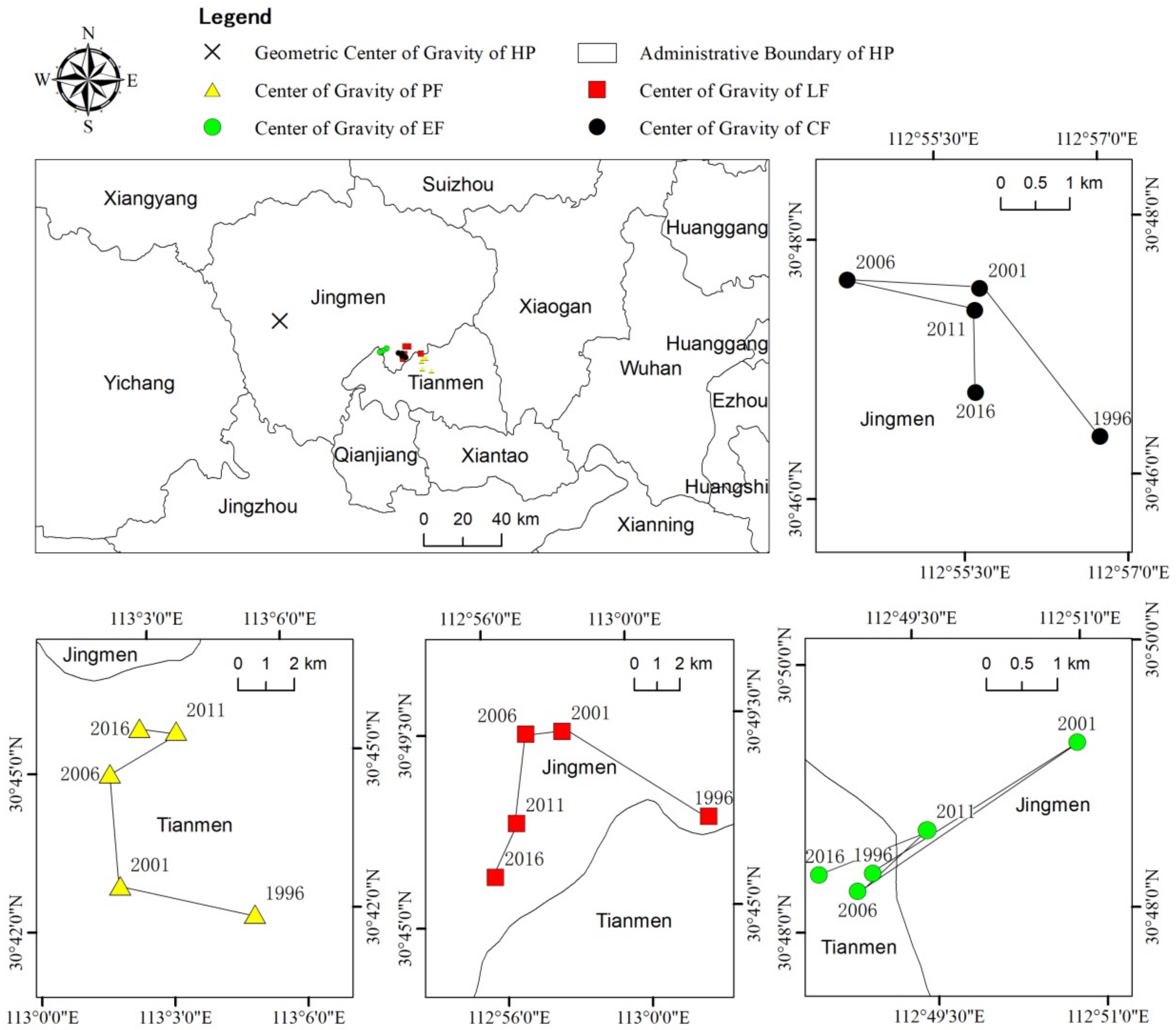
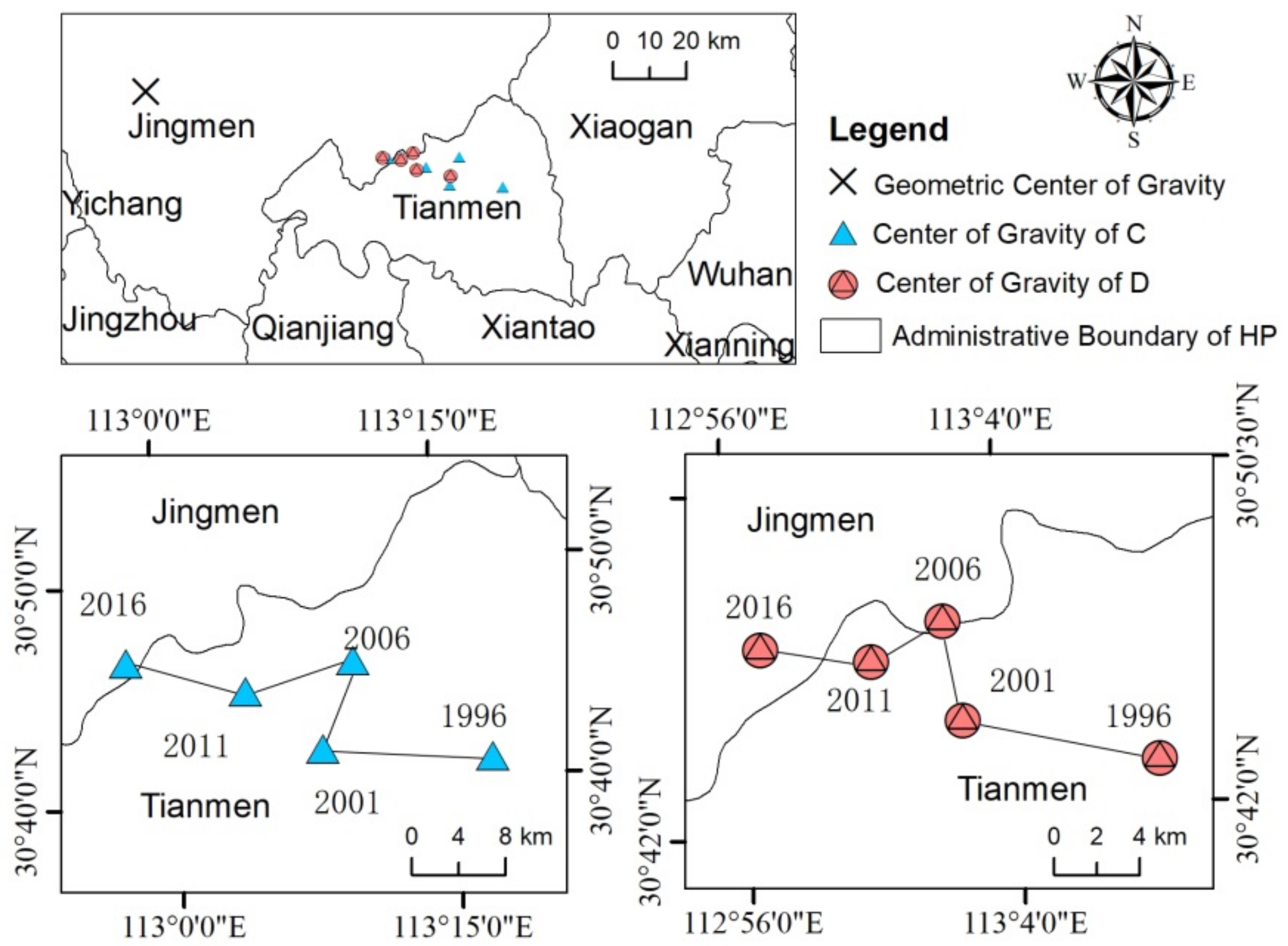
3.1.3. The Center of Gravity of LUFs during 1996–2016

Figure 7 shows that all the GCs were located in the southeastern part of HP’s geometric centers of gravity, which means that LUFs were higher in the east than in the west, and slightly higher in the south than in the north.

For PF, the movement pattern of GC can be described as “acceleration toward the north, deceleration toward the west” during 1996–2006, and “deceleration toward the north, east first, then west” during 2006–2016. Therefore, PF tends to be more spatially balanced in both north-south and east-west directions during 1996–2006. During 2006–2016, PF tends to be more balanced in the north-south direction while the spatial imbalance in the east-west direction has weakened.

For LF, the movement pattern of GC can be described as “deceleration to the west, north first and then south”. During 1996–2001, the displacement of GC toward the direction of geometric GC reached 7.41 km, indicating the spatial balance has improved considerably. Thereafter, GC shifted very little to the west during 2001–2016, and moved faster to the south in north-south direction, indicating that the balance in the east-west direction increased slightly and the imbalance in the north-south direction increased considerably.

For EF, the movement pattern of GC can be described as “northeast-southwest circulation”. After the back and forth “northeast-southwest” movement, GC shifted only 0.77 km in a straight line, with a direction of 89.03° south-west, showing that the spatial equilibrium of EF does not change much in north-south direction, and there is a small improvement in east-west direction.

For CF, the movement pattern of GC showed a uniform eastward trend and a deceleration northward trend during 1996–2006. In the following decade, GC showed the opposite movement of the previous decade. Overall, the spatial coordination of LUFs in HP was enhanced during the study period.

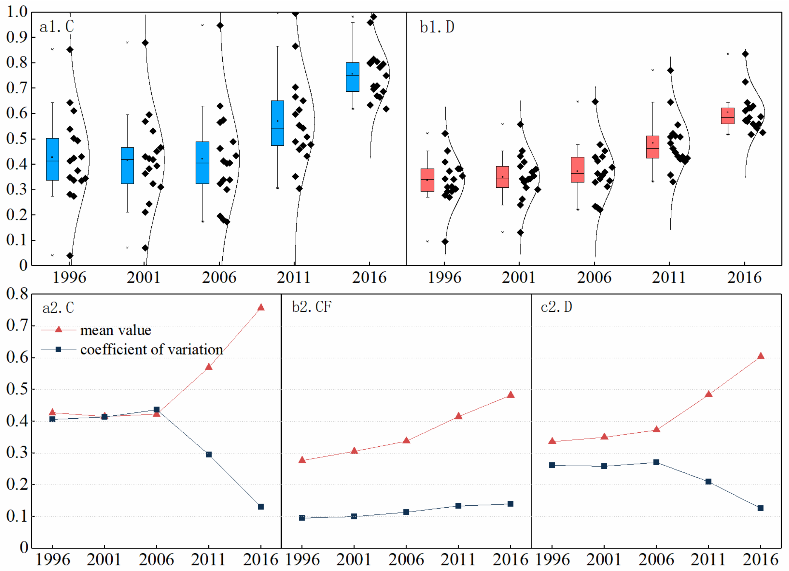
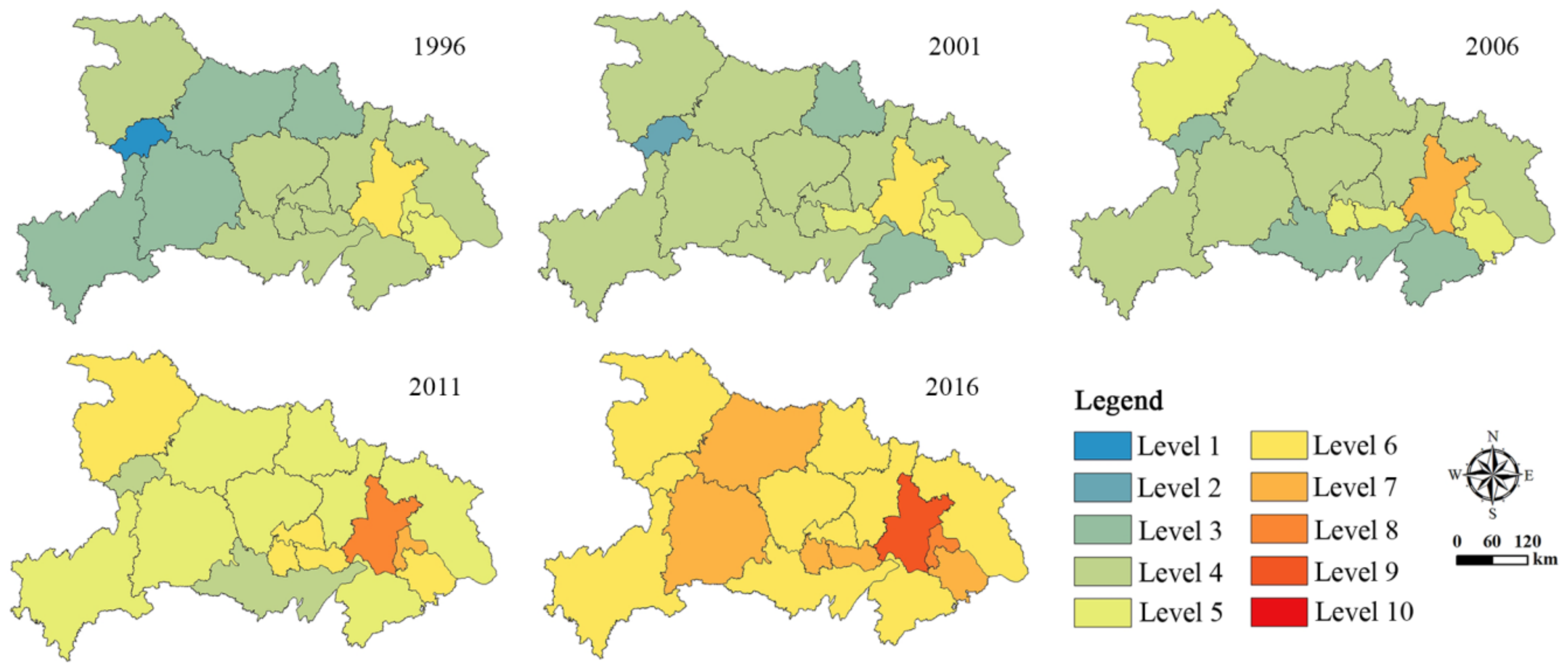
3.2. The Characteristics of Coupling Coordination Degree during 1996–2016

It can be seen from Figure 8 that during 1996–2006, the overall level of coupling coordination degree (D) in HP was low and regional difference was large, $\sigma$ increased by only 10.80% in 10 years, and $C_v$ maintained a high level. During 2006–2016, $\mathsf{\sigma }$ increased rapidly by 61.98%, and ${\mathrm{C}}_{\mathrm{v}}$ decreased by 53.56%, showing a good development momentum. It is worth noting, however, that the overall level of D in HP was only level4 in 1996–2006, level5 in 2011 and level6 in 2016. Although D experienced rapid growth during 2006–2016, the overall level is still not satisfactory and there is a lot of room for improvement.

In 1996, more than half of the regions were in level4 zone (Figure 9). Shennnongjia had the lowest coordination level due to the extremely unbalanced development of LUFs. EF of Shennongjia ranked first in HP with its unique ecological resource endowment, however, PF and LF of Shennongjia ranked lowest and second lowest respectively. During 1996–2001, the overall level of D improved, but the extend of improvement was not obvious. 5 regions were upgraded, and Xianning experienced a decline. During 2001–2006, the overall level of D experienced a small improvement, similar to the period 1996–2001. 5 regions upgraded and Jingzhou dropped by one grade. During 2006–2011, the overall level of D improved rapidly, benefiting from the narrowing gap of LUFs, and all the 17 cities were upgraded, of which, Ezhou, Xianning and Tianmen were raised by two levels. During 2011–2016, D still maintained the strong growth momentum of the previous period. Except Shiyan and Tianmen, the other 15 regions had achieved at least one level rise, of which Yichang, Xiangyang, Jingzhou and Shennong were upgraded by two levels. Wuhan was always the city with the highest coordination level during the study period and Shennongjia was the only city that saw its coordination level upgraded in all four phases of the study period.

From Figure 10, it can be seen that all the GCs were located in the east-southern part of HP’s geometric GC, indicating that C and D were higher in the eastern part than in the western part and slightly higher in the southern part than in the northern part. For D, the movement pattern of GC can be described as “continuous westward and fluctuating northward”, which means the spatial equilibrium in the east-west direction and north-south direction has been improved during the study period. During 1996–2006, GC decelerated to the west in the east-west direction and accelerated to the north in the north-south direction. The trajectory of the GC indicates that the spatial equilibrium of D in the east-west and north-south directions increased substantially during this period. During 2006–2016, GC continued to move westward in the east-west direction and southward first, then northward in the north-south direction. The trajectory of the GC indicates that the spatial equilibrium of D increased in the east-west direction and decreased slightly in the north-south direction during this period.

3.3. Diagnosis of Obstacle Degree of LUFs

3.3.1. Analysis of Obstacle Degree of Primary Obstacle Factors

For primary obstacle factors (

Table 2. Average degree of primary obstacle factors of HP (Unit: %).

Primary Obstacle Factors	1996	2001	2006	2011	2016
PF	55.25	56.88	58.08	59.83	60.65
LF	28.98	29.22	28.81	27.72	22.58
EF	15.77	14.54	13.12	12.45	16.77

), PF had the biggest barrier to CF and continued to increase during the study period. For LF, the obstacle degree increased during 1996–2001 and then decreased continuously. The overall obstacle degree showed a downward trend. For EF, the obstacle degree continued to decrease during 1996–2011, however, increased to a higher level rapidly during 2011–2016.

From the city level (Figure 11), for the obstacle degree of PF, only Wuhan and Ezhou decreased during the study period, while the other 15 cities increased to a greater or lesser degree. For the obstacle degree of LF, all the 17 regions decreased to a certain degree, of which, Yichang, Qianjiang, Tianmen, Jingzhou and Xianning declined significantly. For the obstacle degree of EF, eight regions increased, while the other nine regions declined slightly during the study period. It is worth noting that, during 1996–2011, only Wuhan and Ezhou increased slightly, while the other 15 regions declined to a greater or lesser degree. However, during 2011–2016, the obstacle degree of all regions had increased to varying degrees, indicating that the development trend had fluctuated considerably compared with the past.

3.3.2. Analysis of Obstacle Degree of Secondary Obstacle Factors

As for secondary obstacle factors (

Table 3. Average degree of secondary obstacle factors of HP (Unit: %).

Secondary Obstacle Factors	1996	2001	2006	2011	2016
A1 Input index	16.75	16.86	16.71	17.05	16.41
A2 Benefit index	26.23	26.88	27.22	27.97	28.64
A3 Intensity index	12.27	12.78	14.14	14.81	15.60
B1 Basic living index	7.37	6.69	6.41	7.05	5.35
B2 Comfort index	16.53	15.50	15.08	14.10	11.48
B3 Safety index	5.09	6.85	7.32	6.57	5.74
C1 Green index	8.14	8.01	7.88	8.36	9.64
C2 Threat index	3.65	3.00	2.83	2.30	1.89
C3 Governance index	3.97	3.43	2.41	1.79	5.24

), they had different variation characteristics. A2 continued to increase and always had the highest obstacle degree during the study period, indicating that A2 was the main short board that restricts sustainable land use. A1 fluctuated slightly during study the period and had the second highest obstacle degree in 2016. A3 continued to increase during the study period and ranked third in 2016. B2 ranked third in 1996, then continued to decline during 1996–2011 and ranked fourth in 2016. C1 declined during 1996–2006, and increased to a higher level during 2006–2016, ranked fifth in 2016. B1, B3, C2 and C3 had relatively low barriers and did not change much during the study period, of which B1 and C2 declined slightly while B3 and C3 increased slightly.

At the municipal level (Figure 12), secondary obstacle factors also showed different characteristics during the study period. (1) For A1, seven regions increased while the other 10 regions decreased. In 2016, Shennongjia and Shiyan had the lowest obstacle degree of 13.5%, while Ezhou had the highest obstacle degree of 20.0%. (2) For A2, except that Wuhan decreased significantly from 25.8% to 2.59%, all the other 16 regions increased their obstacle degree. (3) For A3, only Ezhou decreased during the study period, while the other 16 regions increased their obstacle degree. (4) For B1, only Wuhan increased its obstacle degree, while the other 16 regions decreased to varying degrees. (5) For B2, all the 17 regions decreased significantly, indicating an overall development of B2. (6) For B3, Shiyan, Yichang, Xianning and Qianjiang decreased their obstacle degree while other the 13 regions increased to a greater or lesser with different degree. (7) For C1, only Xianning and Xiaogan decreased, while the other 15 regions increased within the range from 8.4% to 19.1%. (8) For C2, only Ezhou increased, making it the region with the highest obstacle degree of 6.45% in 2016, while the other 16 regions decreased during the study period. (9) For C3, only Huangshi, Enshi and Shennongjia decreased their obstacle degree, while the other 14 regions increased within a different range. The increment of Wuhan, Yichang and Ezhou was among the top three, making them the regions with the highest obstacle degree in 2016.

(3) Analysis of obstacle degree of tertiary obstacle factorsWe have ranked the tertiary obstacle factors by obstacle degree and listed the top ten obstacle factors of each region, and the characteristics of the top 10 tertiary obstacle factors were analyzed (

Table 4. Characteristic of top 10 tertiary obstacle factors.

		1996	2001	2006	2011	2016
PF	Number	123	127	124	119	108
	Proportion (%)	72.35	74.71	72.94	70	63.53
	Total degree (%)	783.31	822	814.82	820.14	822.78
LF	Number	33	32	35	37	34
	Proportion (%)	19.41	18.82	20.59	21.76	20.00
	Total degree (%)	182.91	183.64	198.32	202.04	172.74
EF	Number	14	11	11	14	28
	Proportion (%)	8.24	6.47	6.47	8.24	16.47
	Total degree (%)	62.96	52.49	54.48	74.85	162.14
Top 10 obstacle factors	total	1029.18	1058.13	1067.62	1097.03	1157.66
	Proportion (%)	60.54	62.24	62.80	64.53	68.10

). (1) In 1996, the total degree of the top 10 obstacle factors in HP was 1029.18%, accounting for 60.54% of the total obstacle degree. Then the proportion continued to increase up to 68.10% by 2016, showing the characteristics of agglomeration, which means some of the main obstacle factors had more and more restriction on sustainable land use. (2) Obstacle factors that represent PF were always dominant during the study period. The proportion increased slightly then decreased to a lower level, while the obstacle degree increased, showing the characteristics of “the number decreased, the degree increased and ranked the top spot”. In 2016, except Wuhan, the top-ranked obstacle factors of all the other 16 region was A2-3. (3) Obstacle factors that represent LF changed a little during the study period, stable at around 20%, showing the characteristics of “the number and degree being stable and the ranking backward”. Obstacle factors with the highest frequency were B2-3 and B1-4. (4) Obstacle factors that represent EF remained at a low level during 1996–2011 while the quantity has been doubled during 2011–2016, showing the characteristics of “the number and degree increased and the ranking forward”. In 2016, obstacle factors ranked 2nd, 3rd and 7th in Wuhan represents EF.

4. Discussion

This study placed PF, LF and EF on an equally important level and established a three-dimensional indicator system including 39 indicators, which could evaluate land functions comprehensively. Besides, some indicators, like A2-3 Added-value of high and new technology industry per unit of land area, B3-2 Average rate of participation in basic pension insurance, basic medical care insurance and unemployment Insurance and C1-4 Wetland coverage rate were often not selected because their data would not be easily obtained and calculated [22,37,38]. Based on a long period of multi-channel collection, relevant data were obtained for this study, so these representative indicators were selected. This study demonstrated some innovation in the selection of indicators.

The early land use in China and other developing countries was at the expense of environment resources to some extent in exchange for rapid economic development [38,39]. According to the results, PF and LF showed a rapid growth trend during 2011–2016, while EF experienced an obvious decline, indicating that the improvement of PF and LF in HP was at the expense of EF to some extent. Further, cities of Wuhan and Ezhou experienced a rapid development of PF and LF during the study period, EF of the two cities, however, was degraded with a continuing downward trend during 2011–2016. This is because, with the population growth and rapid socio-economic development, the pressure exerted by the human society on resources and environment has gradually exceeded the capacity of natural environment after nearly two decades of accumulation, ultimately leading to a shrink of ecological space, an increase of ecological threats and incomplete ecological governance [40].

From a system theory perspective, it is a mode of operation that allows rapid development of one element at the expense of another, which may provide short-term benefits but is clearly unsustainable and will inevitably lead to the collapse of a system at some point if it remains unbalanced over time [41]. Therefore, land use should not be at the expense of one or another, but the performance of LUFs should be taken into account, thus realizing the coordinated and sustainable development of land use. From the above analysis, it can be seen that although the coupling coordination degree of LUFs in HP was steadily improved during 1996–2016, the absolute level of coordinated development was still relatively low, with 10 cities located in level6 coordinated zone, which means there is still a lot of room for improvement in the coordinated and sustainable development of land use in HP.

This paper diagnosed the obstacles that restrict sustainable land use from three levels. Results showed that PF was always dominant, and LF showed a downward trend, while EF showed an increasing trend. Benefit index (A2), Comfort index (B2) and Green index (C1) constituted the primary obstacle factors for each dimension. Added-value of high and new technology industry (A2-3) and land use intensity (A3-2) were key factors restricting PF. Number of medical practitioner (B1-4) and internet penetration rate (B2-3) were key factors restricting LF. Air quality rate (C3-1) and wetland coverage rate (C1-4) were key factors restricting EF. Therefore, PL utilization in HP should appropriately improve the intensity of land use and develop high-tech industries. LL utilization should focus on the improvement of medical care resources and developing internet industries. EL utilization should pay more attention to ecological land protection and ecological environment governance. Government departments should target and differentially regulate the development strategies of land use in different regions [42].

The study period began in 1996 and research data were mainly collected from the official statistical yearbook and government reports. Based on the availability and accuracy of data, this paper set research scale as municipal administrative division. In the future, with the standardization of statistics in statistical departments, researches can set research scale as county administrative division, which means more detailed researches on LUFs can be carried out. Moreover, this study designed an evaluation index system which contains a total of 39 indicators, which could evaluate the LUFs comprehensively. However, due to the actual land use situation of the study area, it is necessary to increase or decrease evaluation indexes, so as to make the evaluation results more scientific and practical.

5. Conclusions

This study firstly analyzed the connotation of LUFs based on the concept of sustainable development, and proposed an evaluation framework based on production-living-ecology function including 39 indicators. Entropy weight method was used to obtain LUFs of 17 cities in Hubei Province during 1996–2016, while regional center of gravity theory was used to describe the spatial-temporal variation characteristics of LUFs. Thirdly, the improved coupling coordination degree model was deduced to calculate the coupling coordination degree of the three aspects, embodied the idea of coordinated development of land space utilization. Finally, a three-level obstacle factors model was introduced to diagnose the obstacle degree of each indicator. The main conclusions can be drawn as follows:

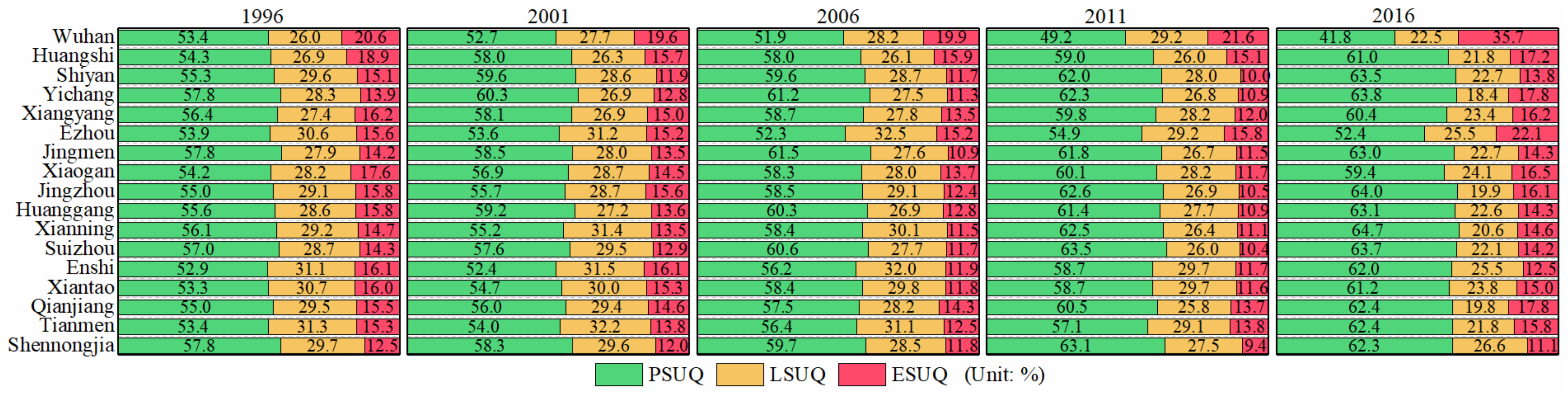
• PF, LF and CF continued to increase during the study period, and the increment during 2006–2016 was greater than 1996–2006 periods. EF increased steadily during 1996–2011, but suddenly declined during 2011–2016. The improvement of PF and LF in HP was at the expense of EF to some extent.
• The overall level of D increased slightly during 1996–2006 and significantly increased during 2006–2016. $C_v$ of D remained stable during 1996–2006, but declined rapidly during 2006–2016. The increase in the overall level and the decrease in the differences between regions reflect a good development trend. However, although D improved steadily, the absolute level in 2016 was still at a relatively low level, which means there was still a lot of room for improvement.
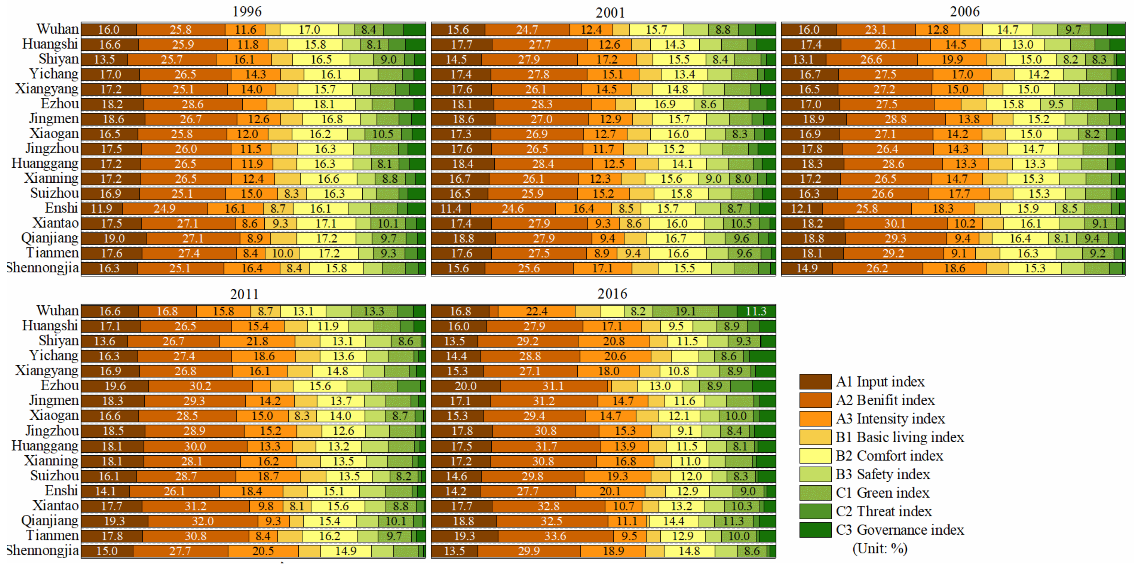
• For primary obstacle factors, PF was always dominant, LF showed a downward trend, EF decreased during 1996–2011 and increased to a higher level during 2011–2016. For secondary obstacle factors, Benefit index (A2), Comfort index (B2) and Green index (C1) constituted the primary obstacle factors of each dimension. In 2016, the obstacle degree from high to low was A2, A1, A3, B2, C1, B1, B3, C3 and C2. For tertiary obstacle factors, obstacle factors that represent PF showed the characteristics of “the number decreased, the degree increased and occupying the top spot”. LF showed the characteristics of “the number and degree being stable and the ranking backward”. EF showed the characteristics of “the number and degree increased and the ranking forward”. Further, some of the main obstacle factors had more and more restriction on sustainable land use. Added-value of high and new technology industry (A2-3) and land use intensity (A3-2) were key factors restricting PF. Number of medical practitioner (B1-4) and internet penetration rate (B2-3) were key factors restricting LF. Air quality rate (C3-1) and wetland coverage rate (C1-4) were key factors restricting EF.

Based on the above conclusions, this paper concluded with four recommendations for policy makers to advance the coordinated and sustainable development of land use.

5.1. Implement a Strict System of Land Use Regulation to Achieve Orderly Land Use

Firstly, a land use regulation system with clear hierarchy and classification management should be constructed. It is recommended that access conditions be set for different levels of areas, specifying the scale and intensity of development allowed in the area and the types of industries allowed, restricted and prohibited. A comprehensive use of administrative, economic and legal instruments could promote the implementation of the land use regulation system. Further, technical support and information platform construction should be strengthened to guarantee the scientific implementation. Finally, land use regulation cannot be achieved without strong regulation and enforcement.

5.2. Implement Industrial Layout Optimization Combined with Its Own Characteristics to Promote High-Quality and Sustainable Development of Land Use

Through reasonable industrial layout and industrial upgrading, the interconnection between metropolises, large, medium and small cities, and small towns is promoted, which is conducive to the radiation-driven effect of central cities on surrounding towns and rural areas, thus forming a new pattern of synergistic development between administrative divisions, as well as between urban and rural areas. In future land use processes, differentiated policies should be formulated according to the resource endowment and development orientation for each region, and the implementation of industrial layout of each region should be promoted by strengthening project support, deepening the mechanism between regions, and striving for sustainable and balanced development of land use.

5.3. Explore Underground Space Development to Open up a New Area of Land Use

Firstly, the comprehensive geological evaluation of underground space is a prerequisite for underground space use. Therefore, it is necessary to systematically carry out investigation and evaluation of underground space resources at the early stage of planning for future underground space use, and take the results of geological investigation and evaluation as the pre-requisite rigid constraints for underground space use planning. Further, the use of underground space is highly irreversible, so the planning of underground space should focus on the coordination with the planning of above-ground space. In addition, the management and operation of underground space should be strengthened, and the ecological and humanistic transformation of the underground space environment should be emphasized.

5.4. Unified Protection and Restoration of Mountains, Rivers, Forests, Fields, Lakes and Grasses to Solve Ecological Problems Should Be Adopted

First, it is suggested that the top-level design of resource and environmental economic policies be strengthened, giving it a more important role in ecological and environmental protection and sustainable development. Secondly, the authorities are advised to improve the emergency response mechanism for sudden ecological and environmental problems, making it scientific and operable. Thirdly, it is recommended that the market-oriented mechanism of ecological protection and restoration be explored, investment and financing channels be broadened, and a diversified investment mechanism be formed with government funds as the main body and social funds are widely absorbed.

References

1. Paracchini, M.L.; Pacini, C.; Jones, M.L.M.; Pérez-Soba, M. An aggregation framework to link indicators associated with multifunctional land use to the stakeholder evaluation of policy options. Ecol. Indic. 2011, 11, 71–80. [Google Scholar] [CrossRef]
2. Verstegen, J.A.; Karssenberg, D.; van der Hilst, F.; Faaij, A.P.C. Detecting systemic change in a land use system by Bayesian data assimilation. Environ. Model. Softw. 2016, 75, 424–438. [Google Scholar] [CrossRef] [Green Version]
3. Bach, P.M.; Staalesen, S.; McCarthy, D.T.; Deletic, A. Revisiting land use classification and spatial aggregation for modelling integrated urban water systems. Landsc. Urban Plan. 2015, 143, 43–55. [Google Scholar] [CrossRef]
4. Pérez-Soba, M.; Petit, S.; Jones, L.; Bertrand, N.; Briquel, V.; Omodei-Zorini, L.; Contini, C.; Helming, K.; Farrington, J.H.; Mossello, M.T.; et al. Land Use Functions—A Multifunctionality Approach to Assess the Impact of Land Use Changes on Land Use Sustainability; Springer: Berlin/Heidelberg, Germany, 2008; ISBN 9783540786474. [Google Scholar]
5. Liu, J.; Liu, Y.; Li, Y. Classification evaluation and spatial-temporal analysis of “production-living-ecological” spaces in China. ACTA Geogr. Sin. 2017, 72, 1290–1304. [Google Scholar]
6. Zhang, H.; Erqi, X.; Zhu, H. An ecological-living-industrial land classification system and its spatial distribution in China. Resour. Sci. 2015, 37, 1332–1338. [Google Scholar]
7. Jiaxing, C.; Jiang, G.; Jianwei, S.; Jing, L. The Spatial Pattern and Evolution Characteristics of the Production, Living and Ecological Space in Hubei Provence. China L. Sci. 2018, 32, 67–73. [Google Scholar]
8. Yang, J.; Li, Y.; Hay, I.; Huang, X. Decoding national new area development in China: Toward new land development and politics. Cities 2019, 87, 114–120. [Google Scholar] [CrossRef]
9. Nelson, E.; Mendoza, G.; Regetz, J.; Polasky, S.; Tallis, H.; Cameron, D.R.; Chan, K.M.A.; Daily, G.C.; Goldstein, J.; Kareiva, P.M.; et al. Modeling multiple ecosystem services, biodiversity conservation, commodity production, and tradeoffs at landscape scales. Front. Ecol. Environ. 2009, 7, 4–11. [Google Scholar] [CrossRef]
10. Jin, G.; Chen, K.; Wang, P.; Guo, B.; Dong, Y.; Yang, J. Trade-offs in land-use competition and sustainable land development in the North China Plain. Technol. Forecast. Soc. Chang. 2019, 141, 36–46. [Google Scholar] [CrossRef]
11. Peng, J.; Ma, J.; Du, Y.; Zhang, L.; Hu, X. Ecological suitability evaluation for mountainous area development based on conceptual model of landscape structure, function, and dynamics. Ecol. Indic. 2016, 61, 500–511. [Google Scholar] [CrossRef]
12. Knickel, K.; Renting, H.; van der Ploeg, J. Multifunctionality in European agriculture. In Sustaining Agriculture and the Rural Economy; Brouwer, F., Ed.; Edward Elgar Publishing Inc.: Cheltenham, UK, 2004; pp. 81–103. [Google Scholar]
13. Steinhäußer, R.; Siebert, R.; Steinführer, A.; Hellmich, M. National and regional land-use conflicts in Germany from the perspective of stakeholders. Land Use Policy 2015, 49, 183–194. [Google Scholar] [CrossRef]
14. Marshall, E.J.P.; Moonen, A.C. Field margins in northern Europe: Their functions and interactions with agriculture. Agric. Ecosyst. Environ. 2002, 89, 5–21. [Google Scholar] [CrossRef]
15. Gómez Sal, A.; González García, A. A comprehensive assessment of multifunctional agricultural land-use systems in Spain using a multi-dimensional evaluative model. Agric. Ecosyst. Environ. 2007, 120, 82–91. [Google Scholar] [CrossRef]
16. Wiggering, H.; Dalchow, C.; Glemnitz, M.; Helming, K.; Müller, K.; Schultz, A.; Stachow, U.; Zander, P. Indicators for multifunctional land use—Linking socio-economic requirements with landscape potentials. Ecol. Indic. 2006, 6, 238–249. [Google Scholar] [CrossRef]
17. Purushothaman, S.; Patil, S.; Francis, I.; König, H.J.; Reidsma, P.; Hegde, S. Participatory impact assessment of agricultural practices using the land use functions framework: Case study from India. Int. J. Biodivers. Sci. Ecosyst. Serv. Manag. 2013, 9, 2–12. [Google Scholar] [CrossRef]
18. Kates, R.W.; Clark, W.C.; Corell, R.; Hall, J.M.; Jaeger, C.C.; Lowe, I.; McCarthy, J.J.; Schellnhuber, H.J.; Bolin, B.; Dickson, N.M.; et al. Environment and development: Sustainability science. Science 2001, 292, 641–642. [Google Scholar] [CrossRef]
19. Zhou, D.; Xu, J.; Lin, Z. Conflict or coordination? Assessing land use multi-functionalization using production-living-ecology analysis. Sci. Total Environ. 2017, 577, 136–147. [Google Scholar] [CrossRef]
20. Nguyen, T.T.; Verdoodt, A.; Van Y, T.; Delbecque, N.; Tran, T.C.; Van Ranst, E. Design of a GIS and multi-criteria based land evaluation procedure for sustainable land-use planning at the regional level. Agric. Ecosyst. Environ. 2015, 200, 1–11. [Google Scholar] [CrossRef]
21. Zhen, L.; Cao, S.; Wei, Y.; Xie, G.; Li, F.; Yang, L. Land use functions: Conceptual framework and application for China. Resour. Sci. 2009, 31, 544–551. [Google Scholar]
22. Gaodi, X.; Lin, Z.; Caixia, Z.; Xiangzheng, D.; Koenig, H.J.; Tscherning, K.; Helming, K. Assessing the Multifunctionalities of Land Use in China. J. Resour. Ecol. 2010, 1, 311–318. [Google Scholar] [CrossRef]
23. Reidsma, P.; König, H.; Feng, S.; Bezlepkina, I.; Nesheim, I.; Bonin, M.; Sghaier, M.; Purushothaman, S.; Sieber, S.; van Ittersum, M.K.; et al. Methods and tools for integrated assessment of land use policies on sustainable development in developing countries. Land Use Policy 2011, 28, 604–617. [Google Scholar] [CrossRef]
24. Liu, C.; Xu, Y.; Sun, P.; Liu, J. Progress and prospects of multi-functionality of land use research. Prog. Geogr. 2016, 35, 1087–1099. [Google Scholar]
25. Hou, X.; Liu, J.; Zhang, D. Regional sustainable development: The relationship between natural capital utilization and economic development. Sustain. Dev. 2019, 27, 183–195. [Google Scholar] [CrossRef] [Green Version]
26. Fang, F.; Qiao, L.L.; Ni, B.J.; Cao, J.S.; Yu, H.Q. Quantitative evaluation on the characteristics of activated sludge granules and flocs using a fuzzy entropy-based approach. Sci. Rep. 2017, 7. [Google Scholar] [CrossRef] [PubMed] [Green Version]
27. Zhang, Z.; Zhou, M.; Ou, G.; Tan, S.; Song, Y.; Zhang, L.; Nie, X. Land suitability evaluation and an interval stochastic fuzzy programming-based optimization model for land-use planning and environmental policy analysis. Int. J. Environ. Res. Public Health 2019, 16, 4124. [Google Scholar] [CrossRef] [Green Version]
28. Liu, D.J.; Li, L. Application study of comprehensive forecasting model based on entropy weighting method on trend of PM2.5 concentration in Guangzhou, China. Int. J. Environ. Res. Public Health 2015, 12, 7085–7099. [Google Scholar] [CrossRef] [PubMed] [Green Version]
29. Wang, R.; Cheng, J.; Zhu, Y.; Lu, P. Evaluation on the coupling coordination of resources and environment carrying capacity in Chinese mining economic zones. Resour. Policy 2017, 53, 20–25. [Google Scholar] [CrossRef]
30. Cheng, X.; Long, R.; Chen, H.; Li, Q. Coupling coordination degree and spatial dynamic evolution of a regional green competitiveness system—A case study from China. Ecol. Indic. 2019, 104, 489–500. [Google Scholar] [CrossRef]
31. Li, Y.; Wang, J.; Liu, Y.; Long, H. Spatial pattern and influencing factors of the coordination development of industrialization, informatization, urbanization and agricultural modernization in China: A prefecture level exploratory spatial data analysis. Acta Geogr. Sin. 2014, 69, 199–212. [Google Scholar] [CrossRef]
32. Walker, F.A. Restriction of immigration. JAMA J. Am. Med. Assoc. 1891, XVII, 938. [Google Scholar] [CrossRef] [Green Version]
33. Aboufadel, E.; Austin, D. A new method for computing the mean center of population of the United States. Prof. Geogr. 2006, 58, 65–69. [Google Scholar] [CrossRef]
34. Chen, Y.; Luo, J. Derivation of relations between urbanization level and velocity from logistic growth model. Geogr. Res. 2002, 25, 1063–1072. [Google Scholar] [CrossRef]
35. Chen, Y.; Luo, J. Dynamic Evaluation of Land Use Functions Based on Grey Relation Projection Method and Diagnosis of Its Obstacle Indicators: A Case Study of Guangzhou City. Geogr. Res. 2006, 25, 1063–1072. [Google Scholar] [CrossRef]
36. Wei, C.; Wang, Z.; Lan, X.; Zhang, H.; Fan, M. The spatial-temporal characteristics and dilemmas of sustainable urbanization in China: A new perspective based on the concept of five-in-one. Sustainability 2018, 10, 4733. [Google Scholar] [CrossRef] [Green Version]
37. Liu, C.; Xu, Y.; Huang, A.; Liu, Y.; Wang, H.; Lu, L.; Sun, P.; Zheng, W. Spatial identification of land use multifunctionality at grid scale in farming-pastoral area: A case study of Zhangjiakou City, China. Habitat Int. 2018, 76, 48–61. [Google Scholar] [CrossRef]
38. Wang, L.; Li, F.; Gong, Y.; Jiang, P.; Huang, Q.; Hong, W.; Chen, D. A quality assessment of national territory use at the city level: A planning review perspective. Sustainability 2016, 8, 145. [Google Scholar] [CrossRef] [Green Version]
39. Xie, H. Towards Sustainable Land Use in China: A Collection of Empirical Studies. Sustainability 2017, 9, 2129. [Google Scholar] [CrossRef] [Green Version]
40. Wei, Y.D.; Ye, X. Urbanization, urban land expansion and environmental change in China. Stoch. Environ. Res. Risk Assess. 2014, 28, 757–765. [Google Scholar] [CrossRef]
41. Pretty, J.; Benton, T.G.; Bharucha, Z.P.; Dicks, L.V.; Flora, C.B.; Godfray, H.C.J.; Goulson, D.; Hartley, S.; Lampkin, N.; Morris, C.; et al. Global assessment of agricultural system redesign for sustainable intensification. Nat. Sustain. 2018, 1, 441–446. [Google Scholar] [CrossRef]
42. He, C.; Han, Q.; de Vries, B.; Wang, X.; Guochao, Z. Evaluation of sustainable land management in urban area: A case study of Shanghai, China. Ecol. Indic. 2017, 80, 106–113. [Google Scholar] [CrossRef]
Figure 1. Production–living–ecological land and production–living–ecological functions. (Source: made by authors).
Sustainability 13 00996 g001
Figure 2. Functional superposition and multi-functions of land use. (Source: made by authors).
Sustainability 13 00996 g002
Figure 3. Location map of study area (source: made by authors).
Sustainability 13 00996 g003
Figure 4. Three-level obstacle factors of LUFs (Source: made by authors).
Sustainability 13 00996 g004
Figure 5. The characteristics of land use functions (LUFs) of Hubei Province (HP) during 1996–2016. (Source: made by authors).
Sustainability 13 00996 g005
Figure 6. The spatial distribution of LUFs during 1996–2016.
Sustainability 13 00996 g006
Figure 7. The migration of center of gravity (GC) of LUFs during 1996–2016 (source: made by authors).
Sustainability 13 00996 g007
Figure 8. The characteristics of coupling coordination degree during 1996–2016 (source: made by authors).
Sustainability 13 00996 g008
Figure 9. The spatial distribution of coupling coordination degree during 1996–2016.
Sustainability 13 00996 g009
Figure 10. The migration of GC of C and D during 1996–2016 (source: made by authors).
Sustainability 13 00996 g010
Figure 11. The ratio of primary obstacle factors during 1996–2016 (source: made by authors).
Sustainability 13 00996 g011
Figure 12. The ratio of secondary obstacle factors during 1996–2016.
Sustainability 13 00996 g012