Abstract
Earthquakes are one of the most overwhelming types of natural hazards. As a result, successfully handling the situation they create is crucial. Due to earthquakes, many lives can be lost, alongside devastating impacts to the economy. The ability to forecast earthquakes is one of the biggest issues in geoscience. Machine learning technology can play a vital role in the field of geoscience for forecasting earthquakes. We aim to develop a method for forecasting the magnitude range of earthquakes using machine learning classifier algorithms. Three different ranges have been categorized: fatal earthquake; moderate earthquake; and mild earthquake. In order to distinguish between these classifications, seven different machine learning classifier algorithms have been used for building the model. To train the model, six different datasets of India and regions nearby to India have been used. The Bayes Net, Random Tree, Simple Logistic, Random Forest, Logistic Model Tree (LMT), ZeroR and Logistic Regression algorithms have been applied to each dataset. All of the models have been developed using the Weka tool and the results have been noted. It was observed that Simple Logistic and LMT classifiers performed well in each case.
1. Introduction
In the early ages, earthquakes were believed to have occurred due to certain supernatural forces [1,2]. It was none other than Aristotle (384–322 B.C.) who first described earthquakes as natural phenomena and outlined some of the possible causes behind them in a truly scientific way. Earthquakes represent one of the most devastating natural hazards. Strong earthquakes are often disastrous. Countries including Japan, the USA, countries and China as well as countries in the middle and far east experience destructive earthquakes from time to time [3]. India has also experienced a number of large and medium sized earthquakes that have caused an enormous loss of lives and damage to properties [4,5]. The earthquake that struck Maharastra in the early morning of 30th September 1993 was one of the most devastating earthquakes ever recorded. Effective forecasting methods for the occurrence of the next strong earthquake event may enable us to mitigate loss of life and damage to property; this is one of the prime objectives for researchers in earthquake seismology [6,7].
Approximately 90% of all earthquakes are natural, resulting from the occurrence of tectonic events [8,9]. The remaining 10% are related to volcanism, man-made effects or other factors. Natural earthquakes are usually much stronger than other types of earthquakes and are caused by internal changes within the Earth. Two theories are related to earthquakes: the first one is the continental drift theory and the second one is the plate-tectonic theory.
Any shaking of the ground may be termed as an earthquake. There are two types of earthquake: natural earthquakes and man-made earthquakes, otherwise known as artificial earthquakes or induced seismicity (seismic events that are a result of human activity). In the case of man-made earthquakes, there are many different ways in which human activity can cause induced seismicity, including geothermal operations, reservoir impoundment (water behind dams), wastewater injections as well as oil and gas operations such as hydraulic fracturing. Some man-made explosions including chemical or nuclear explosions can cause vibrations on the free surface. Typically, minor earthquakes (of very low magnitude) and tremors alter the stresses and strains on the Earth’s crust.
The continental drift theory describes how continents change position on the Earth’s surface. Abraham Ortelius, a Dutch geographer first introduced the idea of continental drift in 1596. Then, in 1620 Francis Becon provided a similar opinion on the basis of geometrical similarity between the coast lines of Brazil and Africa. This theory was modified by many researchers. The hypothesis that continents “drift” was fully developed by Alfred Wegner in 1912. He suggests that the continents were once squeezed into a single proto continent which he called Pangaea. He suggested that over time these continents have floated apart into their current distribution. Although Wegner presented a great deal of documentation for continental drift, he was unable to produce a conclusive clarification for the physical procedure which might have caused this drift. After the conception of the theory of palaeomagnetism, Wegner’s theory began to be dismissed and a considerable basis for the theory of plate tectonics was discussed by [10,11].
The plate-tectonic theory, a significant scientific advancement of the 1940s, is based on two major scientific concepts involving sea-floor spreading [12,13]. The interior structure of the Earth is radially layered. These layers include the crust, upper mantle, lower mantle, outer core and inner core, as discussed by [14].
Investigations of the mechanisms behind earthquakes were initiated by the works of Reid [15,16], who formulated the theory of elastic rebound based on the study of the 1906 California earthquake. In the 1970s scientists tried to determine an accurate method to predict earthquakes, but no significant achievements were made.
A popular branch of seismology involves earthquake forecasting, which assesses the frequency and magnitude of earthquakes in a particular area over years, or decades, determining the general level of earthquake seismic hazard probabilistically (see refs. [17] and [18]). The goal of earthquake forecasting is the correct assessment of three elementary factors, namely, the time, place and size of the predicted earthquake—often differentiated from earthquake prediction. The problem of earthquake prediction is extremely difficult and involves a number of socio-economic problems. A prediction is useful only when it is accurate in both time and place. Although the prediction program has not yet been perfected in nature. There is significant progress in this direction during the last 50 years. Certain precursory items have been identified. Those items may have a strong relationship with the occurrence of an impending earthquake. Such precursory data has been reviewed by [19]. Some of the most recent data may be summarized as:
- Anomalous animal behavior: the anomalous behavior of animals such as cattle, dogs, cats, rats, mice, birds, fish, snakes and so on before a large earthquake has been considered in [20,21]. Abnormal behavior and more intensive responses of animals are observed during the high magnitude of the earthquake (5 or more). These responses are mostly observed in the epicentral region—close to the active faults. It has been reported that they are actually re-responding to the P-wave, which was first outlined by [18,22]. It was also discussed that the precursor time may vary from a few minutes to various hours or even for several days, with increased restlessness before an earthquake.
- Hydrochemical Precursors: During the seismically inactive period, it has been observed that absorption levels of deliquescing minerals and gassy integrands of underground water in a seismically active region remain almost constant [23,24].
- Temperature Change: It has been reported that in Lunglin in China (1976) and Przhevalsk in Russia (1970), a tolerable rise of temperature by 10 °C and 15 °C occurs before earthquakes [25,26].
- The changes in water level in the wells and radon control were quoted by many seismologists from the U.S., Japan and China as precursory data [27,28].
- The frequency of minor shocks increases, at first gradually. Then it is drastically followed by a pause in the earthquake activity. This has been termed as the seismic time gap. The seismic time gap has been interpreted as an indication of an impending earthquake. Notably, a large earthquake near the city of Haicheng in Liaonping province in China in February 1975 was successfully predicted using a seismic time gap indication. This issue was extensively discussed in [29], and also by many researchers.
- On the basis of the study of foreshocks, a few earthquakes have been effectively predicted. In general, extensive earthquakes are preceded by slight shocks, which are known as foreshocks. In November 1978 foreshock observations were successfully used to predict an earthquake in Mexico. In India, the Bhuj earthquake in January 2001 was also preceded by foreshocks in December 2000. In 2006, the results presented in [30] indicated that earlier predictions were inaccurate. In particular, there was no formal short-term prediction, even though the alike prediction was prepared by individual scientists.
- Changes in the P-wave velocity (Vp), S-wave velocity (Vs) as well as their ratio Vp/Vs may be considered as important precursory items to an impending earthquake. The prediction of occurrence time could almost be deterministic in a favorable case, as claimed by [31]. A Vp/Vs anomaly failed to occur, which was based on 1976 prediction of a M 5.5 to M 6.5 earthquake close to Los Angeles [32].
This paper mainly aims to predict earthquakes in India in general and the upper part of India specifically before they occur. To realize this, an analysis of seven classifiers was conducted. The investigation was realized using the Weka tool. The investigation was realized for six different earthquake datasets. Then, a comparison was conducted. The novelty of this research is that almost a 98% chance of predicting the right magnitude range of earthquakes has been achieved. This has significant social impacts.
2. Methods
In this research, 6 different datasets of the earthquake were used. The source of data is database indicated in [33]. According to the new study of Earthquake Disaster Risk Index factor of India [34], 50 Indian cities face the risk of earthquakes. This study considered 13 out of the 50 cities that have a high risk of earthquakes. It also included 15 cities that have a medium risk. A total of 28 of these cities are in North India, Gujarat, the North East of India, Uttar Pradesh, Bihar and the Andaman & Nikobar islands. As a result, all past earthquake information for a particular state that contains these high-risk cities was collected in a single dataset. Hence, five different datasets viz., Andaman & Nikobar, Gujarat, North India, North East India, UP Bihar and Nepal were considered. Since most of the cities in these dataset are in Northern India, one dataset was prepared including Northern India and the nearby country Nepal. For classification, the Weka tool was used in this research. Weka is a powerful tool for Data Mining, pre-processing, classification, clustering, visualization and regression [35]. This tool uses java programming. The Weka tool was used to train the machine learning model and test its performance. The results of the machine learning model can be obtained in the forms of Precision, Recall, Accuracy, F-Measure, MCC, confusion matrix, etc. The earthquake dataset from 1900 to 2020 for different states of India and the nearby country of Nepal was used. The description of the datasets has been discussed in Table 1. The total number of instances mentioned in Table 1 is the total number of earthquakes.

Table 1.
Database set and the descriptions for the algorithms.
The distribution of the class variable is shown in Figure 1.
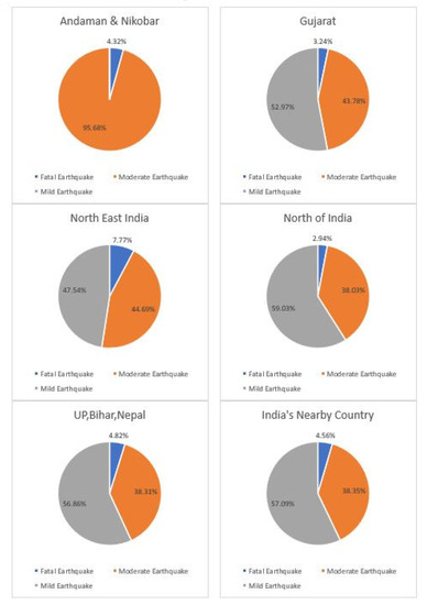
Figure 1.
The class variable distribution in each dataset.
The geographical map in Figure 2 presents the area that was used to build the machine learning model. Also, Figure shows the dataset information on a map.
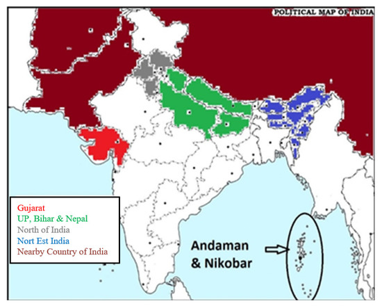
Figure 2.
Dataset Region.
Each dataset has 20 attributes and 1 target variable. The target variable has 3 class viz., Mild Earthquake, Moderate Earthquake and Fatal Earthquake. The target variable contains three class. It was divided using magnitude values:
- For Fatal Earthquakes, magnitude values greater than 5.5 were used.
- For Moderate Earthquakes, magnitude values of between 4.5 and 5.5 were used.
- For Mild Earthquakes, magnitude value less than 4.5 values were used.
The descriptions of dataset attributes have been provided in Table 2. The dataset has been divided into 2 parts: training and testing. Both parts have been divided into equal sections for all of the datasets [36]. The model was trained using the training dataset and the accuracy of the testing dataset was noted. Each model is capable of predicting the categories of earthquakes i.e., Fatal Earthquake, Moderate Earthquake and Mild earthquake. As a result, the magnitude range could be identified.
Table 2.
Database attributes description.
To train the model, the following classification machine learning algorithm was used in the Weka tool.
2.1. Bayes Net
The Bayesian network comes under the category of a probabilistic graphical model and therefore contains nodes and directed edges. Both relationship conditionally dependent and conditionally independent variables have been utilized in this model. The model was trained based on the probability of events. To design the Bayes Network, three elements were required: Random Variables; a Conditional Relationship; and Probability Distributions. It is a type of eager algorithm but this means it requires more computational time. The Bayesian network algorithm can be used in many fields like artificial intelligence, the medical field, the environmental field, etc. [37].
2.2. Random Forest
Random forest is a type of supervised machine algorithm. It creates a random decision tree and merges it into a single forest. To improve accuracy, it includes a decision model. It is also a type of ensemble learning method used for classification. The main difference between the decision tree and the random forest is that the random forest generates a root node feature by randomly splitting. The Random forest selects a random feature for improving the performance of its accuracy. As compared to the bagging and boosting method, the random forest method is faster [38]. In some cases, the random forest provides better results when using the Support Vector Machine, which is a neural network.
2.3. Simple Logistic Regression
Simple logistic regression is very similar to linear regression, except for the fact that in simple logistic regression the dependent attribute should be nominal, rather than being a measurement. In Simple logistic regression, one goal is for the probability of a specific value of the nominal attribute to be associated with the measurement attribute. Another goal is to predict the probability of particular attributes based on the measurement attribute. Simple logistic regression is similar to linear regression, but it works based on the nominal target variable [39]. It finds the equation that provides the best fit to predict the value of the target variable for every value of the input variable.
2.4. Random Tree
A Random tree is a type of classification algorithm that is designed by using a stochastic process. It is a type of ensemble learning algorithm that produces a lot of discrete learners [40]. It also works like a decision tree. In the decision tree on every split, the subset is not random; however, in a random tree, only a random subset of attributes is available on each split of the node. Each node of the tree represents an input attribute. The number of edges of the tree is equal to the possible number of input attributes. The random tree works on both classification and regression type problems.
2.5. Logistic Model Tree (LMT)
A Logistic Model Tree (LMT) is a type of supervised machine learning algorithm. It is a combination of logistic regression and a decision tree. This algorithm works based on former knowledge of a model tree. It is a type of decision tree where the leaves use linear regression models to provide a piecewise form of linear regression. Every node of a tree is produced using the Linear Regression (LR) model by the LogitBoost algorithm. LMT uses cross-validation for finding the number of Logiboost iterations [41]. The additive least-square logistic regression is used by the Logiboost algorithm for each class. In the LMT model, the linear logistic regression model is used for computing the subsequent probability of leaf nodes.
2.6. ZeroR
ZeroR is the simplest classification algorithm. ZeroR depends on the relevant target and disregards all other relevant predictors. It also predicts the majority class, though there is no predictability power in the ZeroR algorithm. It creates a frequency table of the target variable and selects the most frequent value. The algorithm is beneficial for determining a baseline performance as a standard for other classification algorithms. The ZeroR classifiers work using frequency as the main classification method. The ZeroR classifiers take a class variable and construct the frequency table of the class variable. The ZeroR algorithm does not use any rule, as a result, it is known as the ZeroR classifier [42].
2.7. Logistic Regression
Logistic regression is a type of classification algorithm that is used when the target variable belongs to a certain type of category. It is a predictive algorithm and works based on the concept of a probability model. It is a type of linear regression but it uses the complex cost function i.e., the sigmoid function. The logistic regression hypothesis tends to occur in between 0 and 1. It represents an equation that is very similar to linear regression. That is why this algorithm involves regression. The logistic regression works using a logistic function. It estimates the parameters of a logistic model [43].
To evaluate these machine learning classifier algorithms, the results of the following factors have been noted:
- Accuracy: Machine learning classifier accuracy is the technique used to measure the performance of the classifier. The accuracy result is noted in the corrected prediction percentage of the data.
- Precision: Precision is the fraction of the corrected positive predicted value to the total positive predicted value. It is also known as Specificity.
- Recall: Recall is the fraction of the corrected positive predicted value to the positive predicted value. It is also known as Sensitivity.
- F- Measure: F-Measure is calculated from the precision and the recall. It is the harmonic mean of precision and recall. It is used the measure the accuracy of the test.
- Matthews Correlation Coefficient (MCC): MCC is the measure used to check the quality of classification. It is also known as the phi coefficient.
- Kappa Statistics: The Kappa Statistic is the most commonly used statistic for test interrater consistency. A kappa of 1 indicates perfect agreement, while a kappa of 0 indicates a chance level.
3. Result and Performance
This section includes the results of different datasets. Each dataset result has been described in the table format of the various classification algorithms. For each classification algorithm along with accuracy, the Precision, Recall, F-Measure, MCC, and Kappa Statistics were also calculated.
3.1. Results for Andaman & Nikobar
For the Andaman & Nikobar dataset, the Simple Logistic and LMT methods achieved the highest accuracy rate of 99.94%. The Precision and Recall rates of the Simple Logistic and LMT methods were 99.9%. The Bayes Net method was the next best performing method after the Simple logistic and LMT methods. The Bayes Net method achieved a 99.82% accuracy rate, and 99.8% Precision and Recall rates. The Random Forest method achieved a 97.37% accuracy rate, a 97.50% Precision rate and a 97.40% Recall rate. The Random Tree method achieved a 99.04% accuracy rate, a 99.90% Precision rate and a 99.90% Recall rate. The Logistic Regression achieved a 98.68% accuracy rate, a 98.70% Precision rate and a 98.70% Recall rate. For the Andaman & Nikobar dataset, ZeroR provided the worst accuracy rate. The ZeroR method achieved a 61.01% accuracy rate, a 61.8% Precision rate and a 61.00% Recall rate. Table 3 shows the Andaman & Nikobar dataset results for various classification algorithms.
Table 3.
Comparison of different classification algorithms for Andaman & Nikobar.
3.2. Results for Gujarat
For the Gujarat dataset, the Bayes Net, Simple Logistic and Random Tree methods achieved the highest accuracy rate of 98.18%. The Precision and Recall rates for the Bayes Net, Simple Logistic and Random Tree methods were 98.3% and 98.20%, respectively. After the Bayes Net method, the next best performing methods were the Simple Logistic, Random Tree, Random Forest and LMT methods. The Random Forest method achieved a 96.36% accuracy rate, a 96.40% Precision rate, and a 95.40% Recall rate. The LMT achieved a 96.36% accuracy rate, a 96.30% Precision rate, and a 96.40% Recall rate. The Logistic Regression method achieved a 93.47% accuracy rate, a 92.90% Precision rate, and a 97.20% Recall rate. For the Gujarat dataset, ZeroR provided the worst accuracy rate. The ZeroR method achieved a 56.52% accuracy rate, a 56.5% Precision rate and a 100.00% Recall rate. Table 4 shows the results of the Gujarat dataset for various classification algorithms.
Table 4.
Comparison of different classification algorithms for Gujarat.
3.3. Results for North East India
For the North East India dataset, the Simple Logistic and LMT methods achieved the highest accuracy with a 99.86% rate. The Precision and Recall rates for the Simple Logistic and LMT methods were 99.9%. After the Simple Logistic and LMT methods, Bayes Net was the next best performing. The Bayes Net method achieved a 99.72% accuracy rate and 99.7% Precision and Recall rates. The Random Forest achieved a 98.48% accuracy rate, a 98.50% Precision rate, and a 98.50% Recall rate. The Random Tree method achieved a 95.73% accuracy rate, a 95.80% Precision rate, and a 95.70% Recall rate. The Logistic Regression method achieved a 93.25% accuracy rate, a 93.40% Precision rate, and a 93.30% Recall rate. For the North East India dataset, ZeroR provided the worst accuracy rate. The ZeroR achieved a 50.68% accuracy rate, a 50.7% Precision rate, and a 50.7% Recall rate. Table 5 shows the North East India dataset results for various classification algorithms.
Table 5.
Comparison of different classification algorithms for North East India.
3.4. Results for North India
For the North India dataset, LMT achieved the highest accuracy with a 99.79% rate. The Precision and Recall rates for LMT were 99.7%. After the LMT method, the Simple Logistic method was the next best performing method. The Simple Logistic method achieved a 99.66% accuracy rate as well as 99.7% Precision and Recall rates. The Bayes Net method achieved a 99.32% accuracy rate, a 99.30% Precision rate, and a 99.30% Recall rate. The Random Forest method achieved a 96.39% accuracy rate, a 96.50% Precision rate, and a 96.40% Recall rate. The Random Tree method achieved a 96.84% accuracy rate, a 97.10% Precision rate, and a 96.80% Recall rate. The Logistic Regression method achieved a 96.73% accuracy rate, a 96.80% Precision rate, and a 96.70% Recall rate. The ZeroR method did not perform well. The ZeroR method achieved a 58.78% accuracy rate, a 58.8% Precision rate, and a 100% Recall rates. Table 6 shows the results involving the North India dataset for various classification algorithms.
Table 6.
Comparison of different classification algorithms for North India.
3.5. Results for Nepal, UP and Bihar
For the Nepal, UP Bihar dataset, the Bayes Net, Simple Logistic and LMT method achieved the highest accuracy with a 99.80% rate. The Precision and Recall rates for the Bayes Net, Simple Logistic and Random Tree methods were 99.8% and 99.80%, respectively. After the Bayes Net method, the next best performing methods were the Simple Logistic, LMT and Random Forest methods. The Random Forest achieved a 95.4% accuracy rate, a 95.60% Precision rate, and a 95.40% Recall rate. The Random Tree method achieved a 66.28% accuracy rate, a 66.30% Precision rate, and a 66.30% Recall rate. The Logistic Regression method achieved a 80.65% accuracy rate, a 81.70% Precision rate, and a 80.70% Recall rate. For the Nepal, UP Bihar dataset, the ZeroR method provided the worst accuracy rate. The ZeroR method achieved a 58.23% accuracy rate, a 58.20% Precision rate, and a 100.00% Recall rate. Table 7 shows the Nepal, UP and Bihar dataset results for various classification algorithms.
Table 7.
Comparison of different classification algorithms for Nepal, UP and Bihar.
3.6. Results for the North of India
For the aforementioned dataset, the LMT and Logistic Regression methods achieved the highest accuracy rate of 99.92%. The Precision and Recall rates for the LMT and Logistic Regression methods were 99.9%. After the LMT and Logistic methods, the next best performing method was the Simple Logistic method. The Simple Logistic method achieved a 99.9% accuracy rate, as well as 99.8% Precision and Recall rates. The Bayes Net method achieved a 99.88% accuracy rate, a 99.90% Precision rate, and a 99.90% Recall rate. The Random Forest method achieved 97.94% accuracy, 98.00% Precision and 97.90% Recall rates. The Random Tree method achieved 85.27% accuracy, 85.40% Precision and 85.30% Recall rates. The Logistic Regression method achieved 96.73% accuracy, 96.80% Precision and 96.70% Recall rates. The ZeroR method did not perform well. The ZeroR method achieved 57.94% accuracy, 57.9% Precision and 100% Recall rates. Table 8 shows the results of the Nepal, UP and Bihar dataset for various classification algorithms.
Table 8.
Comparison of different classification algorithms for the North of India.
4. Discussion
In this section, the performance of classifiers has been discussed. Machine learning can forecast events from past data. In this article, seven machine learning classifiers were applied to an earthquakes dataset. It is very crucial to select the best classifiers for datasets; thus, seven different classifiers were applied in this research. The comparisons between them have been noted. The research aim was to find earthquake magnitude ranges. From the results, it was observed that any future earthquake’s magnitude range can be predicted. Also, the results show that it is possible to predict the category of future earthquakes i.e., whether they are Fatal, Moderate or Mild earthquakes. As a result, the magnitude range can be identified.
As shown in Table 9, different forecasting results provided different datasets for different classifiers. This means a single classifier algorithm is reliably not able to find a future earthquake’s magnitude range alone. Thus, it is important to conduct more research using earthquake datasets. It would be useful to use the single classifier algorithm to forecast future earthquakes in any location. Out of all of the models, Bayes Net, LMT and Simple Logistics performed very well and provided accuracy rates of approximately 99% after deep observation was conducted. It was concluded that Bayes Net is the most useful classifiers algorithm for forecasting earthquake magnitudes. The Bayes Net method provided a 98.18% minimum accuracy rate for the Gujarat region and it provided higher than 99% accuracy rates for all of the other regions. As a result, the Bayes Net classification model would be very helpful for finding earthquakes in any region. The results indicated that using Bayes Net provides at least a 98% chance of predicting the right magnitude range. The comparison of all of the algorithms with all of the datasets is provided in Table 9.
Table 9.
Comparison of different classification algorithms for India.
The average running time of machine classifier algorithms has been noted. The Bayes Net classifiers provided an output of 70 s, Random Forest provided one in 80 s, Simple Logistic Model provided one in 36 s, Random Tree provided one in 38 s, Logistic Model Tree provided one in 1 min 47 s, ZeroR provided one in 47 s and Logistic Regression provided one in 1 min 39 s. Based on the running performance, the Simple Logistic algorithm was indicated as being the quickest model.
5. Conclusions
This paper aimed to forecast earthquake types so that any disaster can be handled. To make a system for forecasting earthquake types, the Weka tool has been used. We analyzed which classification algorithm would be better for forecasting the earthquake types in India’s region to. The seven different supervised machine learning algorithms have been used for comparison purposes. The forecasting result has been noted in the form of the accuracy rate. This showed that a comparison of the classification algorithm could be done. It was observed that:
- for the Andaman & Nikobar region, the Simple Logistic method achieved the highest accuracy with a 99.94% rate
- for the Gujarat region, the Simple logistic, Bayes Net and Random Tree methods achieved the highest accuracy with 98.18% rates
- for the North India region, the LMT method achieved the highest accuracy with a 99.79% rate
- for the North East region, the LMT method achieved the highest accuracy with a 99.86% rate
- for the UP, Bihar and Nepal region, the Bayes Net, Simple logistic and LMT methods achieved the highest accuracy with 99.86% rates
- for the North of India region, the LMT method achieved the highest accuracy with a 99.92% rate.
After the forecasting of earthquake types and model performance verification, it could be concluded that the Logistic Model Tree and Simple Logistic classifier algorithms are the best algorithms for finding earthquake impacts in India.
Author Contributions
Conceptualization, P.D.; methodology, P.C. (Pankaj Chittora); software, T.C.; validation, M.J.; formal analysis, M.J. and E.J.; investigation, P.D. and P.C. (Pankaj Chittora), T.C. and P.C. (Prasun Chakrabarti); resources, P.D.; data curation, P.C. (Pankaj Chittora) and T.C.; writing—original draft preparation, P.D., P.C. (Pankaj Chittora), T.C. and P.C. (Prasun Chakrabarti); writing—review and editing, M.J. visualization, P.D. and P.C. (Prasun Chakrabarti); supervision, P.C. (Prasun Chakrabarti), Z.L., M.J. and R.G.; project administration, Z.L.; funding acquisition, R.G. All authors have read and agreed to the published version of the manuscript.
Funding
The article processing charge was funded by the Department of Electrical Power Engineering, Faculty of Electrical Engineering and Computer Science, VSB—Technical University of Ostrava.
Institutional Review Board Statement
Not applicable.
Informed Consent Statement
Not applicable.
Data Availability Statement
All data used in this article was obtained from https://earthquake.usgs.gov/earthquakes/feed/v1.0/csv.php.
Conflicts of Interest
The authors declare no conflict of interest.
References
- Mignan, A.; Broccardo, M. Neural Network Applications in Earthquake Prediction (1994–2019): Meta-Analytic and Statistical Insights on Their Limitations. Seismol. Res. Lett. 2020, 91, 2330–2342. [Google Scholar] [CrossRef]
- Gitis, V.G.; Derendyaev, A.B.; Petrov, K.N. Analysis of the Impact of Removal of Aftershocks from Catalogs on the Effectiveness of Systematic Earthquake Prediction. J. Commun. Technol. Electron. 2020, 65, 756–762. [Google Scholar] [CrossRef]
- Huang, Q.; Meng, S.; He, C.; Dou, Y.; Zhang, Q. Rapid Urban Land Expansion in Earthquake-Prone Areas of China. Int. J. Disaster Risk Sci. 2019, 10, 43–56. [Google Scholar] [CrossRef]
- He, L.; Xie, Z.; Peng, Y.; Song, Y.; Dai, S. How Can Post-Disaster Recovery Plans Be Improved Based on Historical Learning? A Comparison of Wenchuan Earthquake and Lushan Earthquake Recovery Plans. Sustainability 2019, 11, 4811. [Google Scholar] [CrossRef]
- Di Ludovico, D.; D’Ovidio, G.; Santilli, D. Post-earthquake reconstruction as an opportunity for a sustainable reorganisation of transport and urban structure. Cities 2020, 96, 102447. [Google Scholar] [CrossRef]
- Sarkhel, S.; Padhi, J.; Dash, A.K. Seismic Analysis of a Concrete Gravity Dam Using ABAQUS. In Lecture Notes in Civil Engineering; Springer: Berlin, Germany, 2020; pp. 253–263. [Google Scholar]
- Vasanthi, A.; Satish Kumar, K. Understanding Conspicuous Gravity Low over the Koyna–Warna Seismogenic Region (Maharashtra, India) and Earthquake Nucleation: A Paradigm Shift. Pure Appl. Geophys. 2016, 173, 1933–1948. [Google Scholar] [CrossRef]
- Rathnaweera, T.D.; Wu, W.; Ji, Y.; Gamage, R.P. Understanding injection-induced seismicity in enhanced geothermal systems: From the coupled thermo-hydro-mechanical-chemical process to anthropogenic earthquake prediction. Earth-Sci. Rev. 2020, 205, 103182. [Google Scholar] [CrossRef]
- Cremen, G.; Galasso, C. Earthquake early warning: Recent advances and perspectives. Earth-Sci. Rev. 2020, 205, 103184. [Google Scholar] [CrossRef]
- Namowitz, S.N. Earth Science; D. C. Heath and Company: Lexington, MA, USA, 1989; ISBN 0669162922. [Google Scholar]
- McIntyre, M.P. Physical Geography; Wiley: Hoboken, NJ, USA, 1991. [Google Scholar]
- Korenaga, J. Plate tectonics and surface environment: Role of the oceanic upper mantle. Earth-Sci. Rev. 2020, 205, 103185. [Google Scholar] [CrossRef]
- Niu, Y. On the cause of continental breakup: A simple analysis in terms of driving mechanisms of plate tectonics and mantle plumes. J. Asian Earth Sci. 2020, 194, 104367. [Google Scholar] [CrossRef]
- Lowrie, W.; Fichtner, A. Fundamentals of Geophysics; Cambridge University Press: Cambridge, England, 2020; ISBN 1108492738. [Google Scholar]
- Reid, H.F.; Commission, S.E.I. The California Earthquake of April 18, 1906: Report of the State Earthquake Investigation Commission. 2. The mechanics of the earthquake; Carnegie Institution of Washington: Washington, DC, USA, 1910. [Google Scholar]
- Reid, H.F. The Elastic Rebound Theory of Earthquakes. Univ. Calif. Publ. Bull. Dept. Geol 1911, 6, 416–444. [Google Scholar]
- Kanamori, H. Earthquake prediction: An overview. In International Handbook of Earthquake and Engineering Seismology; Academic Press: San Diego, CA, USA; pp. 1205–1216.
- Jordan, T.H.; Chen, Y.-T.; Gasparini, P.; Madariaga, R.; Main, I.; Marzocchi, W.; Papadopoulos, G.; Sobolev, G.; Yamaoka, K.; Zschau, J. Operational earthquake forecasting. State of knowledge and guidelines for utilization. Ann. Geophys. 2011, 54. [Google Scholar] [CrossRef]
- Rikitake, T. Classification of earthquake precursors. Tectonophysics 1979, 54, 293–309. [Google Scholar] [CrossRef]
- Cao, K.; Huang, Q. Geo-sensor(s) for potential prediction of earthquakes: Can earthquake be predicted by abnormal animal phenomena? Ann. GIS 2018, 24, 125–138. [Google Scholar] [CrossRef]
- Bhattacharyya, M. Earthquake prediction by animals: A review of Seismic Anomalous Animal Behaviour (SAAB). Ecol. Environ. Conserv. 2016, 22, 235–243. [Google Scholar]
- Lott, D.F.; Hart, B.L.; Howell, M.W. Retrospective studies of unusual animal behavior as an earthquake predictor. Geophys. Res. Lett. 1981, 8, 1203–1206. [Google Scholar] [CrossRef]
- Li, B.; Shi, Z.; Wang, G.; Liu, C. Earthquake-related hydrochemical changes in thermal springs in the Xianshuihe Fault zone, Western China. J. Hydrol. 2019, 579, 124175. [Google Scholar] [CrossRef]
- Reddy, D.V.; Kumar, D.; Purnachandra Rao, N. Long-term hydrochemical earthquake precursor studies at the Koyna-Warna reservoir site in western India. J. Geol. Soc. India 2017, 90, 720–727. [Google Scholar] [CrossRef]
- Yan, X.; Shi, Z.; Zhou, P.; Zhang, H.; Wang, G. Modeling Earthquake-Induced Spring Discharge and Temperature Changes in a Fault Zone Hydrothermal System. J. Geophys. Res. Solid Earth 2020, 125. [Google Scholar] [CrossRef]
- Granin, N.G.; Radziminovich, N.A.; De Batist, M.; Makarov, M.M.; Chechelnitcky, V.V.; Blinov, V.V.; Aslamov, I.A.; Gnatovsky, R.Y.; Poort, J.; Psakhie, S.G. Lake Baikal’s response to remote earthquakes: Lake-level fluctuations and near-bottom water layer temperature change. Mar. Pet. Geol. 2018, 89, 604–614. [Google Scholar] [CrossRef]
- Shukla, V.; Chauhan, V.; Kumar, N.; Hazarika, D. Assessment of Rn-222 continuous time series for the identification of anomalous changes during moderate earthquakes of the Garhwal Himalaya. Appl. Radiat. Isot. 2020, 166, 109327. [Google Scholar] [CrossRef]
- Kawabata, K.; Sato, T.; Takahashi, H.A.; Tsunomori, F.; Hosono, T.; Takahashi, M.; Kitamura, Y. Changes in groundwater radon concentrations caused by the 2016 Kumamoto earthquake. J. Hydrol. 2020, 584, 124712. [Google Scholar] [CrossRef]
- Davies, D. Earthquake prediction in China. Nature 1975, 258, 286–287. [Google Scholar] [CrossRef]
- Wang, K.; Chen, Q.-F.; Sun, S.; Wang, A. Predicting the 1975 Haicheng earthquake. Bull. Seismol. Soc. Am. 2006, 96, 757–795. [Google Scholar] [CrossRef]
- Scholz, C.H.; Sykes, L.R.; Aggarwal, Y.P. Earthquake prediction: A physical basis. Science 1973, 181, 803–810. [Google Scholar] [CrossRef] [PubMed]
- Allen, C.R. The Southern California earthquake prediction of 1976: A prediction unfulfilled. In Proceedings of the Seminar on Earthquake Prediction Case Histories, Geneva, Switzerland, 12–15 October 1982; UNDRO: Geneva, Switzerland; pp. 77–82.
- Earthquake in India 1900 to 2000. Available online: https://earthquake.usgs.gov/earthquakes/feed/v1.0/csv.php (accessed on 30 September 2020).
- Daw, S.; Basak, R. Machine Learning Applications Using Waikato Environment for Knowledge Analysis. Available online: https://www.researchgate.net/publication/339412347_Machine_Learning_Applications_Using_Waikato_Environment_for_Knowledge_Analysis (accessed on 20 September 2020).
- Kulkarni, E.G.; Kulkarni, R.B. WEKA Powerful Tool in Data Mining. Int. J. Comput. Appl. 2016, 975, 8887. [Google Scholar]
- Barton, D.N.; Kuikka, S.; Varis, O.; Uusitalo, L.; Henriksen, H.J.; Borsuk, M.; Hera, A.D.L.; Farmani, R.; Johnson, S.; Linnell, J.D. Bayesian Networks in Environmental and Resource Management. Integr. Environ. Assess. Manag. 2012, 8, 418–429. [Google Scholar] [CrossRef]
- LEO BREIMAN. Random Forests. Available online: https://www.stat.berkeley.edu/~breiman/randomforest2001.pdf (accessed on 15 September 2019).
- Simple logistic regression. Available online: http://www.biostathandbook.com/simplelogistic.html (accessed on 15 September 2019).
- Mishra, A.K.; Ratha, B.K. Study of Random Tree and Random Forest Data Mining Algorithms for Microarray Data Analysis. Int. J. Adv. Electr. Comput. Eng. (IJAECE) 2016, 3, 5–7. [Google Scholar]
- Chen, W.; Xie, X.; Wang, J.; Pradhan, B.; Hong, H.; Bui, D.T.; Duan, Z.; Ma, J. A comparative study of logistic model tree, random forest, and classification and regression tree models for spatial prediction of landslide susceptibility. CATENA 2017, 151, 147–160. [Google Scholar] [CrossRef]
- Lakshmi, D.C. Effectiveness Analysis of ZeroR, RIDOR and PART Classifiers for Credit Risk Appraisal. Int. J. Adv. Comput. Sci. Technol. (IJACST) 2014, 3, 6–11. [Google Scholar]
- Peng, C.Y.J.; Lee, K.L.; Ingersoll, G.M. An Introduction to Logistic Regression Analysis and Reporting. J. Educ. Res. 2002. [CrossRef]
- Earthquake DisasterRisk Index Report. Available online: https://www.ndma.gov.in/sites/default/files/PDF/Reports/EDRI_Report_final.pdf (accessed on 15 September 2019).


Publisher’s Note: MDPI stays neutral with regard to jurisdictional claims in published maps and institutional affiliations. |
© 2021 by the authors. Licensee MDPI, Basel, Switzerland. This article is an open access article distributed under the terms and conditions of the Creative Commons Attribution (CC BY) license (http://creativecommons.org/licenses/by/4.0/).