Decision Tree Method to Analyze the Performance of Lane Support Systems

Abstract

Road departure is one of the main causes of single vehicle and frontal crashes. By implementing lateral support systems, a significant amount of these accidents can be avoided. Typical accidents are normally occurring due to unintentional lane departure where the driver drifts towards and across the line identifying the edge of the lane. The Lane Support Systems (LSS) uses cameras to “read” the lines on the road and alert the driver if the car is approaching the lines. Anyway, despite the assumed technology readiness, there is still much uncertainty regarding the needs of vision systems for “reading” the road and limited results are still available from in field testing. In such framework the paper presents an experimental test of LSS performance carried out in two lane rural roads with different geometric alignments and road marking conditions. LSS faults, in day light and dry pavement conditions, were detected on average in 2% of the road sections. A decision tree method was used to analyze the cause of the faults and the importance of the variable involved in the process. The fault probability increased in road sections with radius less than 200 m and in poor conditions of road marking.

1. Introduction

Advanced driver assistance systems (ADAS) support drivers to maintain a safe speed and distance [1], to drive within the lane, to avoid obstacles in an increasingly complex driving environment. Studies on the safety effects of such systems show a high potential. According to eImpact Project [2], Speed Alert (with active gas pedal) is expected to reduce by 5% road crash fatalities and injuries and Lane Keeping Support by 3%.

It is evident that the full potential of the new technologies will only become reality with large-scale deployment in vehicles. Based on the definition given by SAE Standard J3016 [3] the:

• Level 1 is the lowest level of automation: hardly being described as driverless, the vehicle has a single aspect of automation that assists the driver with ADAS (Examples of this include steering, speed, or braking control, but never more than one of these);
• Level 2 is where the vehicle can control both the steering and acceleration/deceleration ADAS capabilities. Although this allows the vehicle to automate certain parts of the driving experience, the driver always remains in complete control of the vehicle. Examples of level 2 include helping vehicles to stay in lanes and self-parking features, with more than one ADAS aspect.

The Regulation (EU) No 2018/858 of the European Parliament and of the Council of 30 May 2018 Regulation (EC) [4] on general safety of motor vehicle foresees mandatory fitting of the following safety features at a minimum Level 1 and 2:

• Electronic Stability Control Systems on all vehicles;
• Advanced Emergency Braking Systems and Lane Departure Warning Systems on heavy-duty vehicles (categories M2 and M3) and buses (categories N2 and N3).

These measures will reduce fatal casualties in traffic by an estimated 5000 per year [5].

Among the mandatory ADASs, the Lane Support Systems (LSS) can detect that lane drifting is about to occur and warn the driver by various methods that are haptic, visually and audibly (Level 1), or even actively steer the vehicle back in lane (Level 2 and over).

From the safety point of view, if the system is assumed 100% reliable, lane support systems at level 1 can be compared to rumble strips for which the availability of data from many years of installations make it possible to assess a safety effectiveness in reducing Run of Road (shoulder rumble strips) or head-on and sideswipe (Centerline rumble strips) severe crashes by about 20% [6]. The clear difference is that rumble strips on the road address all cars at the site where the treatment have taken place, while in-vehicle systems address only the car. However, lane support systems have the advantage of addressing lane drifting at all sites. On the other side, LSS performance can be affected by system malfunction due to internal factors or faults due to the road characteristics (e.g., marking quality and horizontal alignment) [7] and environmental factors (e.g., light and weather). Anyway, road factors effecting LSS effectiveness are not clearly identified and quantitatively defined due to a lack of a reference literature [8].

At levels 3 (Conditional Automation) and 4 (High Automation), the LSS role will be more critical because, when used for navigation, a system fault can produce the disengagement of the automation with the critical phase of the fall back to the driver. Only at the future level 5 (full Automation), no limitation in the Operational Design Domain will be available [3].

The goal of the paper is to provide more knowledge in the LSS performance and probability of fault with special focus on effects of the physical infrastructure related to road characteristics and conditions.

The paper is organized as follows:

• Review of safety effectiveness of lane assistance systems.
• Experimental test and data collection.
• Decision tree methodology.
• Results and discussion.
• Conclusions.

2. How LSS Can Read Pavement Markings

Over many decades, pavement marking standards and guidelines have been designed, developed and tested for the human vision. Now the computer vision and the Artificial Intelligence (AI) are used by ADAS to detect a pavement marking and the main feature in the digital image is the contrast between the intensity of marking pixels and the road’s pixels. The contrast is achieved when pixels’ high numbers are close to low numbers. The LSS testing and certification, as defined by the ISO [9] and EN standards [10] consider dry pavement, daylight visibility, good quality of marking, and horizontal and straight alignment with test carried out at constant speed. As maintenance of road marking is concerned, the new Directive on Road Infrastructure Safety Management [11] highlights the importance of the readability and the detectability of road markings and the signs by human drivers and automated driver assistance systems, as well. Austroads technical report AP-T347-19 [8] provides an extensive review of international literature, initiatives, and lessons learned from field trials, complemented by engagement with local and international industry stakeholders. One of the conclusions was that there is a need for extensive experiments and in field test because not only marking quality (reflectivity, width, and size) and consistency (continuity, variation, position, and format) effect LSS performance, but also road geometry (cross section, horizontal, and vertical alignment), pavement conditions (e.g., cracking, sealing, patching, and contrast) and surrounding environment (e.g., day, light, and rain) must be considered. In the recent Austroads technical report AP-R633-20 [12], it founds that the marking quality and the contrast ratio between pavement marking’s retroreflectance and the surrounding pavement surface [13] was critical for the operation of machine-vision lane detection. Pavement marking configurations including line width, lane width, and continuity had an impact on the performance of machine-vision lane detection. More specifically, dashed lines were more likely than solid lines to be difficult for machine-vision lane detection. Lane widths either too narrow or too wide might degrade machine vision’s ability to detect longitudinal pavement markings.

As from the literature review [8,11,12,14] many external factors were identified as having an impact on LSS performance, highlighting as future research developments would see the introduction of non-ideal conditions in the certification procedure [10]. Among others, non-ideal conditions should include geometric alignment and clear definition of marking quality.

In this framework, the paper presents an original experimental approach for data collection in real world conditions and original results on road factors having an impact on LSS performance system that complement the state of the art.

3. Data Collection

In such framework, an experimental test was carried out to collect data in real world conditions. Open-road testing on public roads offers a “real-world laboratory” to support the testing and evaluation of ADAS which may complement and validate closed-track and Modeling and Simulation testing. Moreover, it exposes the systems to an extremely wide variety of real-world conditions.

As first stage of the study, to assess the system performance in standard testing like the ISO/EU standards, the experiment was carried out in dry and daylight conditions. Limitations relates to other factors that might affect the definition of the LSS such as weather and time of day will be considered in future studies.

The Automatic Road Analyzer (ARAN), available at the Transport Infrastructure laboratory of the University of Catania [15,16], was used to acquire measures of road geometric characteristics (cross section, gradients, horizontal, and vertical alignment). For the present study, the ARAN was additionally combined with a Mobileye 6.0 system [17], which uses a digital camera located on the front windshield inside the vehicle (Figure 1). The Mobileye equipment represents the state of the art in vision-based systems and many car manufacturers, including Audi, Mercedes-Benz, and Volvo, use the Mobileye sensor for their semi-autonomous applications.

ARAN was used to collect data about road characteristics (alignment, cross section, and pavement conditions) and synchronized with the Mobileye outputs during the test. Several runs were performed at different speeds and free-flow conditions, collecting data for a total of 76 km of roads that were aggregated homogenous sections [18]. The luminance coefficient in diffuse lighting conditions (Qd) of lane marking was detected with of a portable retroreflectometer and classified according to the EU standard [10]. Along test sections, lane markings have constants width of 15 cm with dashed and solid centerline.

Data from the Mobileye system were continuously recorded, and locations were the LSS was not able to detect the lane marking were identified and synchronized with the other data collected by ARAN. The experimental set-up and data collection and coding are more extensively presented in [7].

4. Methodology

The decision tree methodology has the objective to carry out a hierarchical segmentation of a set of units by identifying “rules” that exploit the relationship between the class they belong to and the variables detected for each unit. The application of decision trees requires a priori knowledge of the class to which each unit belongs: the purpose of the technique is to identify the optimal decision rule; that is, the rule which, given a certain set of variables, allows better prediction of the class to which the individual units belong. The advantage of this is that the segmentation “rules” thus identified can be easily applied also to units other than those that make up the starting data set and for which the group to which it belongs is instead unknown.

Decision trees is part of to the so-called supervised classification techniques, since segmentation can benefit from information on the group to which it belongs, which is known for a limited number of units. They do not place all the available variables on the same logical level: one variable here assumes the role of dependent variable, while the other are considered explanatory ones. Decision trees are therefore an asymmetric segmentation technique and homogeneity refers only to the modes of the dependent variable.

In addition, decision trees build their own rules considering a single explanatory variable at each step. In this way, the examination of the individual effect of each character allows you to select only the most relevant variables for classifying the units and to reach decision rules that are easy to interpret and use immediately.

From a formal point of view, a tree represents a finite set of elements called nodes. The node from which the following branches off is called root (e.g., node 0). The set of nodes, with the exception of the root node 0, can be divided into h distinct sets S₁, S₂,…, S_h which are indicated as sub-trees of root.

The hierarchical segmentation obtained by means of a decision tree can be defined as a “stepwise” procedure, through which the set of n statistical units is progressively divided, according to an optimization criterion, into a series of disjoint subgroups which present within them a degree of homogeneity greater than the initial set. The advantage of decision tree modeling as opposed to the other modeling techniques is that the interpretability of the predictive modeling results is simply a process of assessing a series of if-then decision rules that are used to construct the entire tree diagram; that is, from the root to each leaf of the decision tree [19].

In the following we will focus on the framework of classification trees according to the nonparametric classification and regression trees (CART) methodology introduced by Breiman et al. [20]. In recent years, there has been increasing interest in employing CART technique to analyze transportation-related problems, for instance for modeling travel demand [21,22], driver behavior [23], and traffic accident analysis [24].

Compared to the other segmentation techniques (e.g., CHAID, AID, QUEST), for the present application, the CART main advantage is related to the use of quantitative variables and the split criterion defined according to the concept of “impurity” of a node. The variable that produces the maximum reduction of impurities is selected.

With this methodology, the basic idea for the creation of classification trees is to select each subdivision of a set in such a way that each of the subgroups produced by the division is “purer” than the starting set. The goal is to produce subsets of the data which are as homogeneous as possible with respect to the target variable. The concept of impurity refers to the heterogeneity of the statistical units in relation to the modalities of the dependent variable. Given a qualitative phenomenon that can take r mode, the heterogeneity (impurity) is zero if the n statistical units all have the same mode. On the contrary, the heterogeneity is maximum if the statistical units are uniformly distributed among the r modes, so that each mode has the same relative frequency 1/r. In operational terms, starting from the root node t we search for the variable that produces the best subdivision of the “n” statistical units contained in “t” into two child nodes “t_l” and “t_r” with “n_l” and “n_r”. The two child nodes are more homogeneous than the parent node, since a property of decomposition in groups and between groups also applies to heterogeneity. Therefore, in the face of the positive elements listed above, the CART technique allows only binary partitions.

The following function is defined as the measure of impurities associated with a given node t:

$$imp\left(t\right)=\varnothing \left[f_{1|t}+f_{2|t}+\cdots +f_{J|t}\right]$$

(1)

where Φ (.) is a nonnegative function such that

• $\varnothing \left[f_{1|t}+f_{2|t}+\cdots +f_{J|t}\right]$∙ = max when $f_{j|t}$ = 1/J for j = 1, 2,…, J (situation of maximum heterogeneity);
• $\varnothing \left[1,0,\dots 0\right]=0, \varnothing \left[0,1,\dots 0\right]=0,\dots ,\varnothing \left[0,0,\dots 1\right]=0$ (situation of maximum homogeneity, regardless of which mode of Y present in the n statistical units);
• is invariant with respect to the order of the methods.

Therefore, the impurity of a node is maximum when all the classes of the dependent variable are present in the same proportion, while it is minimum when the node contains cases belonging to a single class. There are several impurity functions used in the literature. In our study, we expressed the impurity by the Gini heterogeneity index, which is calculated as follows:

$$imp\left(t\right)=1-{\displaystyle \sum }_{j=1}^J{f}_{j|t}^2$$

(2)

which assumes a minimum value (equal to 0) in the case of maximum homogeneity (i.e., zero heterogeneity) and maximum value (r − 1)/r in the case of maximum heterogeneity.

The measure of the decrease in impurity of node t associated with a given split (s) is defined as the following quantity:

$$\Delta imp\left(s,t\right)=imp\left(t\right)- f_l\times imp\left(t_l\right)-f_r\times imp\left(t_r\right)$$

(3)

where f_l and f_r represent the proportion of cases of node t that fall, respectively, in the left node (left) and in the right node (right). The quantity Δimp (s, t) is always non-negative and assumes zero value in the extreme situation in which the conditioned frequencies of Y are equal in the child nodes t_l and t_r and, consequently, also in the parent node t.

After creating all the possible dichotomizations of the explanatory variables, consistent with their nature, the classification trees are constructed by choosing, for a given node t, the split s * which produces the maximum reduction of impurities of the tree, that is

$$\Delta imp\left(s*,t\right)=\underset{s\in \varnothing }{\max }\Delta imp\left(s,t\right)$$

(4)

where Φ is the set of all the subdivisions that can be formed in relation to node t. The choice of s * is made for each node and at each level of the tree. It can be shown that the selection of the split that maximizes the decrease in impurities Δimp (s, t) is equivalent to the selection of the split that minimizes the total impurity of the shaft. This means that the local optimization criterion of a classification tree is equivalent to its global optimization.

The tree growing was arrested basing on two criteria: (1) minimum decrease in the impurity equal to 0.001; and (2) maximum size of the tree, choosing the maximum number of levels of the tree equal to five. Since our objective was to identify specific features which explain the change in the response of LSS, we introduced a posterior classification ratio (PCR) to assign response class to each node of the tree, instead of the mode. The PCR was calculated as follows:

$$PCR\left(j|t\right)=\frac{p\left(j|t\right)}{p\left(j|t_{root}\right)}$$

(5)

where t_root is the root node of the tree.

A posterior classification ratio of exactly 1.0 would mean that the evidence from the posterior distribution supports both classifications equally. That is, the combination of information from the data and the prior distributions does not favor one category over the other. A value greater than 1.0 indicates that the posterior distribution favors the positive classification, while a value less than 1.0 represents evidence against the positive classification. The assignment of the class to each node was performed selecting the class j* with the greater value of PCR:

$$j^{*}|t:ma{x}_{j}PCR\left(j|t\right)$$

(6)

5. Data Analysis and Discussion

The most important purpose in constructing predictive models is generating accurate predictions. However, in CART it is also extremely important to understand the factors that are involved in explaining the target variable [19,25,26]. Therefore, among the wide range of variables collected in the experimental test, the attributes horizontal curvature (1/R), Average speed and marking coefficient Qd were selected basing on results from a previous study [7].

Table 1. System fault data set attributes.

Name	Type	Description
1/R	Continuous	Curvature in m−1
Average speed	Continuous	Speed in km/h
Qd	Continuous	Luminance coefficient under diffuse illumination in mcd/m²/lx

lists the name of the attributes with its type and description.

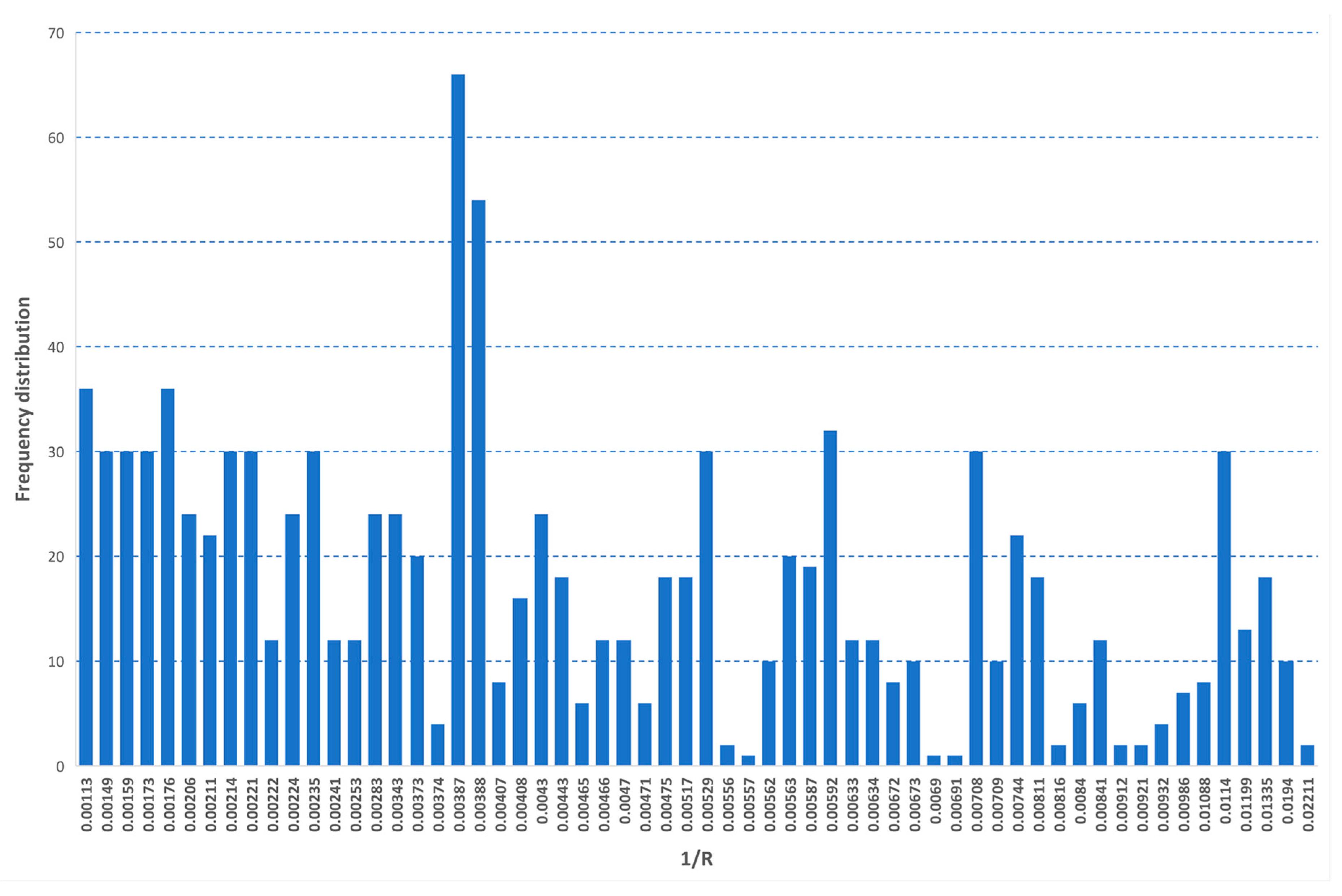
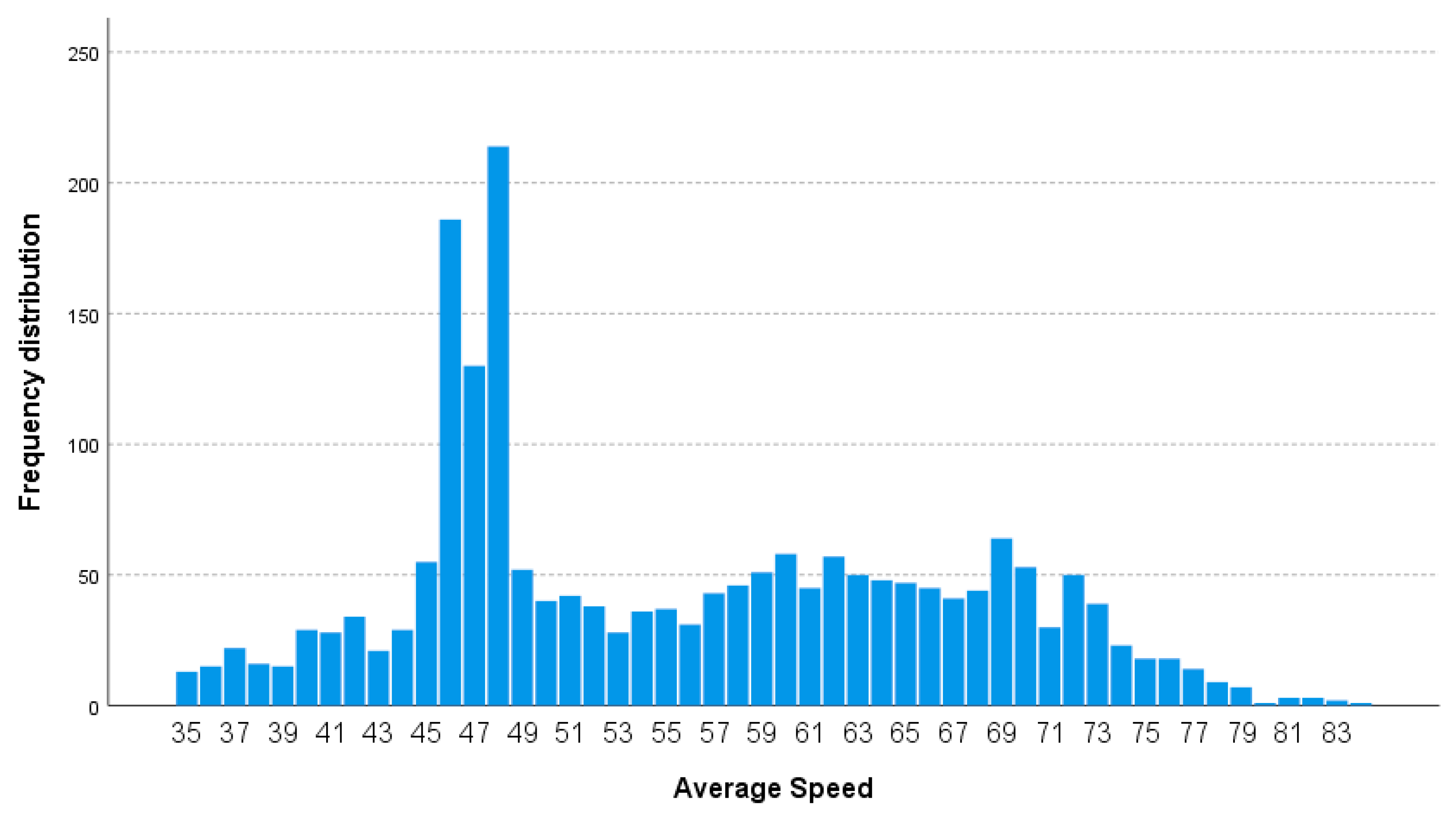
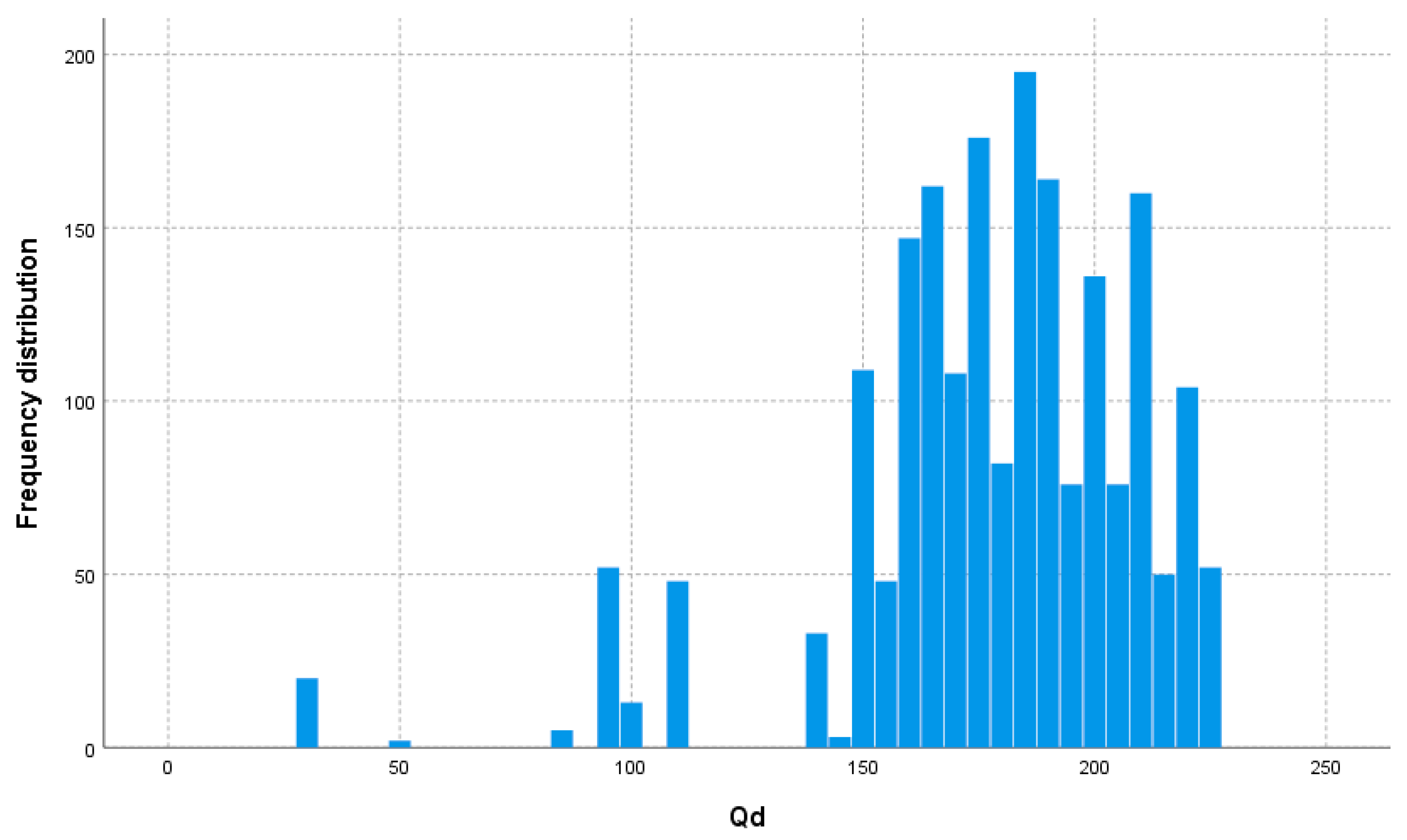
All the data collected during the experiment were referenced to homogeneous sections with a minimum and maximum length of 20 m and 74 m, respectively, characterized by a constant value for each variable. The minimum and maximum section lengths were defined to yield a traveling time between 1 and 6 s based on the range of running speeds. The dataset contained 1961 (97%) road sections without system fault (Lane Departure Warning LDW = 1) and 60 (3%) road sections with system fault (LDW = 0). The data do not have any missing values for all attributes. The summary statistics of the continuous variables in the database are reported in

Table 2. Summary statistics: continuous variables.

	N	Minimum	Maximum	Mean	Std. Deviation
1/R	2021	0.00000	0.0221	0.002427	0.0033032
Average speed (km/h)	2021	35	84	55.59	10.822
Qd	2021	30	223	178.10	32.548

and frequency distributions are shown Figure 2, Figure 3 and Figure 4. The data cover a wide range of values which are well distributed, as well.

We applied the CART algorithm to predict absence or presence of system fault based on values of the selected independent variables.

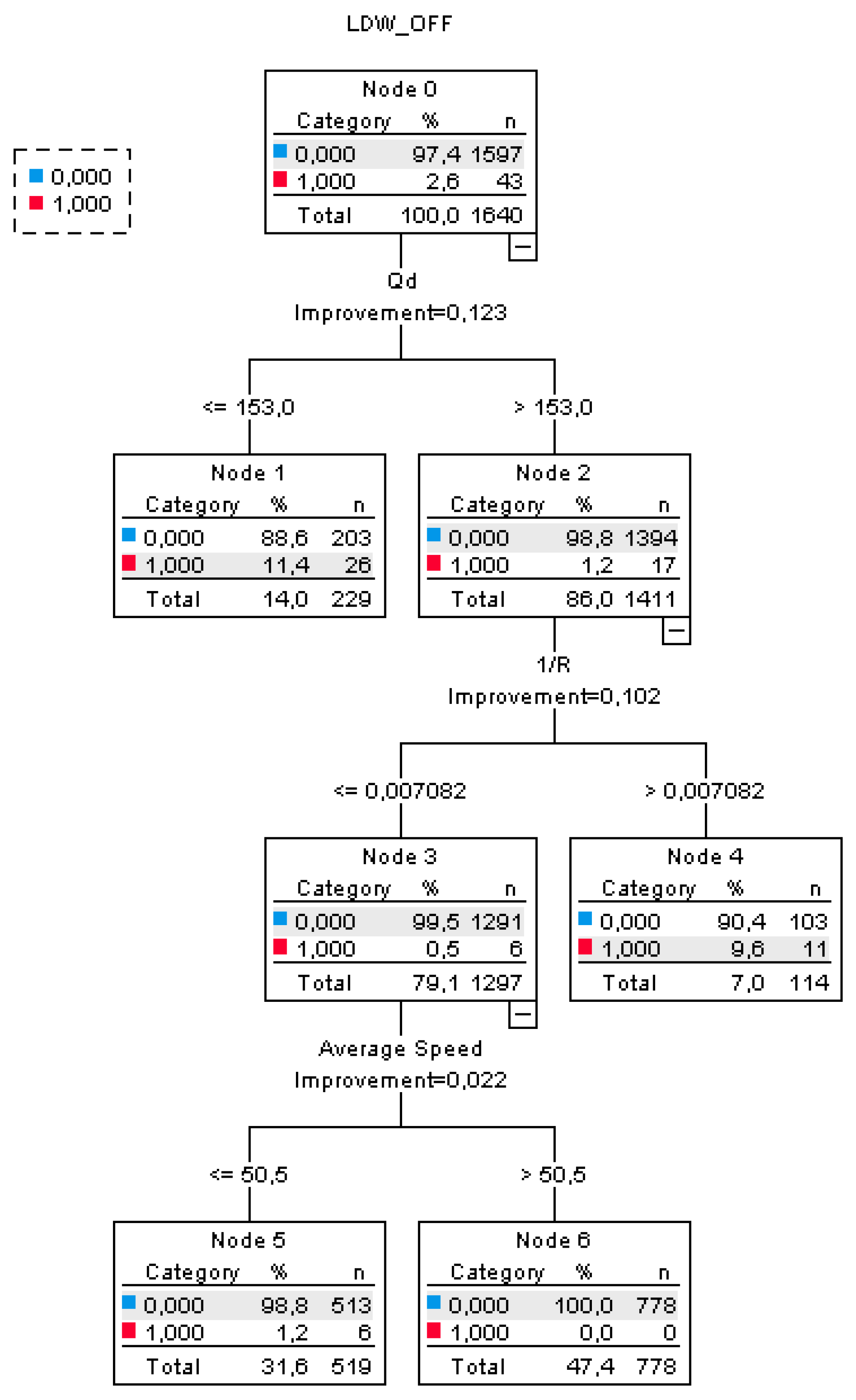
The database was randomly divided into two partitions with 80% of data for model calibration and 20% for validation. The tree diagram (Figure 5) shows the tree construction based on the calibration sample of 1640 cases (80% of the data), 0.0001 adjustments of the probabilities, a minimum parent node size of 200, a minimum child nodes size of 100 and equal misclassification costs. The Gini index was selected as a splitting criterion.

There were totally seven nodes that consist of four terminal nodes; the first node placed in the tree is the root node 0. The depth of the tree was equal to three. Parent node had 97.4% absence and 2.6% presence of the system fault.

To assess the performance of the models we applied measures of accuracy both to the calibration and validation data. A measure of the tree’s predictive accuracy is the risk estimate, that for categorical dependent variables, it is the proportion of cases incorrectly classified after adjustment for prior probabilities and misclassification costs [27]. In our study, the risk estimates results accurate with 16.6% (standard error 0.027) for the calibration sample and 19.0% (standard error 0.047) for the validation sample.

Another measure is the Percentage Correctly Classified which reached 81.0 per cent for the calibration and 79.8 per cent for the validation sample.

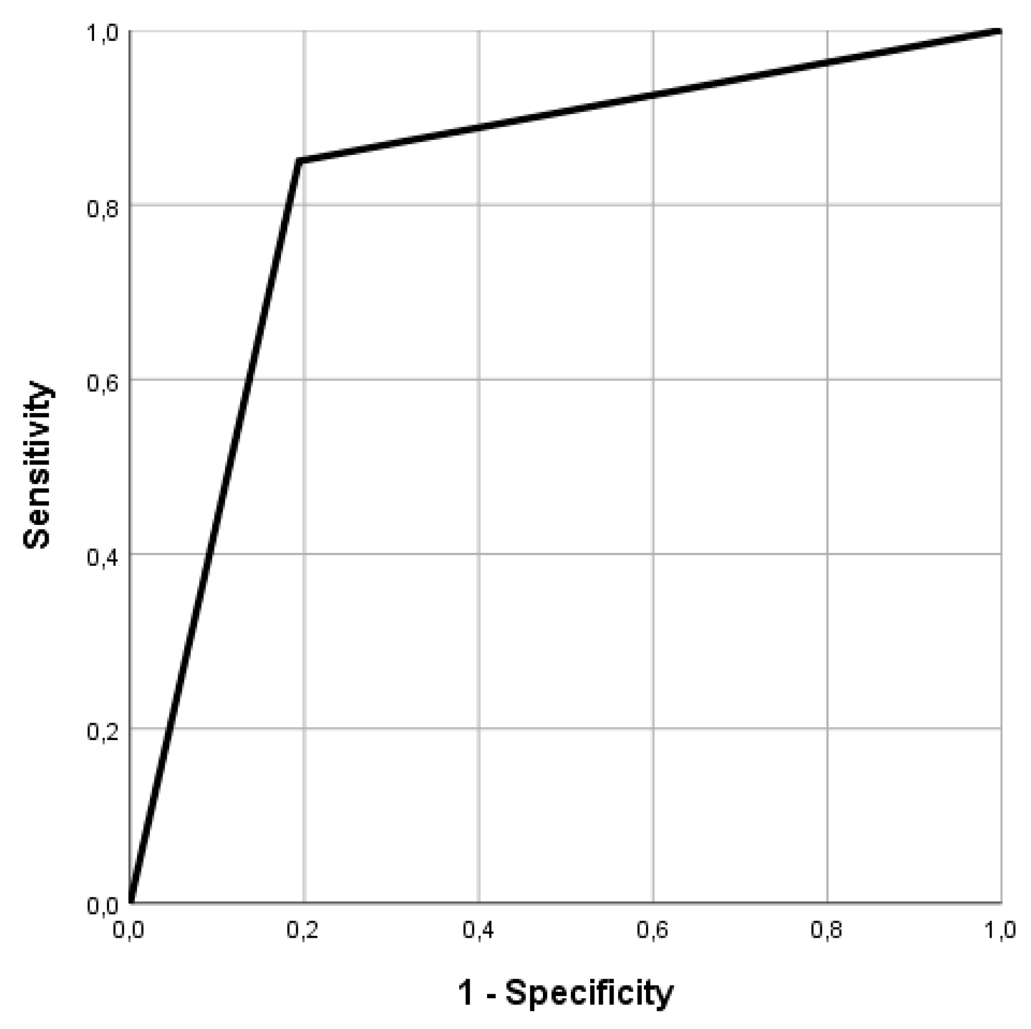
Finally, over the total sample size used, the prediction accuracy was 85% and the area under curve (AUC) was 0.828 (Figure 6) when a perfect diagnostic performance has an AUC equal to 1 [28].

The hierarchy of attributes in a decision tree reflects the importance of attributes. It means that the features on top are the most informative. The statistics shown in

Table 3. Summary statistics: continuous variables.

Independent Variable	Importance	Normalized Importance
1/R	0.127	100.0%
Qd	0.125	98.8%
Average Speed	0.048	37.9%

, measures importance of the variable by the increase of the effect of child node on the dependent variable. The importance is determined by the largest difference in the proportions of the dependent variable in the child nodes [29].

By analyzing the importance values, 1/R and Qd confirmed the meaningful contributes in the discrimination between the absence and the presence of system fault.

The first discriminator “Qd” has split the root node into two child nodes: Qd < 153 mcd/m²/lx (node 1, n = 285), and Qd > 153 mcd/m²/lx (node 2, n = 1736). The improvement for this classification was 0.123. If Qd is less than 153 mcd/m²/lx, the probability to have a fault rises to 11.4% for the calibration sample and 14.35 for the validation sample. Since it represents a terminal node, there is evidence that Qd value influenced the fault of the LSS system.

In the other branch of the tree, where Qd is more than 153 mcd/m²/lx, the system fault is influenced by the presence of a curvature radius less than 141 m (i.e., 1/R > 0.007082). The improvement for this classification was 0.102 and the probability to have a fault rises again to 9.6% for the calibration sample and 18.8% per the validation sample. Therefore, there is a clear evidence that curve with R < 141 m showed a higher percentage of faults than the average 3% in the test conditions.

The last split for Average speed has not produced further significant improvements because both the speed classes in the last node showed LSS fault percentages less than the average. Therefore, speed in the test conditions has not showed effects on LSS performance.

The results about Qd > 153 mcd/m²/lx for a fault probability of only 1.2% are more conservative than in other studies. In [30], Qd needs to be at least 85 while the NCHRP 20–102 project [31] figures out that for daytime dry conditions, Qd more than 100 seems appropriate. Anyway, the value of 153 in the present study confirm a contrast ratio higher than 1/3 as needed for reliable lane detection.

Regarding to curvature radius, despite many manufacturers’ specifications note that curves in horizontal alignment affect performance of lane-keeping-assist/lane-departure warning functions, there is limited quantitative analysis of the potential impact of curve radius. Sternlund observed that a small curve radius will affect machine vision enabled Lane Keeping Assist (LKA) functions [32].

It is worthily to mention that, based on data collected in the present study, we identified a 0% of LSS fault probability only for Qd > 153 mcd/m²/lx and R > 141 m at a speed higher than 50 km/h in daylight conditions.

6. Conclusions

Road departure is one of the main causes of single vehicle and frontal crashes accounting for more than one third of total road crashes. Typical accidents are normally occurring due to unintentional lane departure where the driver drifts towards and across the edge line of the lane.

In automated vehicles, several sensing methods are used for lane understanding and navigation including vision (video camera), LIDAR, RADAR, and Geographic Information Systems (GIS)/Global Positioning Systems (GPS)/Inertial Measurement Unit (IMU). Vision is the most prominent and ready to be applied because markings are already made for human vision, while LIDAR and GPS are important complements. The Lane Support Systems (LSS) uses cameras to “read” the line markings on the road and alert the driver if the car is approaching the lines. Machine vision technology used in these systems must rely on the same visual cues as human drivers such as road boundaries, road color and texture, and lane marking color and type.

In such framework, the paper presents an experimental study with a real-world data collection of LSS faults in different road characteristics and maintenance conditions.

The CART classification tree was selected to account for the sample size (2021 sections) with low probability of fault (3%) and quantitative explanatory variables.

CART confirmed marking quality and curvature radius as the most important factors to explain the LSS fault in the experimental conditions and road data sample. Threshold values have been identified, as well. The split discriminator value in the decision tree of Qd = 153 (mcd/m²/lx) is close to the minimum value usually requested for maintenance treatments and human vision requirements even if it is not unusual to have lower values in the road network in operation. Less documented is the actual limitation related to the horizontal curve radius. The threshold of R > 141 m and Qd > 153 provided a quantitative reference value with LSS fault probability equal to 0%.

Although the probabilistic form of logistic regression applied in a previous study [7] is more adapted to test variability in the system response, the classification CART resulted more intuitive and easier to interpret and estimate the frontiers nonparametrically.

A potential issue of the decision tree is its non-parametric nature and the limited capacity to account for unobserved heterogeneity [33]. Anyway, in our study, the issue of unobserved heterogeneity can be considered limited as the collected data come from a controlled experiment (e.g., free-flow, weather conditions, and driving behavior) and the database was cleaned from false positive and false negative due to artefacts (e.g., dust, parked vehicle, and marking discontinuities) [7]. Furthermore, the data analyzed is the response of a digital system for which random variability can be considered limited.

The lessons learned from this study can be used to apply the experimental approach to collect more extensive database to be analyzed with more advanced statistical models. The first opportunity of extension concerns the environmental conditions with the inclusion of different weather (e.g., rain) and lightning conditions (e.g., night). With databases of extended size and complexity, to account for the theoretical limitations of the decision tree (e.g., non-parametric nature, and unobserved heterogeneity) a “latent classes” approach can be applied combining CART to identify groups of observations with homogeneous variable effects within each group and logistic multilevel models to test the statistical correlations in longitudinal studies. Moreover, the identification of threshold values to define the Operational Design Domain of LSS may take into account higher cost on false negatives in future studies since failing of LSS may lead to serious consequence especially at automation levels higher than two.