Abstract
With rapid urbanization in China, the dramatic land-use changes are one of the most prominent features that have substantially affected the land ecosystems, thus seriously threatening sustainable development. However, current studies have focused more on evaluating the economic efficiency of land-use, while the loss and degradation of ecosystem services are barely considered. To address these issues, this study first proposed a land use-based input–output index system, incorporating the impact on ecosystem services value (ESV), and then by taking 30 provinces in China as a case study. We further employed the super-efficiency slacks-based model (Super-SBM) and the Stochastic Impacts by Regression on Population, Affluence and Technology (STIRPAT) model to explore the spatial–temporal changes and driving factors of the evaluated land-use eco-efficiency. We found that the evaluated ESV was 28.09 trillion yuan (at the price of 2000) in 2015, and that the total ESV experienced an inverted U-shaped trend during 2000–2015.The average land-use eco-efficiency exhibited a downward trend from 0.87 in 2000 to 0.68 in 2015 with distinct regional differences by taking into account the ESV. Our results revealed that northeastern region had the highest efficiency, followed by the eastern, western, and central region of China. Finally, we identified a U-shaped relationship between the eco-efficiency and land urbanization, and found that technological innovation made great contributions to the improvement of the eco-efficiency. These findings highlight the importance of the ESV in the evaluation of land-use eco-efficiency. Future land development and management should pay additional attention to the land ecosystems, especially the continuous supply of human well-being related ecosystem services.
1. Introduction
Ecosystem services (ES) are goods and services that are directly or indirectly related to human well-being and sustainability, and the supply of ecosystem services is subject to specific land-use structures and patterns [1]. However, emerging evidence shows that land-use changes can make fundamental impacts on ecosystem services provisioning [2]. It has been estimated that the global loss of ES value (ESV) can reach 4.3–20.2 trillion USD/year due to the land-use change [3]. A significant decline in global loss of ES value is also reported in China, which is 4.18–91.09 billion USD from 1988 to 2008 [4]. Moreover, in a small region of Nigeria, land-use changes led to a 4.83% decline in total ESV during 2000–2010 [5]. Facing this increasingly worsening situation, it has great significance to enhance the sustainable development through considering the ESV losses.
In principle, expansion of built-up land would change local land-use structures and patterns, thus directly affecting the supply of ES. For example, the heavy use of cultivated land will exert direct impacts on food production [6,7]. On the other hand, the land-use changes can strongly affect local climatic conditions [8], resulting in indirect responses of ESV to land-use changes, such as biodiversity loss [9]. Therefore, the trade-off between economic benefits and ESV losses needs to be addressed in the process of rapid urbanization. The dissection of the trade-off can provide important clues for sustainable development [10,11]. Currently, scholars have conducted a lot of meaningful work to ease this trade-off. For example, payments for ecosystem services (PES) is recommended as an efficient economic tool that can internalize the ecological cost into specific policy making [12]. In addition, economists are trying to construct a framework of the System of Environmental and Economic Accounting (SEEA), which can provide valuable information for sustainable policy-making [13].
In the process of urbanization in China, there are many issues associated with land-use, such as disordered exploitation, leave unused, low land-use efficiency, and so on [14,15]. Intensive land-use has been considered as an effective way to improve land-use efficiency. In general, high land-use efficiency means more economic benefits with less inputs per unit area [16]. The economic output per unit area has been used to represent land-use efficiency [17]. More generally, the non-parametric model, slacks-based model (SBM), is frequently applied to evaluate land-use efficiency [18,19,20]. In SBM, the scientific construction of an input–output index system is the premise of evaluating efficiency reasonably. The increasing environmental problems have led to extensive studies on evaluating the eco-efficiency of land-use in recent years [10,15,21,22]. Some undesirable outputs are considered in the efficiency evaluation, such as exhaust gas, waste water discharge, and solid waste discharge [10,15,21,22]. There is evidence that economic efficiency was higher than eco-efficiency when the undesirable outputs were taken into account. For example, after considering multiple undesirable outputs, including COD discharge, NOx, SO2, soot emission, dust emission, and industrial solid wastes, Zhang et al. [23] found that China’s average eco-efficiency was reduced to 0.39 from 0.50. Huang et al. [24] compared the results with and without undesirable outputs. They found that the average of eco-efficiency in China was reduced by 0.13 after considering COD, wastewater, exhaust gas, SO2, dust, solid waste, and smoke dust. These evidences highlight the importance of these undesirable outputs in the evaluation of eco-efficiency. However, the land-use change, especially in the context of rapid urbanization, exerts substantial impacts on provision of ES [2,3,4,5,25,26,27], seriously threatening the sustainable development. Therefore, it is necessary to incorporate the ESV impact into the evaluation of land-use eco-efficiency, otherwise, it may lead to unreliable conclusions [28].
Currently, Shi et al. [29] proposed a new eco-efficiency by dividing the economic output per unit area by the ESV per unit area. The use of this indicator has been reported to analyze the eco-efficiency changes from 2007 to 2015 in the case of Ningguo Gangkou industrial park in eastern China. However, this indicator cannot eliminate the influence of random factors, thus a comprehensive eco-efficiency indicator reflecting endogenous impacts should be provided. In addition, the eco-efficiency of provinces in China was evaluated in 2014 by a super-efficiency slacks-based model (Super-SBM), and the eco-efficiency in the most southeastern provinces was found to decline by taking into account the provincial aggregate ESV [28]. However, the variations of ESV are mainly driven by land-use changes, thus, considering the aggregated ESV in eco-efficiency calculation is unreasonable and unpersuasive in theory. In sum, current attempts to integrate the ESV into eco-efficiency still have some drawbacks. We attempt to make some improvements from the following three aspects: First, this study measures the eco-efficiency from the perspective of land-use change. Second, the spatial–temporal changes of the eco-efficiency are explored. Finally, we further analyze the driving factors of the eco-efficiency, which can provide more specific policy implications.
Finally, since the 1990s, China has undergone a remarkable urbanization and industrialization, and one of the most prominent features in this process is the dramatic expansion of built-up land [30]. As a valuable input factor, land resources are the basis of economic development, providing essential room for human activities and industrial organizations [31]. However, an extensive expansion of built-up land has also made substantial impacts on land-use patterns, such that a substantial amount of forest and cultivated land are encroached on during the rapid urbanization [25,26]. This deeply affects land ecosystems, thus hampering the continuous supply of ecosystem services [2]. Facing the increasing contradiction between economic expansion and land ecological conservation, it has great practical significance to evaluate and explore regional land-use eco-efficiency and its driving factors [15,32]. The main contents are organized as follows: We first introduced the data and the methods employed in this study. Then, the results were presented and analyzed, including the spatial–temporal variations of ESV and land-use eco-efficiency in China during 2000 to 2015, and the driving factors. The discussion, policy implication, and conclusion are given at the final part.
2. Data and Methodology
Based on previous studies, the present study made some extensions and improvements from the following aspects. First, we proposed a land use-based input–output index system, in which the ESV per unit of built-up land was considered. Second, the eco-efficiency changes over a long period from 2000 to 2015 in China were studied using the Super-SBM. Third, we further employed the Stochastic Impacts by Regression on Population, Affluence and Technology (STIRPAT) model to explore the driving factors of land-use eco-efficiency.
2.1. Data Sources
In this study, multisource data in different formats are used. Land use data at the resolution of 1 × 1 km2 covered 4 years (2000, 2005, 2010, and 2015), which were obtained from Resource and Environment Science and Data Center, Chinese Academy of Sciences (RESDC, http://www.resdc.cn/). In addition, net primary productivity (NPP), precipitation, and soil erosion data were used to calculate the ESV, which were also provided by RESDC. The socio-economic data were used to measure the driving factors of land-use eco-efficiency, which involved net profit per unit area of natural grain output (obtained from The Compilation of Cost and Income Data of National Agricultural Products), population, GDP, added value of secondary industry, and energy consumption (obtaining from China Statistical Yearbook). In addition, in order to eliminate the price effect, all currency data were converted to the price of 2000. Specifically, the consumer price index, fixed asset investment price index, and agricultural price index were applied to convert the price of GDP, fixed asset investment, and agricultural product to the price of 2000.
2.2. Dynamic Evaluation of ESV
2.2.1. Spatial–Temporal Adjustment of Equivalent Factors
The two prevailing methods are currently used to evaluate the ESV, namely equivalent factor method (EFM) and ecological modelling method (EMM), respectively [28,33]. EMM contains multiple parameters and complicated calculations, which are applicable to the ESV evaluation at local regions [33]. In contrast, EFM that requires less data and simple calculations is particularly suitable for the evaluation at large scale regions. Given this advantage, a large number of case studies based on EFM have been conducted in different regions, such as the global [3,34], China [4,33], India [35], Nepal [36], Nigeria [5], and so on. Therefore, in the present study, we applied EFM to evaluate the ESV in China.
The footstone of EFM is an equivalent factor for different ES functions. The seminal work by Costanza et al. provided an equivalent factor table for the global ecosystem [1]. For the terrestrial ecosystems in China, Xie et al. [33] have done extensive research in this area, and their findings provided the most comprehensive and solid equivalent factor table (Table 1). However, the equivalent factors in [33] are static, reflecting the average of a certain ES in a certain ecosystem [28]. In practice, ES provisioning is not only determined by land-use changes, but also subject to local natural and geographical conditions [37]. Based on previous studies [28,33,38,39], different ES functions are separately affected by critical ecological factors. In this study, we selected NPP, precipitation, and soil erosion level to realize spatial–temporal adjustment of the ES coefficients as described previously [33]. Specifically, the adjustment formula is given as follows:
where EFf is the equivalent factor value of ES function f in Table 1; Cijf is the adjustment coefficient for function f in province i and year j; is the adjusted equivalent factor value for function f in province i and year j. Function f = 1 refers to the function of FS, MS, GR, CR MSF, WT, BC, and CAS in Table 1, which is assumed to be linearly related to NPP. Similarly, function f = 2 refers to WS and WFR, which is assumed to be linearly related to precipitation, and function f = 3 refers to EP, which is assumed to be linearly related to soil erosion level. The formulas for adjustment coefficient Cijf are given as follows:

Table 1.
Table of equivalent factors for China’s terrestrial ecosystem provided by the reference [33].
- (1)
- Spatial–temporal adjustment coefficient of NPP:where NPPij is the NPP in province i and year j, and is the four-year average (2000, 2005, 2010, and 2015) of national NPP.
- (2)
- Spatial–temporal adjustment coefficient of precipitation:where Pij is the precipitation in province i and year j, and is the four-year average (2000, 2005, 2010, and 2015) of national precipitation.
- (3)
- Spatial adjustment coefficient of soil erosion level:where SEi is the soil erosion level in province i, it should be noted that soil erosion data are available merely for 1995 in this study, thus, is the average of national soil erosion level in 1995. According to RESDC’s classification, soil erosion is divided into 6 levels (from 1 to 6, the higher the value, the severer the erosion is). We applied the Zonal Statistics tool in ArcGIS 10.5 to calculate average erosion level as described in the literature [28].
2.2.2. Economic Value of Standard Equivalent Factor
We took the economic value of the average annual grain yield as a standard equivalent value. In this study, we included three main grain crops, namely rice, wheat, and corn. Furthermore, to eliminate the influence of human factors on grain output, we used the net profits of grain production to measure standard equivalent value. Finally, the value of standard equivalent factor can be obtained by the following formula:
where SEV is the calculated value of standard equivalent factor (yuan/km2). , and are the proportions of rice, wheat, and corn in their total cultivated area. , and are net profit per unit area of rice, wheat, and corn (yuan/km2), respectively. i is the year from 2010 to 2014. Agricultural price index r was used to convert the price in 2000. Finally, SEV was estimated at 1612.08 yuan/km2 at the price of 2000.
2.2.3. Evaluation of ESV
Finally, provincial and national ESV can be obtained by the following formulas:
where is the ESV in province i (yuan). is the area of land use type k in province i (km2). is the adjusted factor for function f of a certain land use type k in province i. is total ESV in China (yuan). m is the number of provinces.
2.3. Evaluation of Land-Use Eco-Efficiency
2.3.1. Input–Output Index System
The construction of the index system is the key to accurate evaluation of the land-use eco-efficiency. In this study, we selected capital stock per unit of built-up land (SCPBA), labor input per unit of built-up land (LIPBA), and energy consumption per unit of built-up land (ECPBA) as the inputs, meanwhile, pollutant discharge per unit of built-up land (PDPBA), GDP per unit of built-up land (GPBA), and ESV per unit of built-up land (EPBA) are taken as the outputs. In addition, due to the data availability, Tibet, Macao, Hong Kong, and Taiwan are not considered in this study. The specific data processing is described as follows:
- (1)
- SCPBA: This study employed perpetual inventory method to calculate the capital stock, and the formula is . Thereinto, is the capital stock in period t, which is made up of the fixed asset investment in period t and the depreciated value of cumulative investment in period t − 1. is the depreciation rate, which was provided by [40]. is the fixed asset investment in year t. The initial capital stock of each province in 2000 was estimated by [41]. Finally, the capital stock in 2000, 2005, 2010, and 2015 was determined by the formula of (n = 0, 5, 10 and 15).
- (2)
- LIPBA: Following [42], we used the total number of employees in each province to represent the labor input.
- (3)
- ECPBA: The total energy consumption represented as standard coal equivalent was used to measure energy input in each province [43].
- (4)
- PDPBA: This study selected sewage, exhaust, and solid waste to describe the undesirable outputs [24]. In addition, entropy method was used to obtain a single comprehensive environmental indicator [44].
- (5)
- GPBA: Routinely, the GDP of each province was used to describe the desirable output. The GDP was converted to the price of 2000 by the equation of . is the consumer price index in year i.
- (6)
- EPBA: Different from pervious researches, this study further considered the impact on ESV resulting from the land exploitation. Therefore, this study incorporated the ESV into the evaluation of land-use eco-efficiency.
It should be noted that all inputs and outputs mentioned above were divided by the area of built-up land in each province. By doing so, we can portray the land-use based production process. On the one hand, SCPBA, LIPBA, and ECPBA can reflect economic activity intensity. On the other hand, GPBA and PDPBA are used as the desirable and undesirable output, respectively. These two indicators have been routinely incorporated in traditional eco-efficiency evaluation [10,15,45]. Furthermore, the EPBA was also considered. To some extents, this indicator represents an ecological carrying capacity (ECC), the higher the indicator is, the better ECC is. In sum, on a comparable spatial unit, a region that consumes fewer resources, producing more desirable outputs, and simultaneously sustaining better ECC can be viewed as good performance, thus has higher land-use eco-efficiency. Table 2 shows the detailed description of the above variables.
Table 2.
The summary of the input–output indicators. SCPBA: Capital stock per unit of built-up land; LIPBA: Labor input per unit of built-up land; ECPBA: Energy consumption per unit of built-up land; PDPBA: Pollutant discharge per unit of built-up land; GPBA: GDP per unit of built-up land; EPBA: ESV (ecosystem services value) per unit of built-up land.
2.3.2. Super-SBM Model
SBM and stochastic frontier function (SFA) are two widely used methods for efficiency evaluation [46]. SBM is a non-parametric approach that can evaluate the efficiency of multiple decision making units (DMUs) with multiple inputs and outputs [47]. SFA needs to set up the production function in advance, which is more suitable for a large sample estimation [48]. In this study, we used a SBM model to evaluate the land-use eco-efficiency.
Traditional CCR model (developed by Charnes, Cooper, and Rhodes) evaluates the efficiency of a DUM between 0 to 1 [47]. The value of a DUM at the production frontier is equal to 1, and it can be considered efficient, while the DMU away from the frontier means that it is less efficient. A drawback of CCR model is that it cannot further distinguish the performances of the DMUs at the frontier. To address this issue, we applied an improved supper-efficiency model [49]. This method can be used to compare and distinguish the efficient DMUs. The higher the value of a DMU is, the better the efficiency is. In addition, the CCR model is a radial model, which cannot capture the slacks, resulting in overestimation of the efficiency [50]. Therefore, in the present study, we employed the Super-SBM model to evaluate the eco-efficiency. The Super-SBM model is given as follows:
where, we consider n DMUs with m inputs and s outputs. The vector form can be respectively expressed as . The matrices of and are defined as and . is a weighting factor, and and are the slacks of inputs and outputs. When , it means the evaluated DMU is less efficient, while means the DMU is efficient.
2.4. Influential Factor Analysis of Land-Use Eco-Efficiency
In order to explore the driving factors of the land-use eco-efficiency, this study used a widely accepted environmental attribution model, the STIRPAT model, to analyze the impacts of driving factors on land-use eco-efficiency. The general form of this model is shown as follows:
for the sake of reducing heteroscedasticity, we took the logarithm of formula (9), as follows:
where I is the environmental impact. P is the population. A is the wealth level. T is the technical progress. C is the constant term. is the error term. In our case, the variable I refers to the land-use eco-efficiency. Moreover, we introduced the indicators of land urbanization and its quadratic term in our empirical model [51]. For the sake of robustness, we perform three empirical models, model (1–3), which are given as follows:
where LUEE is the calculated land-use eco-efficiency. PD refers to population density, which was calculated by dividing the total population by the total area. PGDP refers to GDP per capita. TEC was the technology level. Referring to previous studies [15], we used energy consumption per unit of GDP as a proxy for TEC. The lower the TEC is, the higher the technology level is. In addition, to explore urbanization impacts on land-use eco-efficiency, land urbanization (LU) was introduced, which was calculated by dividing the built-up land area by the total area. and are provincial and year effect, and is the error term. , , and are regression results. The descriptions of the variables are shown in Table 3.
Table 3.
The summary of the variables.
3. Results
3.1. Spatial–Temporal Changes of ESV
Figure 1 and Table 4 show the overall variations of the ESV in China. For temporal changes, during the whole study period, the ESV was reduced by 1.5 billion yuan. Specifically, the ESV increased during the period of 2000–2005. This is because multiple major ecological protection projects were implemented around 2000, such as Grain for Green Project and the Sloping Land Conversion Program [52]. A remarkable achievement is the continuous conversion from the unused land and cultivated land to the forest. The total ESV experienced dramatic declines during the following two periods of 2005–2010 and 2010–2015. With the acceleration of urbanization, the huge demand for built-up land resulted in rapid loss and degradation of the natural or semi-natural land [39]. On average, the eastern and central region presented a similar inverted U-shaped trend (Table 4), while the western region maintained a growth trend across the whole period, demonstrating that the ecological protection projects are well effective in the western area [52]. However, the northeastern provinces experienced a significant decrease from 1864.20 billion yuan in 2000 to 1853.81 billion yuan in 2015.
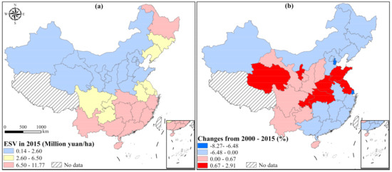
Figure 1.
The spatial distribution of ESV in 2015 (a); and the temporal changes of ESV during 2000–2015 (b).
Table 4.
Changes in ESV from 2000 to 2015 in different regions (billion yuan).
For spatial distribution, benefitting from the vast forest cover, the southern and northeastern areas presented high ESV per unit area (Figure 1). Fujian, Zhejiang, and Guangdong were the highest provinces with 11.76 million yuan/ha, 10.16 million yuan/ha, and 9.99 million yuan/ha, respectively. While the northwestern five provinces had the lowest value, specifically referring to Xinjiang (0.15 million yuan/ha), Ningxia (0.52 million yuan/ha), Qinghai (0.62 million yuan/ha), Gansu (0.78 million yuan/ha), and Inner Mongolia (1.00 million yuan/ha). This is because these areas are dominated by low ecological value land, such as the Gobi desert, bare land, degraded grassland, etc. In addition, the northern and southeastern provinces presented a declining trend, such that Tianjin and Shanghai exhibited the most declines, with the decline by 8.27% and 6.48%, respectively. Most of the growth was found in the Midwest. Shandong, Henan, and Ningxia increased the most, with the increase by 2.90%, 2.75%, and 2.02%, respectively.
3.2. Analysis of Land-Use Eco-Efficiency
3.2.1. Spatial–Temporal Changes of Land Use Eco-Efficiency
We selected SCPBA, LIPBA, and ECPBA as the inputs, and PDPBA, GPBA, and EPBA as the outputs. The Super-SBM model was used to calculate provincial land-use eco-efficiency. The detailed results are given in Table 5, and the spatial–temporal distributions are presented in Figure 2.
Table 5.
Land-use eco-efficiency changes of provinces from 2000 to 2015.
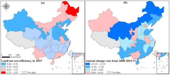
Figure 2.
The spatial distribution of land-use eco-efficiency in 2015 (a); and the temporal changes of land-use eco-efficiency during 2000–2015 (b).
Our results showed that the average of land-use eco-efficiency in China was 0.68 in 2015. From the perspective of the four regions, the northeastern region was the highest (1.05), then followed by the eastern region (0.70), the western region (0.64) and the central region (0.56) (Table 5). Specifically, Heilongjiang had the highest value of 1.87 in 2015, followed by Yunnan (1.21), Tianjin (1.17), and Beijing (1.16). Conversely, Shandong was evaluated as the lowest of 0.04, Hebei (0.10), Jiangsu (0.11), and Henan (0.13) were also at the bottom of the evaluated provinces. For spatial distribution (Figure 1a), in the southeastern region, only Beijing, Tianjin, Shanghai, Guangdong, and Hainan presented high land-use eco-efficiency. Previous studies have shown a gradual decline trend from the east to the west in China [24]. However, after considering the ESV, low values were found in the North China Plain and the northwest region (Figure 1a). This is because these areas are dominated by low ecological value land, such as the desert and cultivated land.
From the perspective of temporal changes, China’s land-use eco-efficiency presented a downward trend during 2000–2015. As shown in Table 5, the average land-use eco-efficiency in China was 0.87 in 2000, and dropped to 0.68 by 2015. The annual change rate during the period was −1.61%. Specifically, except for the northeastern region, the eastern, central, and western regions showed downward trends. For example, the western region had the highest drop (2.74%), followed by the eastern (1.33%) and central (0.99%) regions. As shown in Figure 2b, 9 provinces had experienced the growth. Of them, Ningxia increased the most by 14.81%, followed by Beijing (12.43%), Anhui (6.41%), Heilongjiang (2.88%), Jilin (1.07%), Tianjin (0.97%), Sichuan (0.54%), Guangdong (0.31%), and Yunnan (0.16%). These provinces had at least one prominent feature: The rapid economic growth or the ESV growth. These results confirmed the importance of ESV in the evaluation of eco-efficiency.
3.2.2. Comparison of Land Use Eco-Efficiency with and without ESV
As mentioned above, previous studies did not consider the ESV in the eco-efficiency evaluation, and this may lead to unreliable results. In the present study, we further analyzed how the eco-efficiency was affected by ESV.
Figure 3 presents the rank changes of the provinces in 2015 with and without ESV. In general, southwestern areas in China showed positive changes, while most provinces in the northeast had negative changes. Specifically, Yunnan and Guizhou experienced a significant increase of their ranks, from 22th and 26th to 2th and 15th, respectively. Because of their high EPBA, the EPBAs of Yunnan and Guizhou were 1001.55 million yuan/ha and 624.19 million yuan/ha, which were the two highest provinces. In other words, the ECC levels in these two provinces were relatively high. Besides the two provinces, the ECC levels in Chongqing, Sichuan, and Jiangxi also showed substantial improvements. On the contrary, the rankings of Henan, Gansu, and Xinjiang were found to reduce by 16, 11, and 9, respectively. The EPBAs of the three provinces were 15.23 million yuan/ha, 71.28 million yuan/ha, and 37.10 million yuan, respectively. It can be seen that these provinces had relatively poorer ecological conditions.
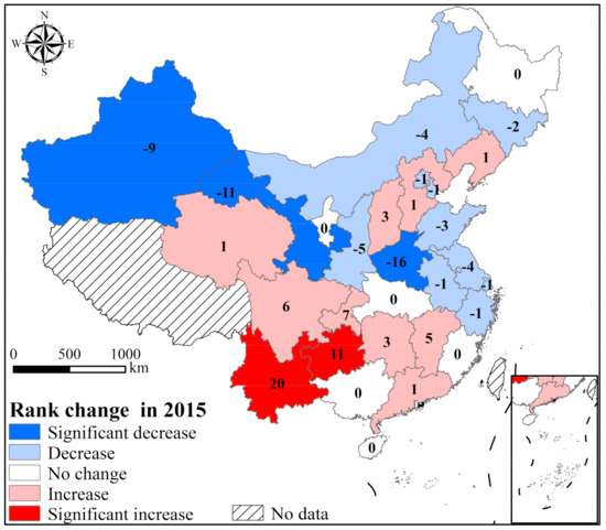
Figure 3.
The rank change of land-use eco-efficiency in 2015 with and without ESV.
To further explore policy implications, the slacks of the inputs and outputs were given in Table 6. First, we can observe that the proportion of total slacks in EPBA was the most, reaching 103.02%. It has been suggested that the loss and degradation of ESV are an unneglected problem in eco-efficiency evaluation. According to the average of four regions, western and central provinces exhibited higher shortages, which is mainly determined by the vast low-value land type cover in these provinces. In addition, the proportion of GPBA was the lowest due to the rapid economic development, resulting in the excess production [53]. Finally, the proportions of the three inputs were basically the same. However, the inputs in the central, western, and northeastern regions were significantly higher than those in the eastern region, suggesting that the excess investments in the midwestern area resulted in a certain level of production inefficiency [54].
Table 6.
The slacks of four regions in China for 2015.
3.3. Influential Factors of Land-Use Eco-Efficiency
First of all, according to the results of Hausman Test, we applied a fixed effect model to analyze the influential factors of land-use eco-efficiency. Based on the results of Table 7, the monomial term was negative, and the quadratic term was positive. This means that the relationship between land urbanization and land-use eco-efficiency follows a “U” shaped curve. This is due to extensive and inefficient exploitation resulting from the initial phase of urbanization, the unregulated, unordered, and blind urban expansion. However, with the continued urbanization, the government and the public have focused more on the quality of urban development [51]. For example, green infrastructures are planned and constructed during urban expansion, and the encroachment on natural and semi-natural land is strictly prohibited [51]. Moreover, the turning point of the “U” shaped curve was 1.47%, which has been achieved in 33 provinces in 2015. In addition, the GDP was a critical input in the evaluation of eco-efficiency, meanwhile, the per capita GDP was taken as a potential driving factor for the eco-efficiency variations. This treatment may result in biased estimation problem. Thus, for the sake of robustness, we selected another indicator of per capita income as the proxy in our empirical model. Results are shown in model (4) (Table 7), we can find that the basic results were unchanged, indicating that the estimation results were robust.
Table 7.
Regression results for driving factors of land-use eco-efficiency.
Regarding other driving factors, the population density and GDP per capita were positive (Table 7). However, only GDP per capita was significant, with the coefficient of 1.51. With the economic development, the improvements of production and energy efficiency as well as industrial structure lead to the promotion of eco-efficiency [51]. The coefficient of the technology level was negative (Table 7). In our study, we found that every 1% increase in the technology level can bring an increase in eco-efficiency by 0.54%.
4. Discussion and Policy Implication
Due to the rapid urbanization, the loss and degradation of ES has become an urgent problem. However, there is still a lack of effective methods to guide sustainable development. This study proposed a land use-based input–output index system, which incorporated the important ecological factor of ESV, and further, by employing the Super-SBM and STIRPAT model, we calculated and explored the spatial–temporal changes and driving factors of this creative eco-efficiency.
In the present study, we evaluated the ESV in China from 2000 to 2015. We found that the evaluated ESV was 28.09 trillion yuan (at the price of 2000) in 2015. One important finding in the present study is that only the western region exhibited a steady growth during the 15 years, while the eastern, central, and northeastern regions showed dramatic declines after 2005 according to the spatial–temporal changes in ESV. On the one hand, our results demonstrated that the major ecological protection projects were highly effective in the western region, e.g., the Grain for Green Project. On the other hand, rapid urban expansion in the mid-eastern region has encroached on a great deal of natural or semi-natural land, resulting in significant declines of the ESV in these areas. Therefore, in the future, more ecological conservation projects should be initiated and strengthened in the western region [52], and further extended to the mid-east. Moreover, strict restrictions on protection of cultivated land and urban development should be implemented, especially in central eastern areas.
The land-use eco-efficiency in China’s provinces during 2000–2015 was calculated based on the built land use-based input–output index system. A downward trend in eco-efficiency was identified. This result differed from most previous studies in which an upward trend in eco-efficiency in recent years has been reported [24]. We demonstrated that the ESV has considerable impacts on the evaluation of land-use eco-efficiency (Table 5 or Figure 2). Land-use change is one of the most prominent features of urbanization, which directly or indirectly affects the supply of ecological service. Therefore, the consideration of the ESV is highly essential when evaluating regional land-use eco-efficiency. In addition, an interesting finding is that some provinces with declining ESV showed eco-efficiency improvement. Beijing, Tianjin, and Shanghai were typical examples (cf. Figure 1b and Figure 2b). Due to the remarkable economic growth in these provinces, the contribution of economic growth outweighs the ESV losses, thus leading to an upward trend in eco-efficiency. However, it is worth noting that these provinces may be over-consuming local natural resources, hence, the total scale of built-up land should be strictly controlled, and more green infrastructures and ecological lands should be provided during urban development.
Finally, we further explored the driving factors of land-use eco-efficiency using the STIRPAT model. Our results indicate a “U” shaped relationship between land-use eco-efficiency and land urbanization in China. The improvement of the eco-efficiency may result from the intensive land-use and/or an increase in green infrastructure, as well as the extensive economic growth. Therefore, the underlying causes of this relationship need to be explored in the future. For policy makers, optimizing the spatial structure, promoting orderly development, and investing in green infrastructure are very important for sustainable urban development. In addition, the government should continue to strengthen its investment in the technology, especially in the field of green-oriented technological innovation [55].
5. Conclusions
This study evaluated the land-use eco-efficiency of China’s provinces from 2000 to 2015. By incorporating the ESV into the input-output index system, we explored spatial-temporal changes of the comprehensive land-use eco-efficiency, which could better reflect regional sustainability level. A Super-SBM model was applied to measure the efficiency, and then a panel STIRPAT model was employed to explore the driving factors of the efficiency. The results showed that the overall ESV experienced an inverted U-shaped trend during 2000–2015, but with obvious regional differences. In the eastern and central regions, they had a similar inverted U-shaped trend, while the western and northeastern regions presented a steady upward and downward trend, respectively. In addition, after incorporating regional ESV, the evaluated land-use eco-efficiency declined from 0.87 in 2000 to 0.68 in 2015. For spatial distribution, the eco-efficiency of the northeastern region was the highest, followed by the eastern region, the western region, and the central region. Finally, the results of the STIRPAT model indicated a U-shaped relationship between land-use eco-efficiency and land urbanization, and a significant improvement of the eco-efficiency by the technological innovation. These findings indicate that ecosystem services are important determinants for regional sustainable development. Therefore, land development should pay additional attention to the land ecosystems, especially the closely related provisions of ecosystem services.
Author Contributions
Conceptualization, Y.L. and C.W.; methodology, L.S.; formal analysis, H.S.; writing—original draft preparation, Y.L.; writing—review and editing, H.W., Z.X., X.Q., H.C., Y.X. and Y.W.; funding acquisition, C.W. All authors have read and agreed to the published version of the manuscript.
Funding
This research was funded by the Key Scientific and Technology Project of Inner Mongolia Science and Technology Department, grant number “2019GG012”, and the State Key Research and Development Program of China in the “13th 5-year Plan”, grant number 2016YFC0503402.
Data Availability Statement
Data available in a publicly accessible repository.
Conflicts of Interest
The authors declare no conflict of interest.
References
- Costanza, R.; D’Arge, R.; Groot, R.D.; Farber, S.; Grasso, M.; Hannon, B.; Limburg, K.; Naeem, S.; O’Neill, R.V.; Paruelo, J.; et al. The value of the world’s ecosystem services and natural capital. Nature 1997, 387, 253–260. [Google Scholar] [CrossRef]
- Hasan, S.S.; Zhen, L.; Miah, M.G.; Ahamed, T.; Samie, A. Impact of land use change on ecosystem services: A review. Environ. Dev. 2020, 34, 100527. [Google Scholar] [CrossRef]
- Costanza, R.; de Groot, R.; Sutton, P.; van der Ploeg, S.; Anderson, S.J.; Kubiszewski, I.; Farber, S.; Turner, R.K. Changes in the global value of ecosystem services. Glob. Environ. Chang. 2014, 26, 152–158. [Google Scholar] [CrossRef]
- Song, W.; Deng, X. Land-use/land-cover change and ecosystem service provision in China. Sci. Total Environ. 2017, 576, 705–719. [Google Scholar] [CrossRef]
- Arowolo, A.O.; Deng, X.; Olatunji, O.A.; Obayelu, A.E. Assessing changes in the value of ecosystem services in response to land-use/land-cover dynamics in Nigeria. Sci. Total Environ. 2018, 636, 597–609. [Google Scholar] [CrossRef]
- Power, A.G. Ecosystem services and agriculture: Tradeoffs and synergies. Philosophical transactions of the royal society B. Biol. Sci. 2010, 365, 2959–2971. [Google Scholar] [CrossRef]
- Deng, X.; Huang, J.; Rozelle, S.; Zhang, J.; Li, Z. Impact of urbanization on cultivated land changes in China. Land Use Policy 2015, 45, 1–7. [Google Scholar] [CrossRef]
- Costa, M.H.; Pires, G.F. Effects of Amazon and Central Brazil deforestation scenarios on the duration of the dry season in the arc of deforestation. Int. J. Climatol. 2010, 30, 1970–1979. [Google Scholar] [CrossRef]
- Pereira, H.M.; Navarro, L.M.; Santos-Martins, I. Global biodiversity change: The bad, the good, and the unknown. Annu. Rev. Environ. Resour. 2012, 37, 25–50. [Google Scholar] [CrossRef]
- Bryan, B.A.; Crossman, N.D.; Nolan, M. Land eco-efficiency: Anticipating future demand for land-sector greenhouse gas emissions abatement and managing trade-offs with agriculture, water, and biodiversity. Glob. Chang. Biol. 2015, 21, 4098–4114. [Google Scholar] [CrossRef] [PubMed]
- Broadbent, S.; Cara, F. Seeking control in a precarious environment: Sustainable practices as an adaptive strategy to living under uncertainty. Sustainability 2018, 10, 1320. [Google Scholar] [CrossRef]
- Jones, K.W.; Powlen, K.; Roberts, R.; Shinbrot, X. Participation in payments for ecosystem services programs in the Global South: A systematic review. Ecosyst. Serv. 2020, 45, 101159. [Google Scholar] [CrossRef]
- Yang, Y.; Jia, Y.; Ling, S.; Yao, C. Urban natural resource accounting based on the system of environmental economic accounting in Northwest China: A case study of Xi’an. Ecosyst. Serv. 2021, 47, 101233. [Google Scholar] [CrossRef]
- Chen, M.; Liu, W.; Lu, D. Challenges and the way forward in China’s new-type urbanization. Land Use Policy 2016, 55, 334–339. [Google Scholar] [CrossRef]
- Zhao, Z.; Bai, Y.; Wang, G.; Chen, J.; Yu, J.; Liu, W. Land eco-efficiency for new-type urbanization in the Beijing-Tianjin-Hebei Region. Technol. Forecast. Soc. Chang. 2018, 137, 19–26. [Google Scholar] [CrossRef]
- Cao, X.; Liu, Y.; Li, T.; Liao, W. Analysis of spatial pattern evolution and influencing factors of regional land use efficiency in China based on ESDA-GWR. Sci. Rep. 2019, 9, 520. [Google Scholar] [CrossRef]
- He, S.; Yu, S.; Li, G.; Zhang, J. Exploring the influence of urban form on land-use efficiency from a spatiotemporal heterogeneity perspective: Evidence from 336 Chinese cities. Land Use Policy 2020, 95, 104576. [Google Scholar] [CrossRef]
- Huang, J.; Xue, D. Study on Temporal and Spatial Variation Characteristics and Influencing Factors of Land Use Efficiency in Xi’an, China. Sustainability 2019, 11, 6649. [Google Scholar] [CrossRef]
- Gao, X.; Zhang, A.; Sun, Z. How regional economic integration influence on urban land use efficiency? A case study of Wuhan metropolitan area, China. Land Use Policy 2020, 90, 104329. [Google Scholar] [CrossRef]
- Kuang, B.; Lu, X.; Zhou, M.; Chen, D. Provincial cultivated land use efficiency in China: Empirical analysis based on the SBM-DEA model with carbon emissions considered. Technol. Forecast. Soc. Chang. 2020, 151, 119874. [Google Scholar] [CrossRef]
- You, H.; Wu, C.; Lin, N.; Shen, P. Assessment of eco-efficiency of land use based on DEA. Trans. Chin. Soc. Agric. Eng. 2011, 27, 309–315. [Google Scholar]
- Deng, X.; Gibson, J. Sustainable land use management for improving land eco-efficiency: A case study of Hebei, China. Ann. Oper. Res. 2020, 290, 265–277. [Google Scholar] [CrossRef]
- Zhang, B.; Bi, J.; Fan, Z.Y.; Yuan, Z.W.; Ge, J.J. Eco-efficiency analysis of industrial system in China: A data envelopment analysis approach. Ecol. Econ. 2008, 68, 306–316. [Google Scholar] [CrossRef]
- Huang, J.H.; Yang, X.G.; Cheng, G.; Wang, S.Y. A comprehensive eco-efficiency model and dynamics of regional eco-efficiency in China. J. Clean. Prod. 2014, 67, 228–238. [Google Scholar] [CrossRef]
- Chen, W.; Chi, G.; Li, J. The spatial association of ecosystem services with land use and land cover change at the county level in China, 1995–2015. Sci. Total Environ. 2019, 669, 459–470. [Google Scholar] [CrossRef]
- Gomes, L.C.; Bianchi, F.J.J.A.; Cardoso, I.M.; Filho, E.I.F.; Schulte, R.P.O. Land use change drives the spatio-temporal variation of ecosystem services and their interactions along an altitudinal gradient in Brazil. Landsc. Ecol. 2020, 35, 1571–1586. [Google Scholar] [CrossRef]
- Wang, Y.; Zhang, S.; Zhen, H.; Chang, X.; Shataer, R.; Li, Z. Spatiotemporal Evolution Characteristics in Ecosystem Service Values Based on Land Use/Cover Change in the Tarim River Basin, China. Sustainability 2020, 12, 7759. [Google Scholar] [CrossRef]
- Xing, L.; Xue, M.; Wang, X. Spatial correction of ecosystem service value and the evaluation of eco-efficiency: A case for China’s provincial level. Ecol. Indic. 2018, 95(Part 1), 841–850. [Google Scholar] [CrossRef]
- Shi, Y.; Liu, J.; Shi, H. The ecosystem service value as a new eco-efficiency indicator for industrial parks. J. Clean. Prod. 2017, 164, 597–605. [Google Scholar] [CrossRef]
- Liu, Y.; Fang, F.; Li, Y. Key issues of land use in China and implications for policy making. Land Use Policy 2014, 40, 6–12. [Google Scholar] [CrossRef]
- Bai, X.; Chen, J.; Shi, P. Landscape Urbanization and Economic Growth in China: Positive Feedbacks and Sustainability Dilemmas. Environ. Sci. Technol. 2012, 46, 132–139. [Google Scholar] [CrossRef] [PubMed]
- Lambin, E.F.; Meyfroidt, P. Land use transitions: Socio-ecological feedback versus socio-economic change. Land Use Policy 2010, 27, 108–118. [Google Scholar] [CrossRef]
- Xie, G.; Zhang, C.; Zhen, L.; Zhang, L. Dynamic changes in the value of China’s ecosystem services. Ecosyst. Serv. 2017, 26, 146–154. [Google Scholar] [CrossRef]
- Sannigrahi, S.; Bhatt, S.; Rahmat, S.; Paul, S.K.; Sen, S. Estimating global ecosystem service values and its response to land surface dynamics during 1995–2015. J. Environ. Manag. 2018, 223, 115–131. [Google Scholar] [CrossRef] [PubMed]
- Talukdar, S.; Singha, P.; Mahato, S.; Praveen, B.; Rahman, A. Dynamics of ecosystem services (ESs) in response to land use land cover (LU/LC) changes in the lower Gangetic plain of India. Ecol. Indic. 2020, 112, 106121. [Google Scholar] [CrossRef]
- Baniya, B.; Tang, Q.; Pokhrel, Y.; Xu, X. Vegetation dynamics and ecosystem service values changes at national and provincial scales in Nepal from 2000 to 2017. Environ. Dev. 2019, 32, 100464. [Google Scholar] [CrossRef]
- Zhang, B.; Li, W.H.; Xie, G.D. Ecosystem services research in China: Progress and perspective. Ecol. Econ. 2010, 69, 1389–1395. [Google Scholar] [CrossRef]
- Costanza, R.; de Groot, R.; Braat, L.; Kubiszewski, I.; Fioramonti, L.; Sutton, P.; Farber, S.; Grasso, M. Twenty years of ecosystem services: How far have we come and how far do we still need to go? Ecosyst. Serv. 2017, 28, 1–16. [Google Scholar] [CrossRef]
- Xing, L.; Zhu, Y.; Wang, J. Spatial spillover effects of urbanization on ecosystem services value in Chinese cities. Ecol. Indic. 2021, 121, 107028. [Google Scholar] [CrossRef]
- Wu, Y.R. The role of productivity in China’s growth: New estimates. J. Chin. Econ. Bus. Stud. 2008, 6, 141–156. [Google Scholar] [CrossRef]
- Zhang, J.; Wu, G.Y.; Zhang, J.P. The estimation of China’s provincial capital stock: 1952–2000. Econ. Res. J. 2004, 10, 35–44. [Google Scholar]
- Yu, J.; Zhou, K.; Yang, S. Land use efficiency and influencing factors of urban agglomerations in China. Land Use Policy 2019, 88, 104143. [Google Scholar] [CrossRef]
- Peng, B.; Wang, Y.; Wei, G. Energy eco-efficiency: Is there any spatial correlation between different regions? Energy Policy 2020, 140, 111404. [Google Scholar] [CrossRef]
- He, J.Q.; Wang, S.J.; Liu, Y.Y.; Ma, H.T.; Liu, Q.Q. Examining the relationship between urbanization and the eco-environment using a coupling analysis: Case study of Shanghai, China. Ecol. Indic. 2017, 77, 185–193. [Google Scholar] [CrossRef]
- Chen, W.; Si, W.; Chen, Z.M. How technological innovations affect urban eco-efficiency in China: A prefecture-level panel data analysis. J. Clean. Prod. 2020, 270, 122479. [Google Scholar] [CrossRef]
- Moutinho, V.; Madaleno, M.; Macedo, P. The effect of urban air pollutants in Germany: Eco-efficiency analysis through fractional regression models applied after DEA and SFA efficiency predictions. Sustain. Cities Soc. 2020, 59, 102204. [Google Scholar] [CrossRef]
- Charnes, A.; Cooper, W.W.; Rhodes, E. Measuring the efficiency of decision making units. Eur. J. Oper. Res. 1978, 2, 429–444. [Google Scholar] [CrossRef]
- Liu, S.; Xiao, W.; Li, L.; Ye, Y.; Song, X. Urban land use efficiency and improvement potential in China: A stochastic frontier analysis. Land Use Policy 2020, 99, 105046. [Google Scholar] [CrossRef]
- Tone, K. A slacks-based measure of super-efficiency in data envelopment analysis. Eur. J. Oper. Res. 2002, 143, 32–41. [Google Scholar] [CrossRef]
- Tone, K. A slacks-based measure of efficiency in data envelopment analysis. Eur. J. Oper. Res. 2001, 130, 498–509. [Google Scholar] [CrossRef]
- Tang, M.; Li, Z.; Hu, F.; Wu, B. How does land urbanization promote urban eco-efficiency? The mediating effect of industrial structure advancement. J. Clean. Prod. 2020, 272, 122798. [Google Scholar] [CrossRef]
- Ouyang, Z.; Zheng, H.; Xiao, Y.; Polasky, S.; Liu, J.; Xu, W.; Wang, Q.; Zhang, L.; Xiao, Y.; Rao, E.; et al. Improvements in ecosystem services from investments in natural capital. Science 2016, 352, 1455–1459. [Google Scholar] [CrossRef] [PubMed]
- Yang, Q.; Hou, X.; Zhang, L. Measurement of natural and cyclical excess capacity in China’s coal industry. Energy Policy 2018, 118, 270–278. [Google Scholar] [CrossRef]
- Wang, J.; Zhao, T.; Zhang, X. Environmental assessment and investment strategies of provincial industrial sector in China—Analysis based on DEA model. Environ. Impact Assess. Rev. 2016, 60, 156–168. [Google Scholar] [CrossRef]
- Wang, M.; Li, Y.; Cheng, Z.; Zhong, C.; Ma, W. Evolution and equilibrium of a green technological innovation system: Simulation of a tripartite game model. J. Clean. Prod. 2021, 278, 123944. [Google Scholar] [CrossRef]


Publisher’s Note: MDPI stays neutral with regard to jurisdictional claims in published maps and institutional affiliations. |
© 2021 by the authors. Licensee MDPI, Basel, Switzerland. This article is an open access article distributed under the terms and conditions of the Creative Commons Attribution (CC BY) license (http://creativecommons.org/licenses/by/4.0/).