Abstract
Bicycles-on-board (BoB) transit is a popular travel demand management (TDM) tool across many U.S. cities and universities, yet research on this mode within a university environment remains minimal. The purpose of this research is to investigate how personal and neighborhood factors influence this travel choice in a university setting. Relying on attitudinal data from a stated preference survey, this study examined the effect of personal characteristics and seven key neighborhood conditions on the willingness to utilize BoB for the “first mile” of the journey to campus. The study used exploratory spatial data analysis (ESDA), a discrete choice modeling framework, and geovisualizations to understand the likelihood of choosing this mode among a university population in Flint, Michigan, USA. The results revealed that the majority of constituents were not interested in BoB, aside from a cluster near the commercial business district. Also of note was that long commutes, and reduced access to parks and bicycle facilities dissuaded people from choosing this mode. Surprisingly, a neighborhood’s walkability or bikeability had no effect on respondent’s interest in using BoB. Lastly, the geovisualizations showcased where localized interventions may effectively increase this mode choice in the future.
1. Introduction
Cities across the globe face unprecedented growth due to urbanization. A large segment of society now live in urban areas [1], and, by 2050, 66% will reside in cities [2]. This statistic is concerning given that current urban mobility systems—which are largely dependent on the automobile—are untenable due to the lack of space, environmental externalities, inefficient energy use, and concerns over public health [3,4]. Thus, integrating public transit with emission-free transport modes, such as bicycling, remains critical for creating sustainable transportation systems that increase the quality of urban life.
Interest in combining travel modes among policy-makers is growing in light of global urbanization trends, infrastructure resilience fears, urban health concerns, and the need for promoting sustainable transportation systems [4,5,6,7]. The notion of creating sustainable transportation systems within cities and universities alike has been a goal for at least the last 25 years [8,9]. It has been posited that an important first step for creating such a system is to understand the ecology of transport modes. For instance, in many cities, a complex system of travel modes and infrastructures coexist (i.e., driving, transit, bicycle lanes, scooters, etc.), but rarely interact [6]. This undermines the full potential of creating a sustainable transportation system. Therefore, a better understanding of the relationship among different transportation systems is needed.
In recent decades, researchers and policy-makers have proposed ways to integrate bicycling and transit to ease transit access and egress conditions. The assimilation has several benefits; chief among them is that it enhances transit’s catchment area and adoption [10]. This is realized, through the combined short-distance travel-sheds and speed afforded by bicycling, with the long-distance travel capabilities of buses, rail, and other transit modes. Additionally, when bicycles are integrated with transit, they can promote livable communities, replace automobile trips, and elevate public health [11,12,13]. Common approaches to promote this integration have consisted of: innovative planning interventions, policy analysis, economic performance measurements, and educational programming [14,15,16,17,18]. Furthermore, assimilating bicycling and transit can occur in several ways: (a) ride and park near the transit stop, (b) sharing bicycle use (i.e., bicycle rentals), (c) integrated planning and operation, and (d) bicycles-on-board buses (referred to as “BoB” hereafter) and regulation [19]. The ability to bring bicycles on-board transit is a popular option among transit riders, transit agencies, and universities [8,15]. Approximately 72% of U.S. transit systems have bicycle racks installed on buses, thus making the BoB mode interventions the most popular strategy for increasing “first and last mile” transit access [20]. The “first and last mile” term has been coined by planners to describe the distances traveled before and after boarding transit [21]. Despite the popularity of BoB mode interventions in the U.S.—80–90% of transit trips start by either walking or bicycling—the relationship remains complex and poorly understood [15,22].
The viability of intermodal transport using BoB remains mixed. Previous research has shown that these systems are underutilized, delay transit, have limited rack capacity, and increase transit delays [19,23]. Research from Europe has indicated that carrying bicycles on board transit during peak times takes up space for others and may make other passengers uncomfortable [24]. Other studies show that BoB is increasing in use and popularity. Pucher [25] and Krizek et al. [15] highlighted a clear demand for BoB mode shares and Ensor et al. [26] indicated that cycle-transit use may provide substantial economic benefit for transit agencies. In contrast, much like people’s attitudes towards transit, negative sentiments also prevailed among cycle-transit users in a recent study conducted in Philadelphia [27]. BoB mode shares may also be a primary mobility option for those without low-income persons without automobiles [28] and university students [8]. Other related research has shown that the main predictors for this mode are trip distance, weather, and trip purposes [21,29,30]. What remains indeterminate is how personal and neighborhood conditions together may facilitate (or negate) this mode choice during the “first-mile”, especially in a university environment. This leaves us with an incomplete understanding of how to effectively elevate this mode, consequently reducing the full potential for universities, and their host cities, to reach their sustainability goals.
In recognition of this research need, the current study had two research objectives: (i) describe the travel behavior and preferences towards BoB mode choice among a university sample using empirical and exploratory spatial data analysis (ESDA), and (ii) implement a discrete choice modeling strategy, coupled with geovisualizations, to assess the probability of using BoB as a function of spatially varying personal and neighborhood conditions in the City of Flint.
2. Materials and Methods
2.1. Study Area and Context
The study area in this research is the City of Flint and the primary schools of higher education residing within (Figure 1). The city is the 7th largest in Michigan and has a population of 94,867. Recently, the city has begun to be known as a “college town” due to the presence of several colleges and universities. In this research, we focused on the largest three—The University of Michigan-Flint (UM-Flint), Mott Community College (MCC), and Kettering University (KU). UM-Flint is an urban campus, has a student enrollment of 7297, and is classified as a commuter campus [31,32]. Mott Community College is a 2-year public institution and recent enrollment estimates are 7715 [33]. Like UM-Flint, the College is a commuter campus and does not provide student housing. KU is a private university with an estimated enrollment of 2315 and contains several student dormitories [34]. The University is well-known for its engineering program and resident student population. All of the schools have made significant strides in promoting sustainable transportation and other “green” initiatives. For instance, UM-Flint has instituted a “Go Blue, Live Green” strategy and has partnered with local stakeholders to help implement a bicycle-share program [35], and, in 2013, the university was designated as a “bicycle-friendly university” by the League of American Cyclists [36]. KU has launched the “Generating Responsible Ecological & Environmental Neighbors (GREEN)” course cluster for all majors [37] and has recently installed a bike shop and mobile bike repair-stand on campus. MCC is also focused on promoting sustainable transportation by hosting bicycle education workshops for kids [38].
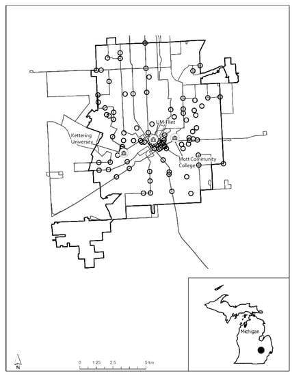
Figure 1.
Map of the City of Flint, MTA bus routes, university locations, and reported participant residences identified by the black circles.
2.2. Sample and Survey Instrument
The current study utilized a cross-sectional stated preference survey created in 2013 and administered by the MTA in Flint, Michigan. The survey was developed using Survey Monkey (www.surveymonkey.com), and a link was distributed to all faculty, staff, and students using email, university websites, and Blackboard learning software. The survey was made available from 15 October until 15 November 2013, with one reminder sent out during this time frame. Respondents from each university and college were asked questions regarding their demographics, transportation characteristics, bus usage, routes, destinations, vehicle and bicycle ownership, MTA pass ownership, BoB interest, home location, and attitudes about transit (n = 243 for UM-Flint; n = 180 for MCC; n = 61 for KU). The survey did not collect information on their university status (i.e., faculty, staff, or student). Notably, females were over-represented in the sample at 62.82% and younger persons (21–24) were the majority age group, representing 18.50% of the sample. Each participant was asked for their nearest home address or cross-street location, and zip code. This was used to geolocate each participant’s residence using GIS software. The spatial distribution of the sample, after removing erroneous records or missing data, was 138 (see Figure 1).
2.3. Data and GIS Measures
2.3.1. Survey Data
To measure the probability of choosing BoB mode share among the sample, we used the MTA survey question: “Would you utilize a rack on the bus for your bike?” The dichotomous response was used as the dependent variable in all models and coded 1—yes and 0—no by MTA staff.
Borrowing from past works on active travel correlates and the socioecological model [39,40], several independent variables were considered in this research and grouped based on personal and neighborhood conditions near each respondent’s residence (i.e., the first mile). The personal variables—demographics, travel behaviors, and attitudes—were mined from the survey. We focused on: gender, age group, university affiliation, auto-ownership, commute time, bicycle ownership, and MTA pass ownership. Answers to mode-choice decisions and perceived distance to bus stops were also considered, as attitudes towards travel conditions can affect travel mode decisions [41]. MTA staff coded all survey responses for this study.
2.3.2. Objective Neighborhood Conditions
To assess the influence of objective neighborhood conditions on the probability of using BoB, we evaluated numerous indicators pertaining to: accessibility, diversity, design, density, socioeconomic standing (SES), walkability/bikeability, and safety at the Census Block Group (CBG) scale. The majority of the factors were from national, state, and local government sources. The majority of the neighborhood factors were from the U.S. Environmental Protection Agency (EPA) Smart Location Database (SLD) version 2.0 (https://www.epa.gov/smartgrowth/smart-location-mapping). The database contains 90 different travel-related correlates drawn from the 2010 decennial Census and American Community Survey [42]. We also collected bicycle/pedestrian crash incidents and land-use GIS data from the State of Michigan for the year 2010; these metrics were used to assess active travel safety and land-use typologies, respectively. The City of Flint and Genesee County Land Bank provided several community attributes in a GIS-ready format, including: vacant housing, schools (K-12), parks, roadways, crimes (arson, murder, and theft), sidewalks, and bicycle facilities (on-street and off-street). These indicators accurately represented conditions at the time of survey dissemination. The MTA provided bus stops and bus routes from the year 2013 and were aggregated to CBG’s using spatial analysis. We normalized all point and line variables by CBG area (km) to minimize errors associated with the modifiable areal unit problem (MAUP). Destination accessibility is also important for bicycle and transit mode choices. While past research has shown that access varies by travel mode [43], other studies indicated that straight-line (i.e., Euclidian) distance is a suitable metric [44]. Thus, we used the latter technique to gauge each respondent’s accessibility to the closest park, bike facility (trail or on-street route), and bus stop. We also hypothesized that the walkability and bikeability within a neighborhood could affect intermodal transportation decisions. Therefore, we incorporated a national walkability index developed by the U.S. EPA (https://catalog.data.gov/dataset/walkability-index), where elevated values relate to increased walkability. Using Flint roadway data from 2012, we derived a common bicycle level of service (BLOS) index for each road in the city using the formula developed by Landis et al. [45]: reduced values equate to safer bicycling conditions. The mean value of each index was joined to the CBG’s using a point in polygon procedure in GIS. The final set of variables are shown in Table 1.

Table 1.
Descriptive statistics and definitions of dependent and independent variables, n = 138.
2.4. Empirical and ESDA Techniques
In regards to our first objective (i) in this study, an empirical analysis was implemented first to describe travel behavior trends. We then implemented two ESDA techniques to visualize the spatiality of BoB interest. First, kernel density “hot-spot” maps of each respondent’s interest (i.e., yes vs. no) in BoB were created. Kernel density maps are an established means to highlight the density of a spatial phenomenon as a raster surface. The quadratic kernel function—as described by Silverman [46]—was selected and implemented in GIS software to visualize the geography of BoB interest. To test this outcome statistically, we utilized a univariate join count statistic developed by Anselin et al. [47] to visualize significant clustering of interested BoB responses (i.e., “yes” choices). A pseudo p-value is derived using a conditional permutation approach for those values equaling 1. The GeoDa software (version 1.14) was implemented to compute the index, and we used GIS to create the visualizations.
The index takes the form:
where: xij is 1 and 0, and wij represents the not row-standardized spatial weights.
2.5. Global Discrete Choice Model Development
Discrete choice models have long been used to model travel behavior and land-use interactions [48]. Following this tradition, we implemented three discrete choice models in this study—two global and one spatial—to predict the odds of an event (i.e., a “yes” response to interest in BoB) to reach our second research objective (ii). When fitting logistic regression models, it is important to first examine the independent variables for multicollinearity. Testing for this where the maximum acceptable variance inflation factor (VIF) of 10 was held [49]. Additionally, we removed insignificant (p ≥ 0.05) factors and verified that the model assumptions were not violated. Next, the linearity between the dependent and independent variables using the Box–Tidwell [50] procedure was tested. Independent variables that were not found to be linearly related to the logit of the dependent variable were transformed using the natural log. To further verify the selected independent variables (see Table 2) were appropriate, the Hosmer–Lemeshow statistic was relied on. A non-significant value (p > 0.05) signifies that the independent variables are linearly related to the dependent variable [51].
Table 2.
Stated travel behaviors among the university sample, n = 139.
The global logistic regression (GLR) model is a probabilistic nonlinear regression model where the independent variables can either be continuous or discrete and do not need to have normal distributions [52]. The model produces a single coefficient of determination (R2) and single β coefficient for each covariate. It is assumed that the β and log-odds are constant throughout the study area, hence the probabilities are “global.” The resulting coefficients are interpreted as an odds-ratio (OR’s), with an OR above one indicating that the independent variable increases the likelihood of BoB interest, and an OR below one indicating that the independent variable decreases the likelihood of BoB interest. The first model (Model 1) in this study utilized a forward stepwise approach where the independent variables from Table 2 were entered and removed automatically based on statistical significance (p < 0.05). A second model (Model 2) was created where independent variables were simultaneously entered based on reduced VIF values (p < 0.05) and hypothesized relationship to the dependent variable. As a last measure of GLR model fit, a confusion matrix was created, where a greater number of correctly classified observations demonstrates a better fitting model. The GLR models were developed using IBM SPSS software (version 26).
2.6. Spatial Discrete Choice Model Development—GWLR
After creating the best fit GLR models, the standardized residuals for autocorrelation were tested using the Moran’s I statistic as suggested by Shaker [53]. Since a statistically significant (p < 0.05) index was found in the GLR (Model 2), a GWLR model was computed, making this the “spatial discrete choice” model (Model 3). The GWLR model is an extension of GLR in that it accounts for spatial dependency and spatial non-stationarity among variables [54,55]. Stated differently, the coefficient estimates vary for each observation (i) based on its geographic coordinates, thus building a local regression model for each dependent variable and selected independent variables within a neighborhood (i.e., kernel). The result is a refined model which produces multiple β coefficients for each observation in the sample.
The model is expressed formally as:
where: P(ui,vi) is the probability of choosing “yes” at point (ui,vi), β1(ui,vi), is the local coefficient of point (ui,vi), representing the local effect of influencing factors xi and β0(ui,vi) is the intercept of point (ui,vi).
To compare and contrast the three discrete choice models, we selected a golden search adaptive bandwidth kernel that minimizes the AICc (Corrected Akaike Information Criteria) for our GWLR model. The method prevents model over-fitting and provides an optimal bias-variance trade-off [56]. A model with a lower AICc is considered ideal. We also considered the pseudo R2 as a measure of model fit. Lower AIC values and higher R2 (i.e., percent deviance explained) indicate a stronger model. The GWLR model was created in GWR4 software, version 4.0.90 [55].
The optimal means to examine GWLR coefficients is through mapping [57] and since Model 3 is the most robust in this study, we mapped the statistically significant (p < 0.05) coefficients to visualize where the independent variables significantly influenced interest in BoB. This approach follows the methodology proposed by Matthews et al. [58] and highlighted in prior travel demand research [59].
3. Results
3.1. University Travel Characteristics
The first research objective “i” in this research was to empirically describe the sample population and geovisualize interest in BoB. Table 2 shows that personal automobile use dominates all trips to university, with those associated with UM-Flint the highest at 70.8%. The largest portion of people walking to school occurred at KU (29.5%). As for bus mode shares, 27% of MCC and 10% of UM-Flint respondents used this mode to reach the university. No respondents from KU reported using the bus to travel to school or otherwise. Respondents from KU also indicated that their university trips were short—68.9% reported a commute time was less than ten minutes. Commute times for respondents from UM-Flint and MCC were longer, ranging from 10–39 min. Except for the KU sample, most respondents did not have a bus stop within five minutes of their residence. Interest in the BoB mode choice was largely negative, regardless of university affiliation. Respondents from UM-Flint and Mott indicated that they would consider BoB nearly 40% of the time, while only 13.1% of those from KU said they would consider this mode. Considering the large percentage of drivers commuting to UM-Flint and MCC, and the elevated proportion of those who may consider BoB—when compared to KU—targeting, these populations may induce a mode shift to intermodal transportation.
3.2. Visualizing Interest in BoB
Figure 2 displays the respondents’ residences and their interest in BoB resulting from our ESDA approach. The kernel density maps (Figure 2a,b) depict the concentrations of respondents who were and were not interested in BoB. Generally, interest was concentrated near UM-Flint and the City’s commercial business district (CBD) (Figure 2a), whereas disinterest was located near KU and the CBD, which is consistent with our empirical findings displayed in Table 2 (Figure 2b). We found overlapping interest (yes vs. no) near the CBD, which is likely because these decisions were split between the UM-Flint and MCC sample (see Table 2), and those respondents may reside near one another. Figure 2c shows where statistically significant (p ≤ 0.05) clusters of individuals interested in BoB resided. The significant clusters were mainly located in-between KU and UM-Flint, and close to the CBD (Figure 2c). This outcome shows that the likelihood of using BoB travel mode is spatially clustered in areas where the commute time to university is reduced, meaning that BoB may not be a viable mode for those who live far from the University.
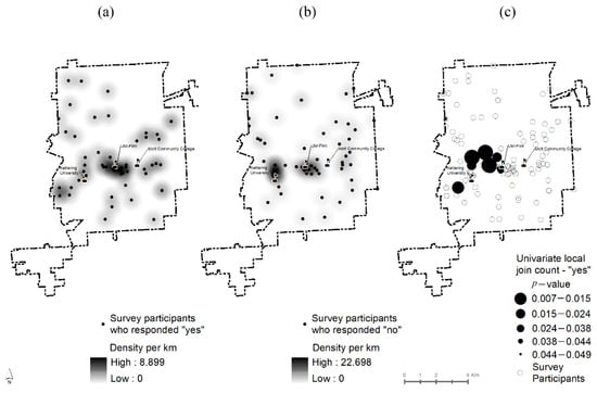
Figure 2.
Kernel density “hot-spots” of participants who indicated “yes” (a) and “no” (b) regarding BoB travel interest; statistically significant (p ≤ 0.05) clusters’ locations where participants said “yes” (c).
3.3. Global and Spatial Discrete Choice Model Diagnostics
The second objective (ii) of this research was to examine the personal characteristics and neighborhood conditions impacting interest in BoB. As previously described, we created three discrete choice models. In Table 3, the stepwise model is represented as “Model 1”; the simultaneous GLR model is “Model 2.” Due to residual autocorrelation in Model 2, we created “Model 3,” the spatial discrete choice model (GWLR), which, as previously mentioned, is novel in that it accounts for spatial autocorrelation. The diagnostics and coefficients from all three models are shown in Table 3. The fit statistics indicate that the selected independent variables were not co-linear and fit both GLR models well (VIF < 5.00, Hosmer–Lemeshow statistics p > 0.05). Of the two GLR models, Model 2 was the strongest. An increase in the psuedo R2 and decrease in AICc over Model 1 was observed, with values of 0.364 and 152.36, respectively. However, residual clustering was apparent (p < 0.05) based on the Moran’s I statistic; highlighting non-stationary OR’s (i.e., odds-ratios). The local Model 3 showed marginal improvement over Model 2. Entering the same independent variables as this model, the psuedo R2 and AICc values were 0.400 and 151.95, respectively. This improvement over Model 2 indicates a stronger model when spatiality is accounted for. Lastly, the Moran’s I analysis of standardized residuals showed no significant signs of autocorrelation.
Table 3.
Measures of fit for each model.
3.4. Personal and Neighborhood Factors Influencing BoB Interest
The OR’s (i.e., odds-ratios) and coefficients from all three models are shown in Table 4. We will focus on Models 2 and 3 as they are the most robust. The coefficients from Model 2 show that ten independent variables were statistically significant (p < 0.05) in affecting BoB mode choice. Expectedly, bicycle owners were most likely to use BoB mode share: the odds were 19.028 versus non-bicycle owners. The same association was found regarding gender; the odds of choosing BoB was 3.244 as large as the odds of a female using this mode. A commute time of more than 30 min was associated with an odds 0.053 smaller than commute times less than this. In terms of neighborhood variables, the proximity of one’s residence to parks and bicycle facilities influenced BoB mode choice. For each one-unit increase in distance to parks and bicycle facilities, the odds of using this mode decreased by factors of 0.426 and 0.698, respectively. In contrast, a positive relationship was found between land-use diversity and willingness to use BoB. For each one-unit increase in this variable, the odds of considering BoB increased by a factor of 4.539. We also found a marginal impact (p < 0.10) on BoB interest from the neighborhood design and density factors: sidewalk density and density of black persons. A unit increase in sidewalk density and black persons elevated the odds of using this mode by a factor of 1.008 and 2.168, respectively. Interestingly, we found no statistically significant associations between BoB mode choice and neighborhood socioeconomics (i.e., FamBelPov, VacantLot), walkability/bikeability (i.e., NatWalkIndex, BLOS), or safety (i.e., crime).
Table 4.
Global logistic regression (GLR) and geographic weighted logistic regression (GWLR) standardized coefficients and odds-ratios (OR), n = 138.
The independent variables from Model 2 were substituted into Model 3 (i.e., the GWLR model). Table 3 shows the range and directionality of the estimates from this model. Similar to Model 2, we found that bicycle ownership had the strongest positive effect on BoB interest, and the largest negative effect was commuting time greater than 30 min. The directionality and level of influence of the remaining explanatory factors on BoB were similar to those found in Model 2. The coefficients did not differ in terms of their directional impact on BoB willingness; however, the effect varied spatially.
3.5. Geovisualizations
Figure 3 shows the spatially varying relationships between BoB interest and significant (psuedo t-value ±1.96) coefficients obtained from Model 3. We found that gender (Figure 3a), bicycle ownership (Figure 3c), UM-Flint (Figure 3d), Mott Community College (Figure 3e), proximity to bicycle facilities (Figure 3g), and land-use diversity (Figure 3h) were statistically significant and influenced the probability of choosing BoB throughout the city. Commute time greater than 30 min had a negative impact on BoB interest, especially along the northern and western parts of the city (Figure 3b). The strongest positive coefficient was bicycle ownership, and it universally influenced this mode across the city, especially in the southwest section (Figure 3c). In the same area, we found that gender (Figure 3a), UM-Flint affiliation (Figure 3d), and MCC affiliation (Figure 3e) positively affected BoB interest. In terms of the relationship among access to parks, bicycle facilities, and BoB, Figure 3f,g revealed significant negative associations in the north and northwest sections of the city. A positive relationship between land-use diversity and BoB interest was found throughout the city, with the greatest impact found in the northwest section of the city (Figure 3h). Lastly, the density of sidewalks and black persons were largely insignificant when deciding to use BoB throughout the City (Figure 3i,j).
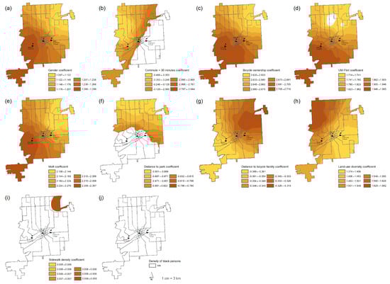
Figure 3.
Maps showing MTA bus routes and significant (±1.96) GWLR coefficients: gender (a), commute time > 30 min. (b), bicycle ownership (c), UM-Flint affiliation (d), MCC affiliation (e), distance to park (f), distance to bicycle facility (g), land-use diversity (h), sidewalk density (i), and density of black persons (j).
4. Discussion
Integrating bicycling and transit—including BoB—is part of an effective TDM toolkit, yet it is an often-overlooked travel consideration in practice and research within the U.S. [60,61]. This leaves us with an incomplete understanding of how to effectively promote this mode in cities and universities alike. The present study has added to the existing, albeit minimal, body of work examining BoB mode choice by showing how, and where, significant personal and neighborhood factors affect the probability of choosing BoB for the “first mile” portion of a university-based trip. Furthermore, the empirical analysis demonstrated that most respondents were generally uninterested in BoB; however, a small contingent residing close to the City’s CBD appeared willing to use this mode. The results of our discrete choice modeling strategy highlighted gender, commute time, and bicycle ownership were important personal factors; while park access, bicycle facility access, and land-use diversity, also influenced the probability of choosing this mode. The GWLR coefficient maps displayed the geographical impact of these factors; underscoring the importance of devising localized interventions to induce a mode shift towards BoB travel in a university environment.
Our first research objective (i) was to empirically and spatially describe the travel behaviors of the university sample, with a focus on BoB interest. The descriptive statistics showed that the majority of the sample utilized the automobile for non-university and university travel. We also saw that significant portions of the MCC and KU sample utilized transit and walking modes, respectively. One explanation for the elevated walking mode (max 34.4%) for the KU contingent is that 68.9% of the respondents reported commute times less than 10 min. We found that BoB interest was greatest among the UM-Flint and MCC sample—nearly 40% of the respondents stating “yes” to potentially using BoB. They also reported the longest commute times, high automobile accessibility, and reduced perceived access to bus stops. Thus, targeting groups from these two universities may have the largest impact on BoB mode choice. The ESDA (i.e., “hot-spot analysis”) showed where statistically significant clusters of university persons interested in BoB resided (see Figure 2c). We found that those living close to UM-Flint and the CBD were most interested in BoB, which is in part supported by past research showing interest in intermodal transportation is highest in urban areas [62]. Interestingly, despite slight interest in BoB from KU respondents, the university is close to groups of university constituents willing to use BoB. The result indicates that the attitudes towards BoB transportation are nuanced and may be attributed to university typology or local neighborhood conditions. Nonetheless, it highlights that context-sensitive planning and policy interventions are needed. Although some past research has shown that BoB mode shares are popular in the U.S. and a strong component of many university TDM strategies [8], we found the prospect of using this mode among our sample low, apart from a cluster near the City’s CBD.
The second objective (ii) of this research was to implement a discrete choice modeling framework—using two global models and one spatial model—to explain how much, and where, personal factors and neighborhood conditions affect BoB interest. Models 2 (GLR) and 3 (GWLR) were the strongest in terms of fit statistics; however, their explanatory power was modest (max R2 = 0.400). Nonetheless, we discovered several personal factors were associated with BoB interest. Males and bicycle owners favored BoB; the association was strongest in the City’s southwest neighborhoods. This finding finds support from previous works showing that males are more inclined to combine bicycling and transit [63] and tend to bicycle more than females [64]. Unsurprisingly, we found that bicycle ownership was also important when considering BoB modes; the finding builds on similar past works [65]. Combining bicycling and transit can be effective for medium or long commutes [66]; however, our results differ in that we found that the likelihood of using BoB diminished significantly for respondents living in the far northeast and southwest sections of the City, where commute times were greater than 30 min (>3 km from the City’s CBD). Due to the scarcity of bus routes in these areas (see Figure 1), and the importance of time for intermodal transport users [62], it isn’t unreasonable to infer that respondents may be opting to use the bicycle for their commute—because of its efficiency for long-distance travel [67], or the automobile. A logical intervention, therefore, would be to increase the level of transit service in periphery neighborhoods and examine bicycle facility access to ensure that these two modes can efficiently assimilate to promote BoB mode shares when traveling to the university.
Several neighborhood conditions were also found to affect probabilities of BoB mode choice. A noteworthy finding was the relationship between two accessibility indicators-parks and bicycle facilities—and BoB interest. The probability of using BoB modes decreased when respondents had limited access (i.e., increased distance) to parks: the northern half of the city exhibited the strongest relationship. Previous works highlighting the effect of park density on predicting intermodal transportation demonstrated a similar relationship [68]. Our results may also be an artifact of the known links between neighborhood quality, greenspace, and activity levels of the resident population [69]. In other words, the observed relationship found in this study may in part be linked to active residents self-selecting neighborhoods with elevated greenspace density, and perhaps inclined to choose active travel modes, such as BoB. Similar to past research speculating that bicycle network density has a minimal impact on bicycling rates to train stations [70], we discovered that overall neighborhood bikeability (i.e., BLOS) also showed no effect; rather, distance to a bicycle facility mattered. Therefore, a place-based strategy involving the installation of bicycle facilities (i.e., separated bicycle lanes, repair stations, and wayfinding signage) in areas that are safe and in high demand may elevate BoB interest for the “first-mile” of university travel. Our finding that land-use diversity had a positive impact on BoB interest resonates with previous research on bicycle transit integration [68]. We found that land-use diversity may persuade individuals to use this mode throughout the City, especially in neighborhoods northeast of the CBD (see Figure 3e). Areas in the southeast section showed a weaker relationship, highlighting that interventions may be needed there. To encourage BoB interest in these neighborhoods, it is suggested that the bus level of service be examined, and the MTA continues to work with the City to expand its bike-share network into these areas to ease bicycle–transit integration.
5. Conclusions
In this research, we examined how personal and neighborhood factors may influence the probability of choosing BoB mode choice among a university sample in Flint, Michigan. Our findings largely aligned with past research; however, we identified important associations not reported elsewhere. Despite these contributions, this study is not without limitations. First and foremost, this study was cross-sectional and very limited inferences about causality can be made. The sample size used in our study was small and may have inhibited reliable estimates, thereby reducing the generalizability of the research to other university populations. The sampling protocol enlisted a web survey, and did not solicit a random sample; therefore, the results herein should be interpreted with caution. The survey didn’t distinguish between faculty, staff, or students. Hence, we were unable to recommend specific interventions for any one university demographic. Additionally, the survey didn’t investigate perceived barriers or facilitators of BoB mode choice, nor did it ask about attitudes towards the local environment. Future work will aggregate such answers from a more expansive random sample. Other noteworthy inquiries will include attitudes towards the bicycle-bus boarding process, bicycle security during the trip, and conditions near egress points (i.e., the “last mile”), which has been shown to influence cycle-transit users [27]. Notwithstanding these limitations, the results from this research extend our knowledge of the influence of personal factors and neighborhood conditions on the willingness to use BoB for university travel purposes. In light of the ongoing motivation to create sustainable transportation systems in cities and university communities, it is hoped that the evidence provided in this study aids in developing more effective TDM policies to help meet this goal.
Author Contributions
Conceptualization, G.R.; data analysis, G.R.; writing—original draft preparation, G.R. and R.R.S.; writing—review and editing, R.R.S. Both authors have read and agreed to the published version of the manuscript.
Funding
This research received no external funding.
Institutional Review Board Statement
Not applicable.
Informed Consent Statement
Informed consent was obtained from all subjects involved in the study.
Data Availability Statement
The data presented in this study are available on request from the corresponding author. The data are not publicly available due to privacy concerns.
Acknowledgments
We would like to thank our MTA partners for their support and assistance with this study, Paul Mattern—Associate Transit Planner, and Leslie Phillips—Transit Clerk. We also appreciate Victoria Morckel’s many suggestions during manuscript preparation.
Conflicts of Interest
The authors declare no conflict of interest.
References
- Crane, P.; Kinzig, A. Nature in the metropolis. Science 2005, 308, 1225–1226. [Google Scholar] [CrossRef] [PubMed]
- UN. World Urbanization Prospects. The 2014 Revision; United Nations Department of Economics and Social Affairs, Population Division: New York, NY, USA, 2015; p. 41. [Google Scholar]
- Goletz, M.; Haustein, S.; Wolking, C.; L’Hostis, A. Intermodality in European metropolises: The current state of the art, and the results of an expert survey covering Berlin, Copenhagen, Hamburg and Paris. Transp. Policy 2020. [Google Scholar] [CrossRef]
- Shaker, R.R.; Altman, Y.; Deng, C.; Vaz, E.; Forsythe, K.W. Investigating urban heat island through spatial analysis of New York City streetscapes. J. Clean. Prod. 2019, 233, 972–992. [Google Scholar] [CrossRef]
- Rybarczyk, G.; Banerjee, S.; Starking-Szymanski, M.D.; Shaker, R.R. Travel and us: The impact of mode share on sentiment using geo-social media and GIS. J. Locat. Based Serv. 2018, 12, 40–62. [Google Scholar] [CrossRef]
- Sagaris, L.; Tiznado-Aitken, I.; Steiniger, S. Exploring the social and spatial potential of an intermodal approach to transport planning. Int. J. Sustain. Transp. 2017, 11, 721–736. [Google Scholar] [CrossRef]
- Shaker, R.R.; Rybarczyk, G.; Brown, C.; Papp, V.; Alkins, S. (Re) emphasizing Urban Infrastructure Resilience via Scoping Review and Content Analysis. Urban Sci. 2019, 3, 44. [Google Scholar] [CrossRef]
- Toor, W.; Havlick, S.W. Transportation & Sustainable Campus Communities: Issues, Examples, Solutions; Island Press: Washington, DC, USA, 2004. [Google Scholar]
- Newman, P.; Kenworthy, J.R. Sustainability and Cities: Overcoming Automobile Dependence; Island Press: Washington, DC, USA, 1999. [Google Scholar]
- Cheng, Y.-H.; Liu, K.-C. Evaluating bicycle-transit users’ perceptions of intermodal inconvenience. Transp. Res. Part A Policy Pract. 2012, 46, 1690–1706. [Google Scholar] [CrossRef]
- Yang, H.; Lu, X.; Cherry, C.; Liu, X.; Li, Y. Spatial variations in active mode trip volume at intersections: A local analysis utilizing geographically weighted regression. J. Transp. Geogr. 2017, 64, 184–194. [Google Scholar] [CrossRef]
- Pucher, J.; Buehler, R. Walking and cycling for healthy cities. Built Environ. 2010, 36, 391–414. [Google Scholar] [CrossRef]
- Gebhardt, L.; Krajzewicz, D.; Oostendorp, R. Intermodality—key to a more efficient urban transport system? In Proceedings of the 2017 Eceee Summer Study, Hyères, France, 29 May–3 June 2017; ECEEE Summer Study: Hyères, France, 2017; pp. 759–769. [Google Scholar]
- Martens, K. The bicycle as a feedering mode: Experiences from three European countries. Transp. Res. Part D Transp. Environ. 2004, 9, 281–294. [Google Scholar] [CrossRef]
- Krizek, K.J.; Stonebraker, E.W. Assessing options to enhance bicycle and transit integration. Transp. Res. Rec. 2011, 2217, 162–167. [Google Scholar] [CrossRef]
- Pucher, J.; Dill, J.; Handy, S. Infrastructure, programs, and policies to increase bicycling: An international review. Prev. Med. 2010, 50, 106–125. [Google Scholar] [CrossRef] [PubMed]
- Suzuki, H.; Cervero, R.; Iuchi, K. Transforming Cities with Transit: Transit and Land-Use Integration for Sustainable Urban Development; World Bank Publications: Washington, DC, USA, 2013. [Google Scholar]
- Maibach, E.; Steg, L.; Anable, J. Promoting physical activity and reducing climate change: Opportunities to replace short car trips with active transportation. Prev. Med. 2009, 49, 326–327. [Google Scholar] [CrossRef] [PubMed]
- Kager, R.; Harms, L. Synergies from Improved Cycling-Transit Integration: Towards an Integrated Urban Mobility System; Organisation for Economic Co-operation and Development (OECD): Paris, France, 2017. [Google Scholar]
- APTA. Public Transportation Fact Book; APTA: Washington, DC, USA, 2011. [Google Scholar]
- Flamm, B.; Rivasplata, C. Perceptions of Bicycle-Friendly Policy Impacts on Accessibility to Transit Services: The First and Last Mile Bridge; San Jose State University: San Jose, CA, USA, 2014; 100p. [Google Scholar]
- Hu, L.; Schneider, R.J. Shifts between automobile, bus, and bicycle commuting in an urban setting. J. Urban Plan. Dev. 2015, 141, 04014025. [Google Scholar] [CrossRef]
- Mees, P. Transport for Suburbia: Beyond the Automobile Age; Earthscan: London, UK, 2009. [Google Scholar]
- Hegger, R. Public transport and cycling: Living apart or together? Public Transp. Int. 2007, 56, 38–41. [Google Scholar]
- Pucher, J.; Buehler, R. Integrating bicycling and public transport in North America. J. Public Transp. 2009, 12, 5. [Google Scholar] [CrossRef]
- Ensor, M.; Slason, J. Forecasting the benefits from integrating cycling and public transport. In Proceedings of the Institution of Professional Engineers New Zealand (IPENZ) Transportation Conference, Auckland, New Zealand, 27–30 March 2011. [Google Scholar]
- Meenar, M.; Flamm, B.; Keenan, K. Mapping the Emotional Experience of Travel to Understand Cycle-Transit User Behavior. Sustainability 2019, 11, 4743. [Google Scholar] [CrossRef]
- Hagelin, C.A. Integrating bicycles and transit through bike-to-bus strategy. In Proceedings of the Transportation Research Board 86th Annual Meeting, Washington, DC, USA, 21–25 January 2007. [Google Scholar]
- Flamm, B.J. Determinants of bicycle-on-bus boardings: A case study of the Greater Cleveland RTA. J. Public Transp. 2013, 16, 4. [Google Scholar] [CrossRef]
- Bachand-Marleau, J.; Larsen, J.; El-Geneidy, A.M. Much-anticipated marriage of cycling and transit: How will it work? Transp. Res. Rec. 2011, 2247, 109–117. [Google Scholar] [CrossRef]
- Rybarczyk, G.; Gallagher, L. Measuring the potential for bicycling and walking at a metropolitan commuter university. J. Transp. Geogr. 2014, 39, 1–10. [Google Scholar] [CrossRef]
- UM-Flint Quick Facts-Student Body. Available online: https://www.umflint.edu/analysis/qf_student_body (accessed on 13 May 2020).
- Mott Community College. Demographic Profile by Term, 2019/2020; Mott Community College: Flint, MI, USA, 2018. [Google Scholar]
- Kettering University. Available online: https://www.usnews.com/best-colleges/kettering-university-2262 (accessed on 13 May 2020).
- Gold, R. UM-Flint Launches New Bike Share Program. M-Flint NOW, 23 December 2016. [Google Scholar]
- League of American Bicyclists. Bicycle Friendly University Current Awards. Available online: https://bikeleague.org/bfa/awards (accessed on 1 August 2020).
- Kettering University. Kettering University Launches Environmental Stewardship Focus Option for All Degrees. Available online: https://www.kettering.edu/news/kettering-university-launches-environmental-stewardship-focus-option-all-degrees (accessed on 7 August 2020).
- NBC25/Fox66 Mott Community College Holds Bicyle Safety Rodeo for Kids. Available online: https://nbc25news.com/news/local/mott-community-college-holds-bicyle-safety-rodeo-for-kids (accessed on 7 August 2020).
- Cervero, R.; Kockelman, K. Travel demand and the 3Ds: Density, diversity, and design. Transp. Res. Part D 1997, 2, 199–219. [Google Scholar] [CrossRef]
- Saelens, B.; Sallis, J.F.; Frank, L.D. Environmental Correlates of Walking and Cycling: Findings From the Transportation, Urban Design, and Planning Literatures. Ann. Behav. Med. 2003, 25, 80–91. [Google Scholar] [CrossRef] [PubMed]
- Ma, L.; Cao, J. How perceptions mediate the effects of the built environment on travel behavior? Transportation 2019, 46, 175–197. [Google Scholar] [CrossRef]
- Ramsey, K.; Bell, A. Smart Location Database, Version 2.0 User Guide, 2nd ed.; University of Southeastern Philippines: Davao City, Philippines, 2014; pp. 1–52. [Google Scholar]
- Rybarczyk, G.; Taylor, D.; Brines, S.; Wetzel, R. A Geospatial Analysis of Access to Ethnic Food Retailers in Two Michigan Cities: Investigating the Importance of Outlet Type within Active Travel Neighborhoods. Int. J. Environ. Res. Public Health 2020, 17, 166. [Google Scholar] [CrossRef] [PubMed]
- Li, L.; Du, Q.; Ren, F.; Ma, X. Assessing Spatial Accessibility to Hierarchical Urban Parks by Multi-Types of Travel Distance in Shenzhen, China. Int. J. Environ. Res. Public Health 2019, 16, 1038. [Google Scholar] [CrossRef]
- Landis, B.W.; Vattikuti, V.R.; Brannick, M.T. Real-Time Human Perceptions: Toward a Bicycle Level of Service. Transp. Res. Rec. 1997, 1578, 119–126. [Google Scholar] [CrossRef]
- Silverman, B.W. Density Estimation for Statistics and Data Analysis; CRC Press: Boca Raton, FL, USA, 1986; Volume 26. [Google Scholar]
- Anselin, L.; Li, X. Operational local join count statistics for cluster detection. J. Geogr. Syst. 2019, 21, 189–210. [Google Scholar] [CrossRef]
- Cervero, R.; Duncan, M. Walking, Bicycling, and Urban Landscapes: Evidence From the San Francisco Bay Area. Am. J. Public Health 2003, 93, 1478–1483. [Google Scholar] [CrossRef]
- Shaker, R.R.; Yakubov, A.D.; Nick, S.M.; Vennie-Vollrath, E.; Ehlinger, T.J.; Forsythe, K.W. Predicting aquatic invasion in Adirondack lakes: A spatial analysis of lake and landscape characteristics. Ecosphere 2017, 8, e01723. [Google Scholar] [CrossRef]
- Box, G.E.; Tidwell, P.W. Transformation of the independent variables. Technometrics 1962, 4, 531–550. [Google Scholar] [CrossRef]
- Hosmer, D.W., Jr.; Lemeshow, S.; Sturdivant, R.X. Applied Logistic Regression; Wiley: Hoboken, NJ, USA, 2013. [Google Scholar]
- Lee, S. Application of logistic regression model and its validation for landslide susceptibility mapping using GIS and remote sensing data. Int. J. Remote Sens. 2005, 26, 1477–1491. [Google Scholar] [CrossRef]
- Shaker, R.R. Examining sustainable landscape function across the Republic of Moldova. Habitat Int. 2016, 1–15. [Google Scholar] [CrossRef]
- Brunsdon, C.; Fotheringham, A.S.; Charlton, M.E. Geographically weighted regression: A method for exploring spatial nonstationarity. Geogr. Anal. 1996, 28, 281–298. [Google Scholar] [CrossRef]
- Nakaya, T. GWR4 User Manual. Available online: http://www.st-andrews.ac.uk/geoinformatics/wp-content/uploads/GWR4manual_201311.pdf (accessed on 4 November 2013).
- Fotheringham, A.S.; Crespo, R.; Yao, J. Geographical and Temporal Weighted Regression. Geogr. Anal. 2015, 47, 1–22. [Google Scholar] [CrossRef]
- Fotheringham, A.S.; Brunsdon, C.; Charlton, M. Geographically Weighted Regression: The Analysis of Spatially Varying Relationships; John Wiley & Sons: New York, NY, USA, 2002. [Google Scholar]
- Matthews, S.A.; Yang, T.-C. Mapping the results of local statistics: Using geographically weighted regression. Demogr. Res. 2012, 26, 151–166. [Google Scholar] [CrossRef]
- Rybarczyk, G. Toward a spatial understanding of active transportation potential among a university population. Int. J. Sustain. Transp. 2018, 12, 625–636. [Google Scholar] [CrossRef]
- Kager, R.; Bertolini, L.; Te Brömmelstroet, M. Characterisation of and reflections on the synergy of bicycles and public transport. Transp. Res. Part A Policy Pract. 2016, 85, 208–219. [Google Scholar] [CrossRef]
- Suraci, D. Bicycle and Transit Integration: A Practical Transit Agency Guide to Bicycle Integration and Equitable Mobility; APTA SUDS-UD-RP-009-18; American Public Transportation Association: Washington, DC, USA, 2018; pp. 1–53. [Google Scholar]
- Oostendorp, R.; Gebhardt, L. Combining means of transport as a users’ strategy to optimize traveling in an urban context: Empirical results on intermodal travel behavior from a survey in Berlin. J. Transp. Geogr. 2018, 71, 72–83. [Google Scholar] [CrossRef]
- Mohanty, S.; Blanchard, S. Complete transit: Evaluating walking and biking to transit using a mixed logit mode choice model. In Proceedings of the 95th Transportation Research Board Annual Meeting, Washington, DC, USA, 10–14 January 2016. [Google Scholar]
- Heinen, E.; Van Wee, B.; Maat, K. Commuting by bicycle: An overview of the literature. Transp. Rev. 2010, 30, 59–96. [Google Scholar] [CrossRef]
- Ji, Y.; Ma, X.; Yang, M.; Jin, Y.; Gao, L. Exploring spatially varying influences on metro-bikeshare transfer: A geographically weighted poisson regression approach. Sustainability 2018, 10, 1526. [Google Scholar] [CrossRef]
- Heinen, E.; Bohte, W. Multimodal Commuting to Work by Public Transport and Bicycle. Transp. Res. Rec. J. Transp. Res. Board 2014, 111–122. [Google Scholar] [CrossRef]
- Krizek, K.J.; Stonebraker, E.W. Bicycling and Transit. Transp. Res. Rec. J. Transp. Res. Board 2010, 2144, 161–167. [Google Scholar] [CrossRef]
- Zhao, P.; Li, S. Bicycle-metro integration in a growing city: The determinants of cycling as a transfer mode in metro station areas in Beijing. Transp. Res. Part A Policy Pract. 2017, 99, 46–60. [Google Scholar] [CrossRef]
- Maas, J.; Verheij, R.A.; Spreeuwenberg, P.; Groenewegen, P.P. Physical activity as a possible mechanism behind the relationship between green space and health: A multilevel analysis. BMC Public Health 2008, 8, 206. [Google Scholar] [CrossRef] [PubMed]
- Weliwitiya, H.; Rose, G.; Johnson, M. Bicycle train intermodality: Effects of demography, station characteristics and the built environment. J. Transp. Geogr. 2019, 74, 395–404. [Google Scholar] [CrossRef]
Publisher’s Note: MDPI stays neutral with regard to jurisdictional claims in published maps and institutional affiliations. |
© 2021 by the authors. Licensee MDPI, Basel, Switzerland. This article is an open access article distributed under the terms and conditions of the Creative Commons Attribution (CC BY) license (http://creativecommons.org/licenses/by/4.0/).