Article

Temporal-Spatial Structure and Influencing Factors of Urban Energy Efficiency in China’s Agglomeration Areas

School of Economics and Management, China University of Petroleum, Qingdao 266580, China
*
Author to whom correspondence should be addressed.
Sustainability 2021, 13(19), 10961; https://doi.org/10.3390/su131910961
Submission received: 11 September 2021 / Revised: 28 September 2021 / Accepted: 29 September 2021 / Published: 2 October 2021

Abstract

:
Energy efficiency has proved to be effective in mitigating greenhouse gas emissions and is significant to carbon neutrality targets. Urban agglomeration is the major engine of urbanization supporting economic growth. To optimizing the spatial exchange structure to improve regional energy efficiency by integrating the total factor energy efficiency model and social network analysis, this study constructs the spatial network of energy efficiency among cities within five major urban agglomerations in China for the period 2011–2018 and investigates their spatial association characteristics. The influencing factors of each spatial network structure are also explored by the quadratic assignment procedure method. The findings show that the spatial association of energy efficiency within each urban agglomeration presents a typical network structure, but with considerable disparity among urban agglomerations. Most cities in the Yangtze River Delta and Pearl River Delta are closely connected with each other, while the surrounding cities in the areas of Beijing-Tianjin-Hebei, Chengyu and the Middle Reaches of the Yangtze River highly depend on their corresponding central cities. The spatial adjacency and GDP per capita determine the urban spatial relationship of the energy efficiency within urban agglomerations. In addition, the spatial correlation of urban energy efficiency in the Beijing-Tianjin-Hebei, Chengyu and Middle Reaches of the Yangtze River areas is also affected by the differences in energy consumption, capital stock, number of labor force and pollutant emission. Some suggestions for improving urban energy efficiency are discussed.

1. Introduction

With economic development and intensive industrialization, humans have experienced a process of rapid urbanization during the past decades. Compared with only one-third of urban population in 1950, the world may roughly reverse the rural-urban population distribution by 2050 and about 70% of population will be settled in urban areas [1]. The positive effect of the sprawling of urban landscapes has been evidenced to be capable of increasing economic efficiency, such as sharping economic growth, rising incomes and increasing productivity [2]. Therefore, urban agglomeration, as an advanced spatial expressional form of integrated cities, can be the major engine of the urbanization for prosperous economic growth [3], and has encouraged widespread interests among the urban studies and geography communities [4]. Nevertheless, the development of urban agglomeration confronts challenges, especially on global climate change. Responsible for more than 70% of greenhouse gas emissions [5] and 67–76% of global energy use [6], urban areas have become the main battlefield in the fight against environmental and climate change. The process of urban agglomeration is proven to be able to alleviate greenhouse gas emissions [6]; however, a significant gap in achieving net zero emissions by the middle of the century still exists [7], and urban resilience for sustainable development is increasing [8]. With the further expansion of urban agglomerations, extra urban infrastructure and more energy consumption are inevitably required, which are major contributors to greenhouse gas emissions. How global economies can balance the development of urban agglomeration and the commitment of the greenhouse gas emissions is a sophisticated issue and should be thoroughly investigated.
In the past years, to meet climate targets, international scholars and organizations have reached a consensus on the matter that energy efficiency is the first fuel, and its improvement progress should be accelerated. In response, great efforts at various levels in academic communities have been made to evaluate energy efficiency, analyze the corresponding influencing factors, discuss the relationship between energy efficiency and economic growth and the spatial effects, etc. With respect to recent energy efficiency evaluation, Wang et al. [
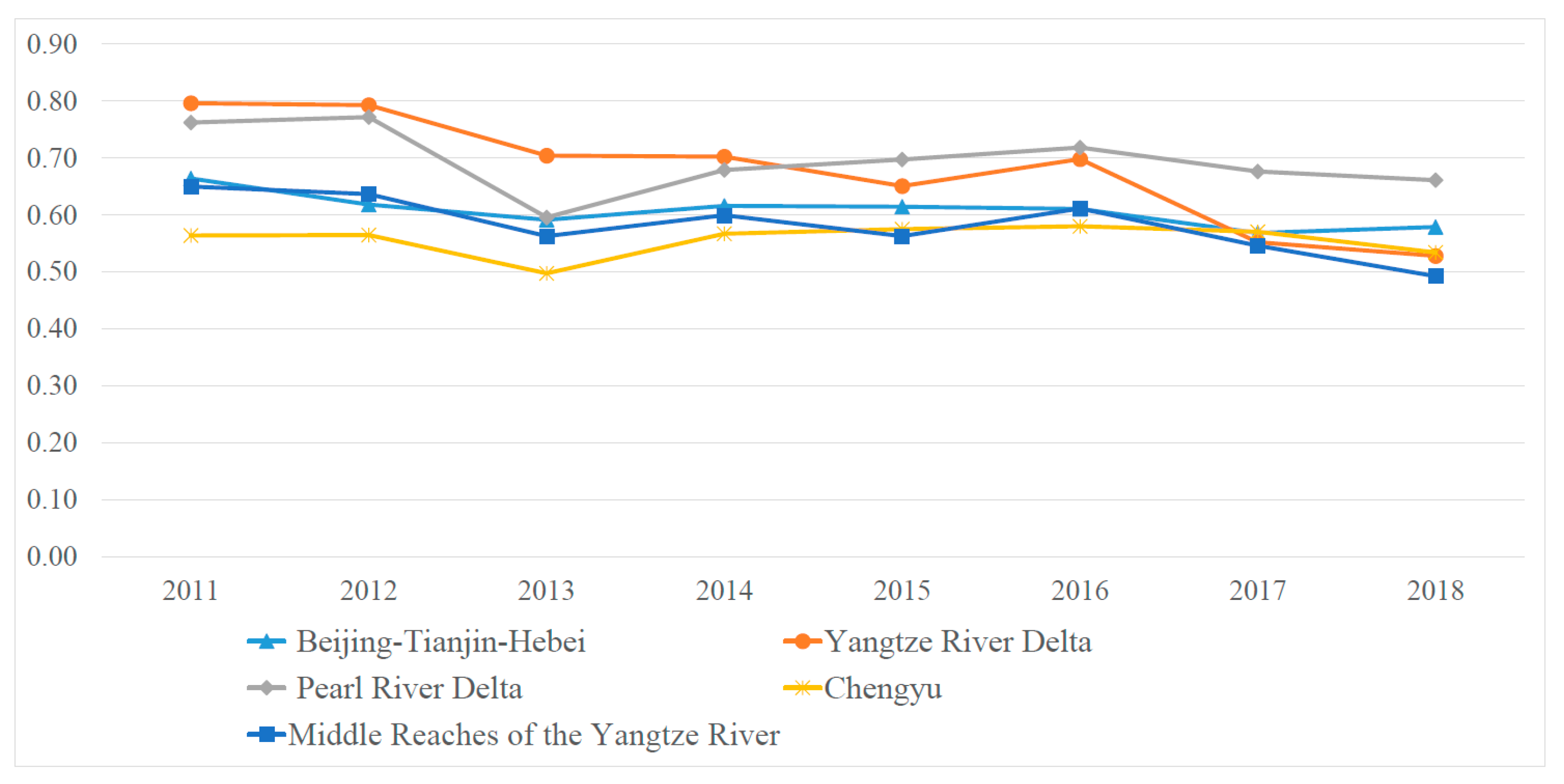
9] evaluated China’s regional energy efficiency performance by using the super efficiency data envelopment analysis and discussed regional disparity. During the past ten years, China’s regional energy efficiency is at a relatively low level, and the energy efficiency in the most developed region shows signs of downward trend. Li et al. [10] used a similar model to study the industrial total factor energy efficiency and concluded that there is still room for the improvement of energy efficiency in the industrial sector. Zhang et al. [11] considered the heterogenous impact on energy efficiency and conducted an empirical study on urban energy efficiency performance by combining the stochastic frontier analysis and the mean variance classification approach. They found that central cities with steady and relatively high energy efficiency can have significant impact on the energy efficiency improvement of their dependencies. Aldieri et al. [12] investigated energy efficiency for both developed and developing countries through a joint analysis of innovation, resilience, and adaptation via the conventional frontier model. In addition to the development of the frontier methods for the evaluation of energy efficiency, multicriteria decision-making methods are also explored in this field, see Bai et al. [13]. Another example is that a stochastic multicriteria acceptability analysis combining the preferences among energy trilemma was employed to measure national energy performance, see Song et al. [14]. In addition to the macro perspective, scholars also discuss the efficiency improvement of energy utilization from a micro technical perspective. For example, the contribution of energy-saving technologies in improving energy efficiency is valued by [15,16,17,18]. The promotion of EVs in the transportation sector provides a powerful way to improve overall energy efficiency.
Notably, the early energy efficiency evaluation studies mainly concentrated on how to maximize the positive effect of energy consumption on economic growth by adopting the single-factor energy efficiency index. However, this index takes energy consumption as the only input and fails to consider the possible substitution effect among different inputs such as energy, capital, or labor [19,20]. The single factor energy efficiency index ignores the undesired output in the production process [21]. Hence, Hu and Wang [22] first introduced the index of the total factor energy efficiency based on the data envelopment analysis by considering multiple input factors. Compared with the single factor energy efficiency index, the new index was more consistent with the real production process. Until now, the total factor energy efficiency has been a standard framework in assessing energy efficiency at different levels, e.g., [23,24,25,26,27,28,29].
To investigate how and what factors can influence the improvement of energy efficiency, many in-depth and detailed studies have been conducted. Meyer [30] reported the effectiveness of market forces to promote energy efficiency. Higher marketization can force market players to continuously accelerate the progress of energy efficiency with production optimization. The study by Birol and Keppler [31] emphasizes that the price of energy and new technologies are two important options to influence the changes in energy efficiency. The corresponding policies for these two options are suggested to be promoted simultaneously, rather than separately. The price factor is also proved by Steinbuks and Neuhoff [32] with an econometric analysis on five manufacturing industries. Sun et al.’s [33] research shows that the scale efficiency is the major contributor to the achievement of overall energy efficiency for resource-intensive cities, and a significant positive relationship exists between the urban population and urban energy efficiency. Recently, Liu et al. [34] provided some evidence to prove per capita GDP, industrial and transport structure, and fuel price all have a positive impact on the energy efficiency of the transport sector by integrating the Tobit censored model and the truncated model. In addition to these four factors, Liu and Lin [35] also confirmed that environmental protection can improve energy efficiency effectively. Besides, Li et al.’s [10] empirical study further is evidence that environmental regulation nonlinearly affects industrial energy efficiency with a U-shaped relationship, which may indicate that strong environmental regulation should be implemented for the improvement of energy efficiency in industries. From a spatial perspective, Cheng et al. [36] stated that different regions have significant differences of energy efficiency through the conditional convergence test. The studies conducted by Bai et al. [37] in the transportation industry supports this conclusion, and Zhang et al. [11] further found that the same influencing factors can have distinguished effects, especially considering the spatial and temporal dimensions. Du et al. [38] pioneered the discussion of the spatial impacts of urban agglomeration on urban energy efficiency based on a mono-index and panel data in China.
It is plausible to suppose that the spatial factors may significantly impact on the improvement of energy efficiency. Energy efficiency has a spatial spillover effect with technology diffusion efficiency in essence [39]. Regional energy efficiency can generate spatial spillover through an imitation and transmission mechanism [6,40,41]. Therefore, the promotion of energy efficiency may consider the urban area’s own use efficiency and others’ spillover effects simultaneously. However, as we noticed, most of the previous studies used “attribute data” to investigate the spatial differentiation of the energy efficiency. Peng et al. [42] criticized that “attribute data”-based studies can fail to reveal the structural characteristics of the spatial correlation. Structural characteristics often determine the performance of the “attribute data” and has more analytical value than “attribute data” [39]. In addition, traditional multiple linear regression and spatial econometric methods may limit the spatial correlation to the adjacent areas in geography [42]. Due to the improvement of infrastructure construction and the guidance of regional coordinated development policies, the production factors can exchange in a large spatial range. Traditional measurement methods may not thoroughly grasp the spatial structural correlation of energy efficiency among regions.
Hence, the network, which can contain multiple subjects and characterize structural features, has become a new method to study spatial relationships for improving the efficiency of policy implementation. For example, Bai et al. [37] discussed the spatial properties that provincial carbon emissions in the transportation section show in the form of the network structure. He et al. [43] empirically analyzed the network characteristics of carbon emissions in the electricity sector by integrating the social network analysis and gravity model and concluded China’s electricity sector shares a relatively stable overall network structure and are connected with each other closely. By an integrated analysis of network-oriented metrics, Gao et al. [44] investigated the embodied energy flow in a developing country under the foundation of handling the supply-demand security and climate change. Similarly, Lv et al. [45] investigated the embodied carbon transfer by joint analysis of multiregional input-output and social network analysis methods. Nevertheless, few studies are concerned about the spatial network structure of energy efficiency, especially in the areas of urban agglomeration. To the best of our knowledge, only Peng et al. [42] examined and demonstrated the spatial network structure and the corresponding characteristics of energy eco-efficiency in China’s Jiangsu Province.
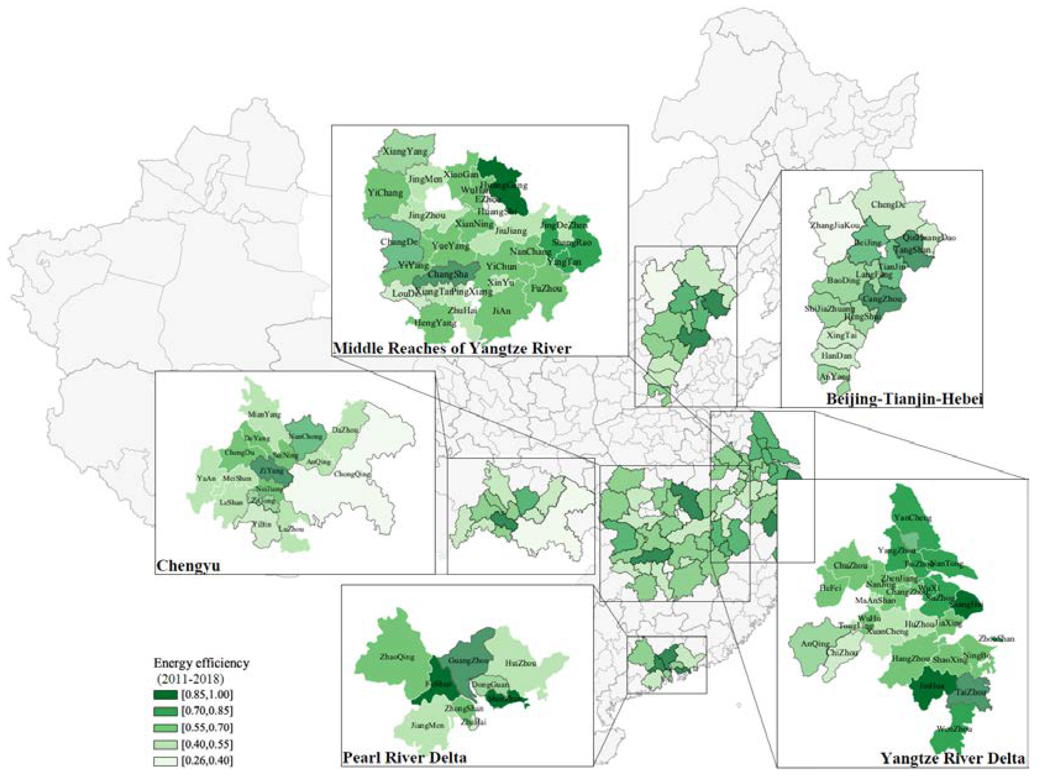
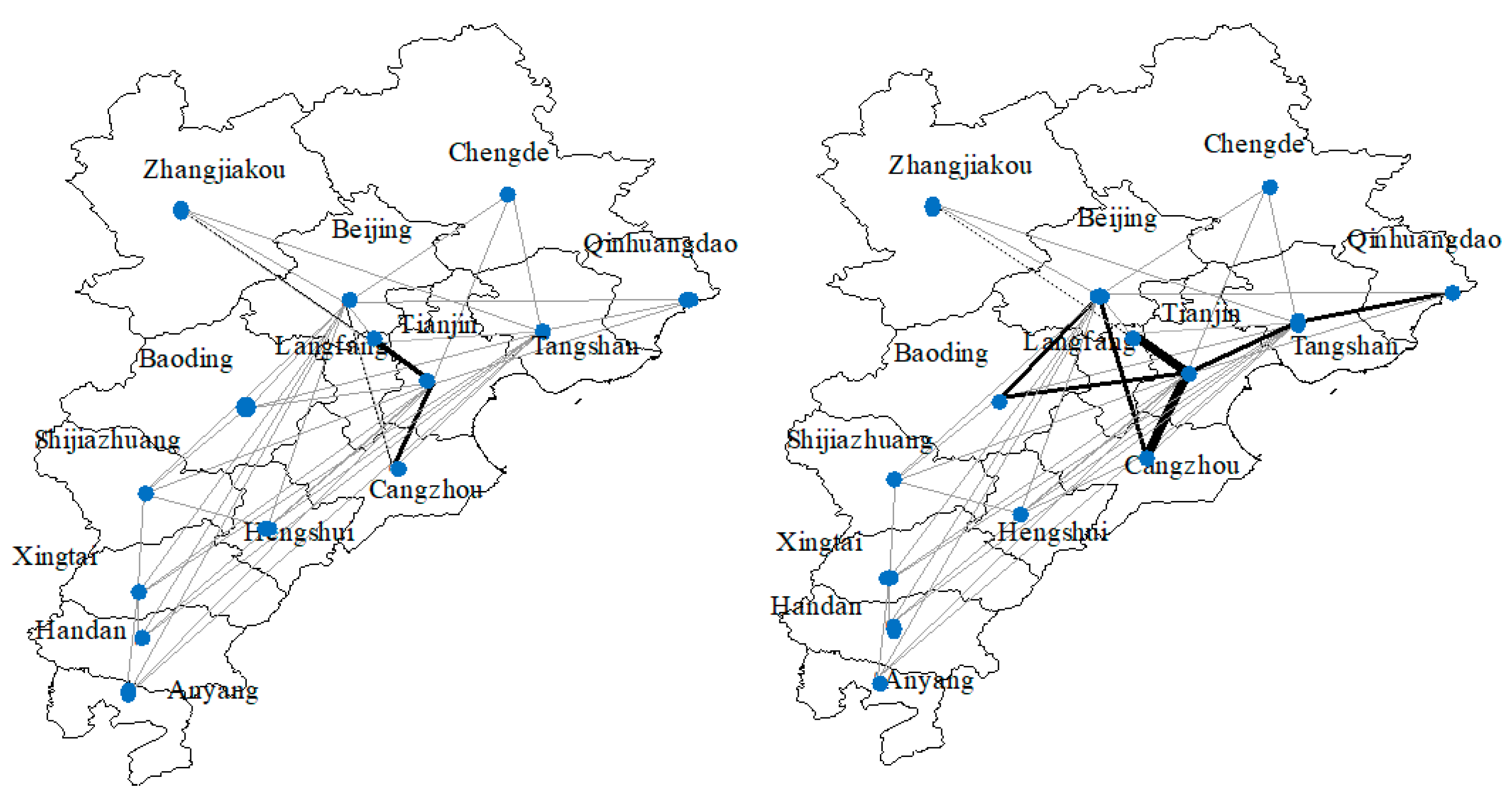
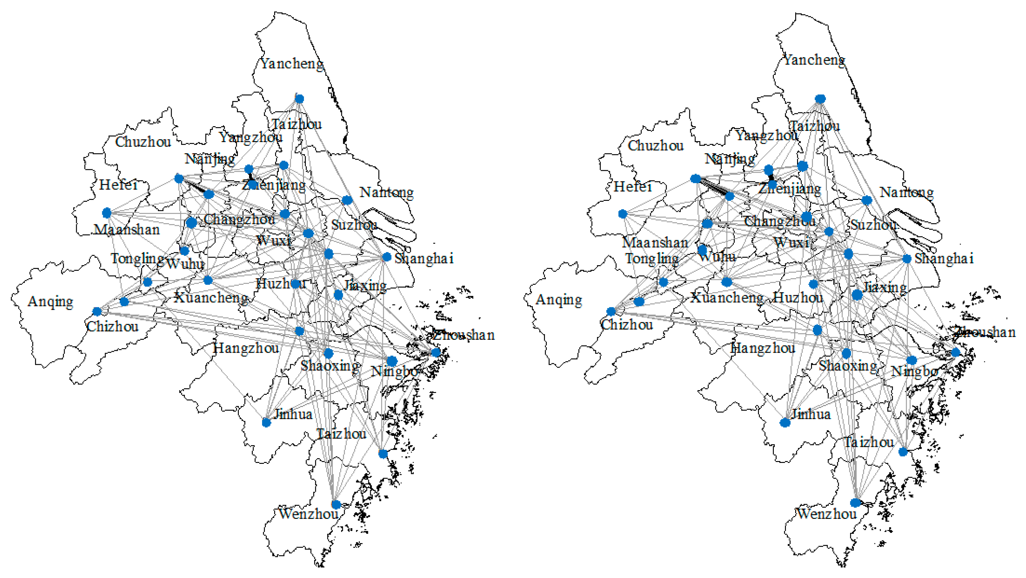
We address the gap by introducing the social network analysis method into the investigation of energy efficiency’s spatial structure characteristics in the China’s major urban agglomeration areas, i.e., Beijing-Tianjin-Hebei, the Yangtze River Delta and Pearl River Delta, Middle Reaches of the Yangtze River and Chengyu urban agglomerations. Currently, urban agglomeration is the major engine of the urbanization for supporting economic growth in China [3], emphasized in the latest Five-Year Plan of China for further coordinated regional development. Relatively, Beijing-Tianjin-Hebei, the Yangtze River Delta and Pearl River Delta are characterized by the fastest increase in population, and are marked the most urbanized and highly economic development in China. While the Middle Reaches of the Yangtze River and Chengyu urban agglomerations, as the emerging centers of the central and western regions, are also experiencing a rapid speed of development. In 2018, these major urban agglomerations accounted for 40% of the country’s total population and 53.7% of the country’s total GDP. As the largest developing country, China has committed to reach peak emissions before 2030 and become carbon neutral before 2060. In carbon neutrality, the prosperous development of urban agglomerations inevitably faces huge pressures. This study focuses on the spatial structure relationship of energy efficiency in the national urban agglomerations through constructing the association network of the urban total factor energy efficiency. Then the structural association relationship of the regional energy efficiency and the role of different cities in the corresponding energy efficiency network can be comprehensively investigated. We hope the empirical study can break the limits of the geographical location in the energy efficiency research communities and provide insights in balancing the development of urban agglomeration and the commitment of the carbon emissions. Moreover, the policy implications drawn from the investigation of the spatial interactive structure of cities in urban agglomeration areas may be more targeted to optimize the spatial structure among cities, and jointly improve the connected urban energy efficiency.
In general, the main contributions of our study are as follows. Firstly, we explore the possibility of employing a social network analysis in the investigation of energy efficiency’s spatial structure characteristics. The proposed framework by integrating the total factor energy efficiency model and social network analysis can be used to study the spatial differentiation of energy efficiency using structural data, comparatively. Secondly, our empirical study was conducted on China’s representative urban agglomeration areas. The findings can have an important impact on policy implications, especially to those spatial connected cities.
The remainder of this paper is organized as follows. Section 2 introduces the models employed to estimate the urban energy efficiency and to construct the corresponding spatial network structure of urban energy efficiency. A panel dataset is also introduced in this section. Based on the introduced models and dataset, Section 3 implements the empirical study and discusses the results. Section 4 summarizes this paper and proposes some suggestions. The symbols we introduced are listed in Nomenclature.

2. Methods and Data Description

2.1. Total Factor Energy Efficiency Estimation Model

The study takes each city as the decision-making unit (DMU) and defines E , N E , Y , B as energy inputs, non-energy inputs, and desirable outputs and undesirable outputs, respectively. The urban energy input is expressed by its energy consumption, which is calculated by converting different types of energy into standard coal (unit: 10,000 t of standard coal). The non-energy inputs include the capital stock and labor force (unit: 10,000 people), while the desirable outputs and undesirable outputs are expressed by the actual GDP (unit: CNY 100 million) and industrial sulfur dioxide emissions of each city (10,000 t), respectively. Under the total factor energy efficiency framework, the production technology can be described as T = { ( E , N E , Y , B ) : ( E , N E ) which can produce ( Y , B ) }. To reasonably simulate the joint production process of desirable and undesirable outputs, according to [19], the production technology set also needs to meet the weakly disposable and the null-jointness assumption. Following Zhou et al. [25] and Meng et al. [20], the non-radial directional distance function is expressed as:
D ( E , N E , Y , B ; g ) = s u p { w T β : ( ( E , N E , Y , B ) + g × d i a g ( β ) ) T } ,
where w = ( w E , w N E , w Y , w B ) , satisfying w E + w N E + w Y + w B = 1 , represents a standardized weight vector, which is related to the quantity of input and output. This vector allows decisionmakers to optimize input and output according to their importance. g = ( g E , g N E , g Y , g B ) is the directional vector, which specifies the direction of input and output change. β = ( β E , β N E , β Y , β B ) is a diagonal matrix, representing the adjustment amount of input decrease and output increase.
Then, under the scenario of energy conservation, emission reduction and economic growth, this study sets g = ( g E , g N E , g Y , g B ) = ( E , 0 , Y , B ) and w = ( w E , w N E , w Y , w B ) = ( 1 3 , 0 , 1 3 , 1 3 ) . Under constant returns to scale, following Zhou et al. [25], the production technology can be expressed as model (2).
D ( E , N E , Y , B ; g ) = m a x ( 1 3 β E + 1 3 β Y + 1 3 β B )
s . t .   n = 1 N Z n E n E E β E n = 1 N Z n N E n N E n = 1 N Z n Y n Y + Y β Y n = 1 N Z n B n B B β B Z n 0 ,   n = 1 ,   2 , ,   N 0 β E ,   β Y ,   β B < 1
Suppose D * is the optimal solution of model (2), the city’s total factor energy efficiency then can be expressed as E E = 1 D * . For easy implement of social network analysis, we normalize energy efficiency in (0, 100).

2.2. The Social Network Analysis Method

This study intends to deal with the spatial structures of energy efficiency in major urban agglomeration areas in China based on the social network analysis method. The spatial structure of energy efficiency can be captured by the spatial association network, which is explained as an aggregate of the energy efficiency relationships among cities within each urban agglomeration. Once the indicator measuring the relationship between cities satisfies a certain subjective threshold value, the corresponding relationship is significant, and a line can be drawn between cities with associated energy efficiency. Following this path, a network map of the spatial energy efficiency relationships in urban agglomeration can be created. Therefore, the underlying basis of the process is to represent complex and diverse relationship forms as certain network structures. The key to employing a social network analysis is the determination of the relationship among actors [39]. There are two main methods to determine the spatial correlation relationship. One is the gravity model, of which application examples can be found in [13,39,43,46]. The other is the Granger causality test based on the vector auto regression (VAR) method, see [42]. The gravity model cannot only describe the evolution trend of the spatial association network by using the cross-section data, but also consider the influence of distance factors on the association relationship, hence, gravity model, as shown by model (3), is adopted to construct the spatial correlation network of the energy efficiency among cities in urban agglomerations.
y i j = k m i m j d i j ,
where y i j represents the mutual correlation between energy efficiency of city i and j . m i and m j are the “mass” of i and j , respectively. d i j is the distance between two objects i and j . k is the empirical parameter. To employ the gravity model in our study, model (3) is modified as follows:
y i j = E E i E E i + E E j P i × E i × E E i 3 P j × E j × E E j 3 ( d i j e i e j ) 2 ,
where E E i ( j ) is the total factor energy efficiency of city i   ( j ) . The coefficient k is defined as k i j = ( E E i ) / ( E E i + E E j ) representing the contribution rate of the city i   in the energy efficiency connection between city i and j . P is the population and E is the city’s gross domestic product (GDP). Considering the influence of geographical and economic distance factors on the spatial correlation of the urban energy efficiency, 1 / ( e i e j ) is used to update the spatial distance in model (3). e is the per capita GDP in this study. Thus, d i j / ( e i e j ) represents the “economic geographical distance” between two cities. Then, y i j can be illustrated as the gravitational intensity of the energy efficiency between city i and j . According to model (4), the energy efficiency gravity matrix G i j between cities within urban agglomerations can be constructed as follows.
G i j = [ y 11 y 12 y 1 j y 21 y 22 y 2 j y i 1 y i 2 y i j ] ,
We first take the mean value of the gravity intensity of each row in the gravity matrix as the threshold value. If the gravity value y i j is greater than the threshold value of the corresponding row, then it is recorded as 1, which then indicates there is a significant correlation between the energy efficiency of cities i and j . Then we take cities i and j as nodes in the network map and draw a line between them. On the contrary, it is recorded as 0, indicating no significant correlation between the energy efficiency of city   i and j exists, and thus there is no line between them. After finishing the comparison, the spatial association network of the energy efficiency in China’s five urban agglomerations can be constructed.
Based on the constructed networks, we can identify specific influential cities and examine other important properties. For the purpose, overall and individual network characteristics are respectively measured by the following indexes. For investigating overall network characteristics, three indexes, that is network density, network connectedness and network hierarchy, are selected. Network density can capture the closeness of the constructed energy efficiency association network, which is expressed as:
D = L N × ( N 1 ) ,
where L is the number of network relationships, N × ( N 1 ) is the maximum possible number of network relationships. Greater values of the network density indicate energy efficiency has closer relationship between cities, and the network structure will have higher impact on the energy efficiency.
Network connectedness can capture the structure’s robustness and vulnerability of our constructed energy efficiency association network, which can be expressed as:
C = 1 V N × N 1 2 ,
where N is the number of cities in the network, and V is the number of unconnected point pairs. When C equals 1, we can assume that all cities within the urban agglomeration are in the individual network, and the constructed energy efficiency association network is robust. Otherwise, the network would be vulnerable.
Network hierarchy reflects the hierarchical structure of each city in the network. The network hierarchy H is expressed as:
H = 1 φ max ( φ ) ,
where φ is the number of paired cities that are symmetrically reachable in the constructed network, and max ( φ ) is the maximum possible number of symmetrically reachable cities. Greater values of the network hierarchy indicate the status difference among cities is more significant in the spatial energy efficiency correlation network, and more cities are subordinate and marginalized.
The characteristics of an individual network can be explored based on the concept of the centrality, which captures the importance of each city in the spatial energy efficiency association network. There are also three indicators can be employed, i.e., degree centrality, closeness centrality and betweenness centrality. Degree centrality reflects the virtual central position of each city in our spatial network. The cities with a higher degree centrality have more connections with others, that is, it is more in the center of the network, indicating it is more important in relation to other cities. The improvement of energy efficiency in other cities may substantially depend on the central cities. The calculation formula is:
D c = n N 1 ,
where n is the actual number of relationships associated with a city directly, and N is the maximum number of relationships that may be directly associated.
Closeness centrality is the inverse of the sum of average distances from one city to all other cities, and measures the mean distance from one city to other cities. It can be explained as the extent to which the energy efficiency of an individual city is not controlled by other cities. The higher the closeness centrality of a city is, the less likely it is to rely on other cities in the network to complete the connection, and the more direct connections it has with other cities. Cities with high closeness centrality can be regarded as central actors in the formation of network correlation. The calculation formula is as follows:
C d i = n j = 1 n d i j ,
where C d i is the closeness centrality of city i , d i j is the distance between city i and j .
Betweenness centrality measures the degree to which a city is on the path between other cities. For two cities in the spatial energy efficiency association network, there may be many shortest paths between them. We can calculate all the shortest paths between these two cities. If there are enough shortest paths passing through a city, it is considered that the betweenness centrality of this city is high, and the city can exert strong control over the interaction between other cities. This explanation implies that a city with higher betweenness centrality value can substantially influence other cities. The change in energy efficiency may be consistent between the city and its controlled other cities. The calculation formula is as follows:
C b i = 2 × j = 1 N k = 1 N b j k ( i ) N 2 3 N + 2 ,   j k i ,   and   j < k ,
b j k ( i ) = f j k ( i ) f j k is the ability of city i to control the association of j   and k . Where f j k is the number of shortcuts between two cities j and k , f j k ( i ) is the number of shortcuts through city i .
Notation
E Energy inputs
N E Non-energy inputs
Y Desirable outputs
B Undesirable outputs
w Standardized weight vector
g Directional vector
E E Total factor energy efficiency
e Per capita GDP
d i j Spherical distance between two cities
G i j Gravity matrix
D Network density index
C Network connectedness index
H Network hierarchy index
V The number of unreachable city pairs in the network
N The number of network nodes (cities)
φ The number of paired cities that are symmetrically reachable in the constructed network
D c Degree centrality index
C d i Closeness centrality index
C b i Betweenness centrality index
f j k The number of shortcuts between two cities j and k
f j k ( i ) The number of shortcuts which through city i .

2.3. Indicator and Data Source Description

Considering the study’s purpose and the availability of data, we collected the data from 94 cities in China’s five major urban agglomeration areas. In the energy efficiency calculation model, the energy input of a city is expressed by its energy consumption, which is calculated by converting different types of energy into standard coal. The non-energy inputs include capital stock and labor force, while the desirable outputs and undesirable outputs are expressed by the actual GDP and industrial sulfur dioxide emissions of each city, respectively. All data are from the China City Statistical Yearbook and the Statistical Bulletins. The conversion factors from physical unit to coal equivalent refers to the China Energy Statistical Yearbook. In the gravity model, the required data include the total factor energy efficiency of each city, population, GDP, the per capita GDP and the distance between cities. The distance between cities is represented by spherical distance, which is calculated by ArcGIS. The capital stock and GDP are deflated by 2011 = 100.

3. Results and Discussion

This section firstly uses model (2) to measure the energy efficiency of each city in China’s five urban agglomerations and analyzes the spatial and temporal distribution of energy efficiency of each urban agglomeration. Then, based on the modified gravity model (4), the spatial energy efficiency association network is constructed, and the network structure characteristics of spatial correlation are investigated. Finally, the factors that may affect the network structure are further discussed. The analytical process is shown in Figure 1.

3.1. Spatial-Temporal Distribution Analysis of Energy Efficiency

Based on model (2), the total factor energy efficiency of 94 cities within five urban agglomeration areas is calculated for the period of 2011 to 2018. The changes in average energy efficiency of 94 cities within five urban agglomeration areas are illustrated in Figure 2, showing that the overall trend is downward despite a certain degree of fluctuations. The urban energy efficiency performance of the Yangtze River Delta region is competitive in 2014 and before, however, with the largest decrease from 0.80 in 2011 to 0.53 in 2018. The urban energy efficiency performance of the Pearl River Delta region is generally better than that of cities in other urban agglomeration areas, although its energy efficiency declined significantly in 2013. The urban energy efficiency performance in the remaining urban agglomeration areas is relatively stable with slight a decrease for the period. Relatively, the urban average energy efficiency within the different urban agglomerations in different years shows diversity and disparity. Cities in relative mature urban agglomerations, such as the Yangtze River Delta region and the Pearl River Delta region, may have a higher energy efficiency performance, while, in emerging urban agglomerations, such as the Middle Reaches of the Yangtze River region and Chengyu region, are accompanied by a lower performance.
To further investigate the spatial and temporal distribution of urban energy efficiency in different urban agglomerations, we compared the average energy efficiency in each urban agglomeration for the period of 2011 to 2018, as illustrated in Figure 3. In the Beijing-Tianjin-Hebei region, Beijing, Tianjin, Tangshan and Cangzhou have a relatively higher energy efficiency. While peripheral cities, such as Handan, Qinhuangdao, Xingtai and Zhangjiakou, have the lowest energy efficiency. The energy efficiency distribution of the Yangtze River Delta urban agglomeration shows the spatial characteristics of “polarization”, the energy efficiency of the central cities is obviously lower than that of northern and southern cities in this area; while the energy efficiency in Pearl River Delta has the characteristic of “centralization”. The energy efficiency of the central region exceeds the average level of the studied urban agglomerations. For the remaining urban agglomerations, due to the relatively weak level of economic development, their coordinated development of energy, economy and environment are lower than these two urban agglomerations. Moreover, the energy efficiency in all urban agglomerations shows spatial imbalance. In the Chengyu urban agglomeration, Ziyang has the highest energy efficiency which reaches 1, compared with only 0.3407 for Chongqing. The energy efficiency of the spatial distribution in the Middle Reaches of the Yangtze River shows no obvious clustering during the whole sample period.

3.2. Spatial Association Analysis

3.2.1. Overall Network Structure and Evolution Trend

The spatial energy efficiency association networks were constructed using the modified gravity model, as illustrated in Figure 4, Figure 5, Figure 6, Figure 7, Figure 8. Based on the overall network characteristic indexes, the network correlation in each sample urban agglomeration equals 1 from 2011 to 2018, which indicates that all cities are in their spatial association network, and the energy efficiency within each urban agglomeration has a significant spatial correlation relationship.
Figure 9 depicts the evolution trend of network density. It can be seen from Figure 4 that the network density of all urban agglomerations does not fluctuate significantly from 2011 to 2018. This indicates that the development of urban agglomerations does not enhance the spatial correlation and stability of energy efficiency among cities. The numerical results of the network density are not high within the five urban agglomerations. For example, the Pearl River Delta area has the highest network density, but its average actual relationship number is only 23, and the total number of its maximum possible relationship equals 72. The linkages between urban energy efficiency still have the enhanced space significance.
Figure 10 shows the network hierarchy of five urban agglomerations. As we can see from Figure 10, there are two cases: except the Pearl River Delta and the Yangtze River Delta, the network hierarchy of other urban agglomerations presents an upward trend during 2016–2018. The difference of position between cities is increasing, and more cities are in the subordinate or marginalized position in the spatial correlation network of the Beijing-Tianjin-Hebei, Chengyu and Middle Reaches of the Yangtze River areas. The presented network structure may be related to the hierarchical gap within the urban agglomeration itself. Restricted by the development levels, non-central cities have a limited ability to receive the radiation from the core cities, which makes it increasingly difficult for them to share the resources of the central cities. Combining Figure 5 with Figure 7 and Figure 8, for the Yangtze River Delta and the Pearl River Delta, their spatial correlation distribution is relatively balanced, there are correlations in almost all cities. For the network structures of other three urban agglomerations, it can be seen that more cities spread outward along the “supporting points”, while there is almost no correlation between other cities.

3.2.2. Centrality Analysis

To identify the position and the role of cities in the network, the index of degree centrality, closeness centrality and betweenness centrality in each urban agglomeration are analyzed. Table 1, Table 2, Table 3, Table 4, Table 5 show the centrality results of each urban agglomeration in 2018.
As shown in Table 1, the mean values of the three centralities in Beijing-Tianjin-Hebei are 42.857, 65.532, and 6.502, respectively. Among them, the cities with a higher degree centrality, closeness centrality and betweenness centrality were Beijing, Tianjin, and Tangshan. That is, the cities present the feature of the largest number of correlation relationships, “closest” to other cities, and lead the communication within the urban agglomeration. Restricted by economic development level and geographical location, Handan, Anyang, and Zhangjiakou have less correlation with others and are positioned as the periphery of the network.
As shown in Table 2, the city centrality in the Yangtze River Delta is relatively balanced. Compared with other urban agglomerations, the results in Yangtze River Delta have lower standard deviations. Specifically, the centrality values of Wuxi, Suzhou, and Changzhou are significantly higher than those of other cities, which means Wuxi, Suzhou, and Changzhou locate in the core area of the network, and they have strong agglomeration and radiation functions. For other sub-central cities, they also have higher central values. The mean values of these three centrality values in the Yangtze River Delta urban agglomeration are 37.322, 59.700, and 5.145, respectively. Regarding the degree centrality and closeness centrality, 12 cities go beyond the average level, and 10 cities go beyond the mean values of betweenness centrality. Moreover, it is worth noting that Shanghai does not occupy a dominant position in the network despite a high level of energy efficiency. Particularly, its betweenness centrality is significantly lower than the average, which may be related to its geographical location. From an overall viewpoint, cities that play a larger “intermediary” role, are most located in the central region of the Yangtze River Delta urban agglomeration. Tongling, Chizhou, and Nantong have the lowest centrality value. Hence there may be a certain degree of difficulty for them to insert an influence on the correlation relationship in the network.
In the Pearl River Delta area, the centrality values of Shenzhen and Guangzhou are higher than those of other cities, as shown in Table 3. In the network, they have the most direct connection and the shortest element communication distance with other cities. It is worth noting that although the energy efficiency level of Jiangmen and Dongguan is low, the degree centrality and closeness centrality of Jiangmen are lower only than that of Shenzhen and Guangzhou, which may have an impact on the energy efficiency of other cities in the network. This is a problem worthy of our attention, because after long-term development, this feature key city with low efficiency, may cause further widening of the energy efficiency gap within the Pearl River Delta urban agglomeration.
In the network of the Chengyu area, Table 4 shows that the cities with higher centrality are mainly concentrated in the main axis of the Chengdu-Chongqing development, such as Chengdu, Chongqing, Zigong, Nanchong, and Deyang. Chengdu is in the absolute center of the network because of its good economic foundation and technical level. However, as another important development center in this area, Chongqing has a low communication efficiency with other cities in the network, its degree centrality and closeness centrality are relatively low. In addition, in the spatial correlation network of energy efficiency in the Chengyu area, two-fifths of the cities, such as Mianyang, Meishan, Yibin, Dazhou, Yaan, and Ziyang, have a betweenness centrality of 0. This shows that in the spatial correlation network of the Chengyu urban agglomeration, there is an obvious gap in the participation degree of each city.
As depicted in Table 5, there exists a huge difference in the degree centrality in the Middle Reaches of the Yangtze River urban agglomeration. The core position of Changsha is obvious. This characteristic is similar to the network structure dominated by Chengdu in Chengyu Urban Agglomeration. In addition, about 70% of the cities’ values are below the mean centrality. Therefore, there are great communication obstacles and marginalization risks in the spatial correlation network of energy efficiency.

3.3. Influencing Factor Analysis

According to the above empirical analysis results, the energy efficiency spatial correlation network structure of China’s five major urban agglomerations presents its own characteristics. This part further explores the factors influencing the differences in the network structure characteristics of urban agglomerations and reveals the formation mechanism of the spatial association network. Since relational data, in which variables are not independent of each other, is studied based on a social network analysis in this study, the quadratic assignment procedure (QAP) method is used for the correlation and regression analysis following [43,45]. The QAP model is constructed as follows:
T = f ( D , C , E , K , L , B ) ,
where T refers to the binary network matrix of spatial association of urban agglomerations. D is the geographical distance association matrix. If two cities are adjacent, the corresponding element value in D is 1, otherwise, 0. C is the difference matrix of per capita GDP, which is used to represent the gap of urban economic development. E ,   K ,   L and B are the difference matrices of input-output variables respectively. E is the difference matrix of energy consumption. K is the capital stock difference matrix. L is the labor force difference matrix. B is pollutant discharge difference matrix. Except for D , other explanatory variables are composed of the absolute value difference of each city in 2018. All difference matrices are also normalized to eliminate the dimensionality effect.
In the QAP correlation analysis, this study sets the number of random permutations as 5000 times. The correlation results of the spatial association network in urban agglomerations and influencing factors are shown in Table 6. The influence of above factors on the spatial correlation network structure in different urban agglomerations is heterogeneous. For the Beijing-Tianjin-Hebei and the Middle Reaches of the Yangtze River urban agglomerations, the six explanatory variables are all important factors affecting the formation of their spatial association network. For the Yangtze River Delta and Pearl River Delta urban agglomerations, which have higher energy efficiency levels, they also have similarities in the formation mechanism of their spatial association network: spatial adjacency (D) and difference of per capita GDP (C) are the key factors affecting the formation of the spatial association network, while other factors have no significant influence.
QAP regression results of each urban agglomeration are shown in Table 7. It can be seen that at the significance level of 1%, D and C have a positive effect on the spatial correlation effect of energy efficiency in each urban agglomeration. This indicates that the spatial correlation of energy efficiency is more likely to occur between geographically adjacent regions, and the larger the gap of economic development level, the more attraction provided to the cross-regional flow of factors, which is conducive to the formation of the spatial association network. At the significance level of 5% and 10%, E shows the opposite effect on the spatial correlation of the Beijing-Tianjin-Hebei and Chengyu urban agglomeration, respectively: with the expansion of energy consumption differences, the spatial correlation of energy efficiency is more likely to occur in the Beijing-Tianjin-Hebei urban agglomeration, but it is not conducive to the formation of the association network for the Chengyu urban agglomeration. In addition, for the influencing factors K and B, except for the spatial correlation of Chengyu urban agglomeration, the test results of K for other urban agglomerations are not significant. B only showed a significant negative correlation for the spatial correlation of the Middle Reaches of the Yangtze River urban agglomerations. This indicates that Chengyu and the Middle reaches of the Yangtze River, which have a relatively low degree of integration, still have some problems in the effective integration of resources, capital, and technology.

4. Conclusions

In this study, five spatial correlation networks of urban energy efficiency in five Chinese urban agglomerations were constructed. Then, technologies of social network analysis and QAP were used to investigate the structural characteristics and influencing factors of the energy efficiency spatial correlation network, respectively. Based on the empirical analysis, the main conclusions were drawn. First, the energy efficiency shows obvious differences among five urban agglomerations. Second, the spatial correlation of energy efficiency in five urban agglomerations all present a typical network structure, but with great differences. The spatial association network structure in the Beijing-Tianjin-Hebei, Chengyu and Middle Reaches of the Yangtze River areas shows the characteristics of “polarization”. While the spatial structures in Yangtze River Delta and Pearl River Delta present a more balanced feature. Finally, the results from the QAP analysis show that spatial adjacency and per capita GDP difference are the main factors affecting the spatial correlation of urban agglomerations. In addition, the spatial correlation of the urban energy efficiency in the Beijing-Tianjin-Hebei, Chengyu and Middle Reaches of the Yangtze River areas is also affected by the differences in energy consumption, capital stock, number of labor force and pollutant emission to varying degrees.
The empirical study provides a reference for cities to choose partners and formulate trans-regional policies to improve regional energy efficiency comprehensively. Additionally, by optimizing the spatial correlation structure, cooperation within the urban agglomeration can be strengthened, which also contributes to the diffusion of energy conservation and emission reduction effects. The role of cities in the spatial correlation network should be fully considered. Since cities with high central values are the key drivers of network connection, policies can be implemented according to the role of each city, so as to improve the efficiency of energy policy implementation. Finally, based on the analysis of the factors affecting the spatial correlation network of energy efficiency, policymakers may exert the instruments of government macro-control and market mechanisms to improve the spatial correlation of energy efficiency.

Author Contributions

Conceptualization, methodology, validation, and writing—review and editing, L.Z. and L.F.; software, resources, data curation, and writing—original draft preparation, L.Z. and Y.Z.; funding acquisition, L.F. All authors have read and agreed to the published version of the manuscript.

Funding

This research was funded by the National Social Science Fund of China, grant number 17BGL251.

Institutional Review Board Statement

Not applicable.

Informed Consent Statement

Not applicable.

Data Availability Statement

The data that support the plots within this paper and other findings of this study are available from the corresponding author upon reasonable request.

Conflicts of Interest

The authors declare no conflict of interest.

Nomenclature

GHGGreenhouse gas emissions
VARVector auto regression
GDPGross domestic product
TFEETotal factor energy efficiency
DEAData envelopment analysis
DMUDecision-making unit
SNASocial network analysis
UAUrban agglomeration area
QAPQuadratic assignment procedure method

References

  1. United Nations; Department of Economic and Social Affairs; Population Division. World Urbanization Prospects: The 2018 Revision (ST/ESA/SER.A/420); United Nations: New York, NY, USA, 2019. [Google Scholar]
  2. Spence, M.; Annez, P.C.; Buckley, R.M. Urbanization and Growth; World Bank Publications: Washington, DC, USA, 2008. [Google Scholar]
  3. Tang, L.; Li, K. A comparative analysis on energy-saving and emissions-reduction performance of three urban agglomerations in China. J. Clean. Prod. 2019, 220, 953–964. [Google Scholar] [CrossRef]
  4. Fang, C.; Yu, D. Urban agglomeration: An evolving concept of an emerging phenomenon. Landsc. Urban Plan. 2017, 162, 126–136. [Google Scholar] [CrossRef]
  5. IEA. World Energy Outlook 2012; IEA: Paris, France, 2012; Available online: https://www.iea.org/reports/world-energy-outlook-2012 (accessed on 8 June 2021).
  6. Yu, X.; Wu, Z.; Zheng, H.; Li, M.; Tan, T.; Yu, X.; Wu, Z.; Zheng, H.; Li, M.; Tan, T. How urban agglomeration improve the emission efficiency? A spatial econometric analysis of the Yangtze River Delta urban agglomeration in China. J. Environ. Manag. 2020, 260, 110061. [Google Scholar] [CrossRef]
  7. United Nations Environment Programme (UNEP). Emissions Gap Report 2020; UNEP: Nairobi, Kenya, 2020. [Google Scholar]
  8. Nazarnia, H.; Nazarnia, M.; Sarmasti, H.; Wills, W.O. A Systematic Review of Civil and Environmental Infrastructures for Coastal Adaptation to Sea Level Rise. Civ. Eng. J. 2020, 6, 1375–1399. [Google Scholar] [CrossRef]
  9. Wang, R.; Wang, Q.; Yao, S. Evaluation and difference analysis of regional energy efficiency in China under the carbon neutrality targets: Insights from DEA and Theil models. J. Environ. Manag. 2021, 293, 112958. [Google Scholar] [CrossRef]
  10. Li, Y.; Xu, X.; Zheng, Y. An Empirical Study of Environmental Regulation Impact on China’s Industrial Total Factor Energy Efficiency: Based on the Data of 30 Provinces from 2003 to 2016. Manag. Rev. 2019, 31, 40. [Google Scholar]
  11. Zhang, H.; Fan, L.; Zhou, P. Handling heterogeneity in frontier modeling of city-level energy efficiency: The case of China. Appl. Energy 2020, 279, 115846. [Google Scholar] [CrossRef]
  12. Aldieri, L.; Gatto, A.; Vinci, C.P. Evaluation of energy resilience and adaptation policies: An energy efficiency analysis. Energy Policy 2021, 157, 112505. [Google Scholar] [CrossRef]
  13. Bai, Y.; Zhou, P.; Tian, L.; Meng, F. Desirable Strategic Petroleum Reserves Policies in Response to Supply Uncertainty: A Stochastic Analysis. Appl. Energy 2016, 162, 1523–1529. [Google Scholar] [CrossRef]
  14. Song, L.; Fu, Y.; Zhou, P.; Lai, K.K. Measuring National Energy Performance via Energy Trilemma Index: A Stochastic Multicriteria Acceptability Analysis. Energy Econ. 2017, 66, 313–319. [Google Scholar] [CrossRef]
  15. Ding, X.; Wang, Z.; Zhang, L. Hybrid Control-Based Acceleration Slip Regulation for Four-Wheel-Independent-Actuated Electric Vehicles. IEEE Trans. Transp. Electrif. 2021, 7, 1976–1989. [Google Scholar] [CrossRef]
  16. Gorbunova, A.D.; Anisimov, I.A. Assessment of the Use of Renewable Energy Sources for the Charging Infrastructure of Electric Vehicles. Emerg. Sci. J. 2020, 4, 539–550. [Google Scholar] [CrossRef]
  17. Zhang, L.; Wang, Y.; Wang, Z. Robust Lateral Motion Control for In-Wheel-Motor-Drive Electric Vehicles with Network Induced Delays. IEEE Trans. Veh. Technol. 2019, 68, 10585–10593. [Google Scholar] [CrossRef]
  18. Zhang, L.; Wang, Z.; Ding, X.; Li, S.; Wang, Z. Fault-Tolerant Control for Intelligent Electrified Vehicles Against Front Wheel Steering Angle Sensor Faults During Trajectory Tracking. IEEE Access 2021, 9, 65174–65186. [Google Scholar] [CrossRef]
  19. Wang, H.; Zhou, P.; Zhou, D. Scenario-based energy efficiency and productivity in China: A non-radial directional distance function analysis. Energy Econ. 2013, 40, 795–803. [Google Scholar] [CrossRef]
  20. Meng, F.; Fan, L.; Zhou, P.; Zhou, D. Measuring environmental performance in China’s industrial sectors with non-radial DEA. Math. Comput. Model. 2013, 58, 1047–1056. [Google Scholar] [CrossRef]
  21. Wang, K.; Wei, Y.-M.; Zhang, X. A comparative analysis of China’s regional energy and emission performance: Which is the better way to deal with undesirable outputs? Energy Policy 2012, 46, 574–584. [Google Scholar] [CrossRef]
  22. Hu, J.-L.; Wang, S.-C. Total-factor energy efficiency of regions in China. Energy Policy 2006, 34, 3206–3217. [Google Scholar] [CrossRef]
  23. Mandal, S.K. Do undesirable output and environmental regulation matter in energy efficiency analysis? Evidence from Indian Cement Industry. Energy Policy 2010, 38, 6076–6083. [Google Scholar] [CrossRef]
  24. Färe, R.; Grosskopf, S. Directional distance functions and slacks-based measures of efficiency. Eur. J. Oper. Res. 2010, 200, 320–322. [Google Scholar] [CrossRef]
  25. Zhou, P.; Ang, B.; Wang, H. Energy and CO2 emission performance in electricity generation: A non-radial directional distance function approach. Eur. J. Oper. Res. 2012, 221, 625–635. [Google Scholar] [CrossRef]
  26. Wu, F.; Fan, L.; Zhou, P.; Zhou, D. Industrial energy efficiency with CO2 emissions in China: A nonparametric analysis. Energy Policy 2012, 49, 164–172. [Google Scholar] [CrossRef]
  27. Wu, F.; Zhou, P.; Zhou, D. Does Congestion Affect Total-Factor Energy Efficiency? A Theoretical Study. Energy Procedia 2014, 61, 294–298. [Google Scholar] [CrossRef] [Green Version]
  28. Wang, Q.; Su, B.; Sun, J.; Zhou, P.; Zhou, D. Measurement and decomposition of energy-saving and emissions reduction performance in Chinese cities. Appl. Energy 2015, 151, 85–92. [Google Scholar] [CrossRef]
  29. Zhang, N.; Zhou, M. The inequality of city-level energy efficiency for China. J. Environ. Manag. 2020, 255, 109843. [Google Scholar] [CrossRef]
  30. Meyers, S. Improving Energy Efficiency: Strategies for Supporting Sustained Market Evolution in Developing and Transitioning Countries; Lawrence Berkeley National Laboratory: Berkeley, CA, USA, 1998. [Google Scholar]
  31. Birol, F.; Keppler, J.H. Prices, technology development and the rebound effect. Energy Policy 2000, 28, 457–469. [Google Scholar] [CrossRef]
  32. Steinbuks, J.; Neuhoff, K. Assessing energy price induced improvements in efficiency of capital in OECD manufacturing industries. J. Environ. Econ. Manag. 2014, 68, 340–356. [Google Scholar] [CrossRef] [Green Version]
  33. Sun, W.; Li, Y.; Wang, D.; Fan, J. The Efficiencies and Their Changes of China’s Resources-Based Cities Employing DEA and Malmquist Index Models. J. Geogr. Sci. 2012, 22, 509–520. [Google Scholar] [CrossRef]
  34. Liu, H.; Li, J.; Long, H.; Li, Z.; Le, C. Promoting energy and environmental efficiency within a positive feedback loop: Insights from global value chain. Energy Policy 2018, 121, 175–184. [Google Scholar] [CrossRef]
  35. Liu, W.; Lin, B. Analysis of energy efficiency and its influencing factors in China’s transport sector. J. Clean. Prod. 2018, 170, 674–682. [Google Scholar] [CrossRef]
  36. Cheng, Z.; Liu, J.; Li, L.; Gu, X. Research on meta-frontier total-factor energy efficiency and its spatial convergence in Chinese provinces. Energy Econ. 2020, 86, 104702. [Google Scholar] [CrossRef]
  37. Bai, C.; Zhou, L.; Xia, M.; Feng, C. Analysis of the spatial association network structure of China’s transportation carbon emissions and its driving factors. J. Environ. Manag. 2020, 253, 109765. [Google Scholar] [CrossRef]
  38. Du, J.; Zhao, M.; Zeng, M.; Han, K.; Sun, H. Spatial Effects of Urban Agglomeration on Energy Efficiency: Evidence from China. Sustainability 2020, 12, 3338. [Google Scholar] [CrossRef] [Green Version]
  39. Liu, H.; Liu, C.; Sun, Y. Spatial Correlation Network Structure of Energy Consumption and Its Effect in China. China Ind. Econ. 2015, 5, 83–95. (In Chinese) [Google Scholar]
  40. Chen, J.; Xu, C.; Song, M.; Liu, X. Driving factors of China’s energy productivity and its spatial character: Evidence from 248 cities. Ecol. Indic. 2018, 90, 18–27. [Google Scholar] [CrossRef]
  41. Ren, Y.; Fang, C.; Li, G. Spatiotemporal characteristics and influential factors of eco-efficiency in Chinese prefecture-level cities: A spatial panel econometric analysis. J. Clean. Prod. 2020, 260, 120787. [Google Scholar] [CrossRef]
  42. Peng, B.; Wang, Y.; Wei, G. Energy eco-efficiency: Is there any spatial correlation between different regions? Energy Policy 2020, 140, 111404. [Google Scholar] [CrossRef]
  43. He, Y.-Y.; Wei, Z.-X.; Liu, G.-Q.; Zhou, P. Spatial network analysis of carbon emissions from the electricity sector in China. J. Clean. Prod. 2020, 262, 121193. [Google Scholar] [CrossRef]
  44. Gao, C.; Su, B.; Sun, M.; Zhang, X.; Zhang, Z. Interprovincial transfer of embodied primary energy in China: A complex network approach. Appl. Energy 2018, 215, 792–807. [Google Scholar] [CrossRef]
  45. Lv, K.; Feng, X.; Kelly, S.; Zhu, L.; Deng, M. A study on embodied carbon transfer at the provincial level of China from a social network perspective. J. Clean. Prod. 2019, 225, 1089–1104. [Google Scholar] [CrossRef]
  46. Su, Y.; Yu, Y.-Q. Spatial association effect of regional pollution control. J. Clean. Prod. 2019, 213, 540–552. [Google Scholar] [CrossRef]
Figure 1. The process for conducting our empirical study.
Sustainability 13 10961 g001
Figure 2. The changes in average energy efficiency performance in China’s urban agglomeration areas, 2011–2018.
Sustainability 13 10961 g002
Figure 3. Spatial distribution of average energy efficiency changes in China’s urban agglomerations (2011–2018).
Sustainability 13 10961 g003
Figure 4. Spatial association network of Beijing-Tianjin-Hebei urban agglomeration (2011, 2018).
Sustainability 13 10961 g004
Figure 5. Spatial association network of Yangtze River Delta urban agglomeration (2011, 2018).
Sustainability 13 10961 g005
Figure 6. Spatial correlation network of Pearl River Delta urban agglomeration (2011, 2018).
Sustainability 13 10961 g006
Figure 7. Spatial correlation network of Chengyu urban agglomeration (2011, 2018).
Sustainability 13 10961 g007
Figure 8. Spatial correlation network of Middle Reaches of the Yangtze River urban agglomeration (2011, 2018).
Sustainability 13 10961 g008
Figure 9. Network density of spatial correlation network, 2011–2018.
Sustainability 13 10961 g009
Figure 10. Network hierarchy of spatial correlation network, 2011–2018.
Sustainability 13 10961 g010
Table 1. Centrality analysis of energy efficiency spatial correlation network in Beijing-Tianjin-Hebei urban agglomeration (2018).
CityDegree CentralityCloseness CentralityBetweenness Centrality
Beijing84.61586.66736.023
Tianjin92.30892.8576.563
Shijiazhuang38.46261.9057.051
Tangshan84.61586.66715.534
Qinhuangdao23.07756.5220.641
Handan30.76959.0910.000
Xingtai46.15465.0001.709
Baoding30.76959.0913.764
Zhangjiakou23.07756.5220.546
Chengde23.07756.5221.187
Cangzhou30.76959.0913.336
Langfang23.07756.5221.944
Hengshui38.46261.90512.726
Anyang30.76959.0910.000
Mean42.85765.5326.502
Table 2. Centrality analysis of energy efficiency spatial correlation network in Yangtze River Delta urban agglomeration (2018).
CityDegree CentralityCloseness CentralityBetweenness Centrality
Shanghai46.15465.0002.266
Nanjing34.61554.1673.580
Wuxi76.92381.25020.114
Changzhou53.84668.42110.391
Suzhou65.38574.2868.539
Nantong19.23153.0610.135
Yancheng38.46259.0911.699
Yangzhou23.07754.1671.067
Zhenjiang26.92352.0001.877
Taizhou30.76956.5224.141
Hangzhou26.92350.9809.908
Ningbo42.30863.4152.739
Wenzhou30.76955.3190.280
Jiaxing26.92354.1675.095
Huzhou30.76955.3197.023
Shaoxing38.46261.9059.482
Jinhua34.61557.7789.638
Zhoushan38.46260.4652.901
Taizhou26.92354.1672.171
Hefei30.76959.0910.685
Wuhu38.46261.9052.087
Maanshan34.61560.4656.343
Tongling26.92349.0572.540
Anqing42.30863.4155.399
Chuzhou50.00065.0001.529
Chizhou19.23153.0610.346
Xuancheng53.84668.42116.948
Mean37.32259.7005.145
Table 3. Centrality analysis of energy efficiency spatial correlation network in Pearl River Delta urban agglomeration (2018).
CityDegree CentralityCloseness CentralityBetweenness Centrality
Guangzhou62.50072.72711.310
Shenzhen62.50072.72743.452
Zhuhai25.00044.4440.000
Foshan37.50053.3330.595
Jiangmen50.00066.66723.810
Zhaoqing37.50057.1430.000
Huizhou25.00053.3330.595
Dongguan37.50057.14320.238
Zhongshan37.50057.1435.357
Mean41.66759.40711.706
Table 4. Centrality analysis of energy efficiency spatial correlation network in Chengyu urban agglomeration (2018).
CityDegree CentralityCloseness CentralityBetweenness Centrality
Chongqing46.66753.57123.643
Chengdu93.33393.75030.393
Zigong46.66765.2174.575
Luzhou20.00055.5561.302
Deyang33.33360.00012.103
Mianyang13.33351.7240.000
Suining26.66757.69223.790
Neijiang20.00055.5561.619
Leshan20.00053.5710.238
Nanchong33.33360.0009.706
Meishan13.33351.7240.000
Yibin20.00055.5560.000
Guangan20.00055.5560.250
Dazhou20.00055.5560.000
Yaan13.33351.7240.000
Ziyang13.33351.7240.000
Mean28.33358.0306.726
Table 5. Centrality analysis of energy efficiency spatial correlation network in Middle Reaches of the Yangtze River urban agglomeration (2018).
CityDegree CentralityCloseness CentralityBetweenness Centrality
Nanchang33.33350.00013.882
Jingdezhen22.22256.2500.000
Pingxiang18.51951.9230.000
Jiujiang18.51955.1020.669
Xinyu44.44454.0006.517
Yingtan29.63058.6960.261
Jian18.51954.0006.393
Yichun18.51952.9411.315
Fuzhou22.22256.2504.067
Shangrao18.51955.1020.000
Wuhan59.25965.85420.738
Huangshi14.81552.9410.000
Yichang29.63057.44711.309
Xiangyang25.92656.2500.083
Ezhou22.22249.0910.166
Jingmen22.22254.0000.207
Xiaogan22.22254.0002.925
Jingzhou18.51952.9413.875
Huanggang29.63054.0003.864
Xianning18.51955.10212.475
Changsha81.48184.37541.998
Zhuzhou22.22254.0002.765
Xiangtan14.81550.9430.413
Hengyang18.51954.0004.459
Yueyang7.40750.0001.139
Changde14.81551.92314.744
Yiyang18.51952.9410.000
Loudi11.11149.0911.292
Mean24.86855.1135.556
Table 6. QAP correlation analysis results.
DCEKLB
Beijing-Tianjin-Hebei0.266 ***0.405 ***0.260 ***0.265 ***0.180 **0.142 **
Yangtze River Delta0.353 ***0.310 *** 0.0600.0570.0300.073 *
Pearl River Delta0.450 ***0.476 ***−0.0710.085−0.0200.017
Chengyu0.324 ***0.273 ***0.199 ***0.203 ***0.199 ***0.082
Middle Reaches of the Yangtze River0.390 ***0.252 ***0.085 ***0.099 ***0.075 **−0.66 **
Notes: D, C, E, K, L and B represent spatial adjacency relation, per capita GDP difference, energy consumption difference, capital stock difference, labor force difference and pollutant emission difference, respectively; *: significance at 10% level, **: significance at 5% level, ***: significance at 1% level.
Table 7. QAP regression analysis results.
DCEKLB
Beijing-Tianjin-Hebei0.283 ***0.356 ***0.635 **−0.101−0.581 **0.035
Yangtze River Delta0.357 ***0.323 ***---−0.035
Pearl River Delta0.400 ***0.366 ***----
Chengyu0.323 ***0.368 ***−0.643 *1.323 ***−0.712 ***-
Middle Reaches of the Yangtze River0.369 ***0.260 ***0.378−0.073−0.033−0.079 ***
Notes: D, C, E, K, L and B represent spatial adjacency relation, per capita GDP difference, energy consumption difference, capital stock difference, labor force difference and pollutant emission difference, respectively; *: significance at 10% level. **: significance at 5% level, ***: significance at 1% level.
Publisher’s Note: MDPI stays neutral with regard to jurisdictional claims in published maps and institutional affiliations.

