Public-Private Negotiation of the Increase in Land or Property Value by Urban Variant: An Analytical Approach Tested on a Case of Real Estate Development

Abstract

The insufficiency of public resources in Europe, which increased due to the debt crisis of 2010, has raised the need for combined financing forms to activate urban settlement transformation processes. Among these is the partial recapture of surplus value generated by interventions that derogate from urban planning tools as a regulation form of the differential rent phenomenon. This form of financing recalls the concept of land value recapture; it consists of an extraordinary charge of urbanisation (ECU) paid to policymakers. In Italy, the national law (2014) assigns responsibility for ECU determination to local decision-makers. Their plurality of operational guidelines are generally inspired by the transformation value criterion, and are sometimes methodologically incoherent and dispersive in their modus operandi. To support policymakers in the programming of public works within the limits of their available financial resources, the aim of the present work is to test a coherent, rational and applicable procedure in the field of estimation in order to analytically determine the “surplus value” generated by the intervention ante and post urban variant. The proposed procedural model is based on the structural characterisation of multiple methodologies used in practice and in the literature. The procedure was tested on a case study in the Italian context of Rome City. The results deduced from its implementation clarify that the ECU evaluation must also appropriately weigh the mutual benefits according to the “timing” and “riskiness” of the investment.

1. Introduction

Due to the current scarcity of resources available for investment and for the development of settlement transformation processes, there is a growing need for public entities to find sources of funding for improving the quality of infrastructure, services, urban settlements and consequently the lives of citizens, without increasing public debt [1].

To overcome the abovementioned issue, according to some authors [2,3,4], it is possible for public entities to operate on the basis of a partial recovery of the urban land rent, taxing its change in value as the emerging rent or surplus value generated by the processes of urban transformation. This method is among the most widely used practices in Europe, especially in Spanish and Italian contexts. In Italy, in particular, there is provision for the promoters of a settlement transformation initiative to pay an extraordinary charge of urbanisation (ECU), calculated by the municipal administration, as an additional concessionary charge proportional to the differential land rent (ΔV). The calculation method most frequently used to determine the amount of ΔV that is inspired by the transformation value (TV) criterion, but often without adequately considering either the time frame (at least 5–10 years) or the discount rate (DR) applicable to the costs/revenues generated by the initiative. It must also be considered that the increasingly frequent use of public–private partnership (PPP) in the development of settlement transformation processes requires a careful evaluation of the resulting benefits and costs and, especially in negotiations between the parties, their fair distribution between the private promoter and the local community. This approach recalls the position expressed in 1996 by Benevolo [5], who considered both the inherent disorder associated with urban developments dominated by rent and the inherent deficit associated with non-repayable financing of urbanization works to be impermissible. If the scientific debate on land rent and surplus value recapture has emerged relatively recently in the planning field, it has a long history of theoretical elaboration in economics from the 1700s onward. Economists such as Smith, Ricardo, Marshall and Pigou proposed a tax on the increase in land value for the benefit of the community, according to different logics (redistributive, compensatory, etc.) [4]. On the basis of this theory-estimative reference scenario, the determination of surplus value remains a controversial issue that requires a reconsideration of the balance between the functions of public regulation and the recapture of additional private profits related back to public investments [4].

In most advanced countries, the private sector is called upon to contribute to the costs of city regeneration and development through various work paths [4,6,7]. Taxe d’aménagement, cargas de urbanizaciòn, development permits and impact fees are the main instruments used, respectively, in France, Spain, the United Kingdom and the United States of America [8].

Even less advanced or developing countries are increasingly oriented towards this type of equalization approach, which in the scientific literature is referred to as: (i) value recapture, when it involves the recapture by the community of surplus value created directly by public action or investment; (ii) value sharing, when it refers to the fair distribution between public and private sectors of surplus value created through urban transformation, either through national and local regulations or through negotiated agreements between public administration (PA) and economic operators [8].

In view of the complexity of the decision-making in which public and private sectors are involved, the practice of evaluation assumes an essential role to support negotiations, through the explication of objectives, the measurement of effects and the quantification of the values at stake. A relevant contribution, in this sense, could be the definition of clear and widely applicable evaluation standards and protocols [9].

The present work summarizes and describes in more detail the results of a research project—presented in its general outline in a conference paper [10]—which focuses on: (i) the transformation surplus values that emerge during evaluation processes (ex-ante and ex-post event) and (ii) how these are calculated [3]. The proposed contribution aims to implement a method to quantify this surplus value via objective and shared parameters, integrating widespread techniques in the field of estimation with easy-to-consult datasets.

In fact, it is believed that the practice and regulations adopted by Italian local administrations, as well as the few methods proposed in the literature for the determination of surplus value, do not duly consider the risk and time factors of the intervention. The methodology implemented in the present work intends to fill this gap, allowing for the determination of surplus value according to an analytical approach and demonstrating at the same time the importance of the abovementioned factors in the quantification of the values at stake.

The application of this experimental methodology to a hypothetical case study, located in the Municipality of Rome (Italy), made it possible to test both its rigorous assumptions and the effectiveness of the calculation procedure. The comparison of the ECU obtained by applying both the proposed methodology and the indications contained in the appropriate municipal regulation, allows us to measure the significant difference between the two results, in monetary terms, and to appreciate the better decision-making support offered by the overall output produced with the procedure implemented. This is thanks to the scenario or sensitivity analysis it provides.

In general, this work is part of a research line aimed at exploring the possible ways to finance, today (2021), the realization of public works without increasing public debt, and specifically through the realization by private parties (PPP) or the taxation of increases in asset value that occur as result of urban transformations or public investments.

With respect to the theoretical-normative framework mentioned above and subsequently described, this study favourably supports alternative public financing also based on the partial recovery of the surplus value generated by interventions in urban variant and implements the concrete possibility of quantitatively determining this surplus value in order to calculate, in the most objective and sensitive way to the main critical factors of the real estate transformation, the monetary ECU payable to the PA.

Having clarified the objectives (Section 2), the following Section 3 will illustrate an overview on: the origin and evolution of the urban land value/rent recapture at the international level (para. 3.1); the expressing ways of real estate surplus value (para. 3.2); recourse to PPP (para. 3.3); the ECU regulations and its calculation methods based on the TV criterion (para. 3.4). This in order to frame and contextualize what is illustrated in Section 4 below: the methods for determining the TV (para. 4.1), the discount rate (para. 4.2) and the capital cost (para. 4.3) in the estimation discipline; the points of attention regarding the calculation of project cash flows (para. 4.4) and the conditions of the economic-financial balance or its contractual renegotiation (para. 4.5). This is a methodological premise to the description (Section 5) and application (Section 6) of the proposed framework to a hypothetical real estate development project. Presented the results and the elaborations output, the conclusions and prospects of the research will be outlined (Section 7).

2. Specific Objectives

As already highlighted, this paper is in continuity with a conference paper [10], which is first integrated, with regard to the theorical and practical assumptions, and then further developed through the implementation of the proposed procedure to a typical case of urban transformation processes. This in order to:

• Define a technique/method of economic-financial evaluation in order to search for a satisfactory balance between public benefits and private convenience in consideration of the ECU required—also at European level [8]—by the private subject;
• Provide a focal point on the aspects of the partial recovery to the community—as benefit sharing [11]—of the transformation value of areas or buildings because of their surplus value read as public value [12,13]. This is also in the context of real estate development and urban renewal initiatives (in PPP and/or in derogation to the urban planning tools in force in the local context);
• Allow the PA, based on the definition of urban planning parameters to be adopted in areas of intervention and the charges already provided by law, to determine the additional requirements—in monetary terms or in equivalent works and services—for the private investor, ensuring a surplus of profit and ensuring the financial sustainability of the initiative;
• Limit the elements of subjectivity in public–private negotiations that often condition the outcomes of transformation processes according to the actors involved and their contracting capacity [3];
• Reduce the information asymmetry that significantly limits the ability of public actors to understand the suitability of the exchange [9] and often penalizes the PA towards the Economic Operator (EO).

Among the possible interventions/transformation in “urban variant”, the research examines cases in which the private party requires the PA to increase the gross floor area (GFA) on a specific area (free/to be redeveloped): the procedural model implemented is aimed at determining the resulting “surplus/higher value”, with reference to the context of Rome. This allows us to analyse the results in function of:

• The level of market values in the hypothetical urban zone (range of variation),
• The risk level of the intervention (characteristics of the investment),
• The ECU quantifiable in application of the current municipal regulation,
• The possible (re)mobulation of the intervention urban parameters.

3. Research Background

3.1. Forms of Urban Land Rent Recovery. Its Origin and Evolution in Time

The idea of the city as a “collective” good, created and defined by private and public investments and decisions, means that the economic value of its individual parts, is determined by collective action, rather than by individual one, produced by synergies and externalities intersecting with all locational, investment or management decisions [14].

Several authors have highlighted the opportunity to recover the surplus value generated by urban planning decisions [3,14,15]. It recalls, as an assumption, the thought of classical economists about the value of urban land that, in general, depends on the “overall development of society” in terms of distribution and production of wealth for individuals and for the community.

Urban land rent is, therefore, a logical way, rather than an economic way, to find new forms of financing. It can be at least partially taxed because its value depends sensibly on the investments and decisions that the PA and other private entities make in the urban context or in the surroundings of the evaluated property [14].

The taxation purpose would not concern the land or property values stock, but rather the emerging rent or Extra Capital Gain (ECG), i.e., its variation generated by the processes of buildings redevelopment or transformation of land uses (and capitalized in the land value/price itself) [3].

This concerns, in a broad sense, the financing of urbanization works, but implies, more generally, the accountability of PAs [5].

Even the reports of international agencies or major study centres, referring to the so-called less advanced and developing countries, show an increasingly widespread orientation towards these regulation forms [8] that can be traced back to the wide concept of land value recapture [13,16,17,18].

Recently (2021), in most of the so-called advanced countries, private actors are called on to contribute both to the city regeneration and development cost and to share with the public sector the surplus value generated by urban transformations. The legislative instruments and operational methods used in this sense are varied, generally combined with each other and with differentiated intensities [6,7].

In Europe, many countries pursue urban development by limiting the burdens on local governments as much as possible [19] and, to compensate for the limited availability of public financial resources, the use of land value acquisition instruments is widespread [20,21].

In countries such as Germany, France and Spain, the share of local government tax levy reaches up to 30% on great urban transformation operations [2].

A survey of the most followed European practices shows:

• The obligation to build social housing totally or partially at the private expense, as provided for in Germany, the United Kingdom and the Scandinavian countries;
• The contribution to build other infrastructures, not relevant to the intervention area, as foreseen in the English planning agreements and in the so-called perequative town planning in Italy, which implies negotiated agreements between public and private parties;
• The partial recapture of capital gains from private urban transformation by the PA, typical of the Spanish and Italian case. This modality, in Spain, is even provided for in the 1978 Constitucion. The corresponding article n.47 obliges the local administration to recoup part of the surplus value created in the urban transformations through cesiones de aprovechamiento urbanistico (cessions of some land against an estimate of the building right value) while the Ley del Suelo of 2007 (national law on the land regime) introduced a range between 5% and 15% for cesiones de aprovechamiento. Negotiated forms of value acquisition are thus indicated, obliging private operators to partially return their extraordinary gain (“plusvalìas”) to the community in exchange for certain benefits such as: containment of administrative time or additional building rights [22].

In the United Kingdom, the right to build is practically nationalised and correlated to a detailed transformation plan (planning permission). The so-called betterments and windfalls, for example, include the planning of partially negotiable gains on the granting of a building permit in England [4].

The Italian system evolution on the recapture of the surplus land value by the PAs partly resembles that of the English system, passing from taxation to planning obligations and then to impact fees. Consequently, it may be interesting [4] to consider in Italy the temporal evolution of the approaches adopted to acquire part of the land surplus value deriving from urban transformation interventions: starting from the law on expropriations of public utility (Art. 77–78, Law no. 2359/1865), declining with planning or fiscal policies and regulatory provisions: ranging from the so-called contributi di miglioria (Art. no. 236, R.D. no. 1175/1931) to the tax imposition on increasing values of areas and buildings (Law no. 246/1963, Presidential Decree n. 643/1972), from the substantial nationalisation of building rights (Law no. 10/1977) to their transfer or negotiation [4] up to the more recent application of equalisation. These instruments have been strongly criticised by many operators as they would affect the real estate market by damaging the construction sector; this is why in practice, deductions on urbanisation and construction charges have often been introduced, precisely to “incentivise” the private developer to participate in the initiative.

Two aspects deserve particular attention: (i) the unsuccessful introduction of fiscal measures, implicitly set aside or abrogated only a few years after their introduction; (ii) the tendency to adopt a negotiation practice in order to return to the community part of the land surplus value created by the planning system [4] and thus balance the gain (surplus) of developers in territorial operations.

Currently (2021), the measures that somehow try to capture the surplus value and to acquire the contribution of developers to community infrastructures and services, are of three types: the implementation of urban planning standards, the payment of urbanisation and construction charges, the payment of an Extraordinary Charge of Urbanization (ECU). This extra-contribution is intended as an additional concessionary charge and is calculated by the municipal administration in proportion (not less than 50%) to the ECG produced by interventions in urban variance which, in turn, generally presupposes a negotiated agreement between the parties. In order to quantify the ECG, in literature as well as in the administrative and regulatory practice at a local level, the criterion of the transformation value (TV) is usually applied, according to a modality that determine the promoter profit of the initiative in a static way, without considering the realization time except for the financing cost (calculated according to its duration) [23].

However, estimation practice now approaches the issue of investment in urban development in rather extensive and differentiated terms, depending on the intervention type and the instrument adopted [23]. The most commonly used method to evaluate investment projects, both in literature and in estimation practice, is the discounted cash flow (DCF) analysis, which requires a discount rate (DR) to be estimated in a prudential way because it is decisive in assessing the project sustainability [3] in relation to its duration.

3.2. The Economic and Financial Surplus Value Generated by Urban Transformation Projects

In a decision-making process concerning an urban transformation programme, the PA first formulates the general strategies and translate them into technical–operational and qualitative–quantitative terms. Once the social desirability of the programme has been assessed, and in order to determine the public–private convenience in implementing its contents, it is necessary to estimate the total value generated by the decision (to promote the operation) and the agreement will focus on it. The parties then detail the project aspects and negotiate its financial elements, pursuing their own objectives and evaluating monetary costs/benefits [24,25].

The linear equation 1, deduced from sector literature [13,24] and used by some Italian municipalities, highlights how the sum of the public (Bpu) and private (Bpr) financial benefits linked to the programme realisation corresponds to the real estate surplus generated by the change in the urban planning regulations.

Bpr + Oex = Bpr + Bpu = Vap − Vaa = transformation land rent

(1)

The other terms of 1 are:

Vaa = value of the area or property before the transformation (by the urban variant);

Vap = MV − (K + U) = value of the area or property after the approval of the variant, at the end of the transformation process;

MV = market value of the properties that the programme allows to build;

K = all costs of the transformation programme except for the value of areas and/or goods and/or services ceded by the private party beyond the legal standards (Oex) as a financial advantage of the administration;

U = profit of the owner/developer.

3.3. Appeal to Public-Private Partnerships

Between the last decade of the 20th century and the first twenty years of the 21st, supranational law has given an increasingly decisive impulse towards overcoming the traditional “formalised” set-up of striking distance between PA and private operators. In Italy, this gap has stiffened the national frame of public contracting [26].

The regulatory framework of the European Union (EU) member states, implementing the European Commission’s guidelines, already makes a wide range of tools available that are useful to compose public and private interests in urban projects and also as an alternative to traditional procurement procedures (in Italy, see Legislative Decree 50/2016 ff.) [27].

The demand for urban quality and the need to minimise costs, in a capital-intensive sector, have led to a preference for the public–private partnership (PPP) as a solution to balance the double constraint of efficiency and scarcity of resources [24]. Moreover, it is accepted that the quality of urban processes from the capacity for interaction between the public and private sectors, according to evolved cooperative forms [28]. The success of an urban transformation intervention presupposes, in fact, the adequate balance of the actor’s conveniences involved, avoiding the “privatisation” of the positive externalities generated and the “socialisation” of the costs [29].

The PPP concerns a bundle of legal institutions distinguishable in two main typologies (contractual and institutionalised), and characterised by four common elements: (i) long and delimited duration, (ii) private co-financing, (iii) risk transfer to the private sector, and (iv) PA’s control role [30].

The choice of PPP can be ascribed mainly to three factors [28]:

• Acquisition of the intervention areas;
• Finding the necessary resources to support the investment;
• Urban planning revision due to the project inconsistency with the planning tools.

The activities in PPP can be related to [31]:

• The design of public objectives (PPP policy oriented);
• The project execution or implementation (PPP task oriented).

A typical PPP project also has two characteristics [25]: (i) different project phases (usually an initial construction or investment phase, with a substantial outlay of resources, and a management phase, with revenues distributed over time); (ii) final recovery value (value of the investment at the end of the project, if relevant).

In order to evaluate PPP interventions, from an economic and financial point of view, the ratio between resources absorbed and released is considered through the Net Present Value (NPV) and the Internal Rate of Return (IRR). The Debt Service Cover Ratio (DSCR) is instead used as an indicator to verify the compatibility of the cash flows generated with the resources available according to the financing dynamics [25]. On this basis, both the amount of cash flows and time distribution are considered.

3.4. Regulations and Methodologies for Calculating the Extraordinary Charge of Urbanization (ECU) in Italy

The letter d-ter to co.4 of Art.16 of the Presidential Decree n.380/2001, introduced by Law n.164 of 2014 and recently amended by Law n.76 of 2020, configures the ECU in Italy as a consensual and negotiated concessionary charge—in addition to the primary and secondary urbanisation charges—related to the higher real estate value due to urban variants, derogations or changes of use. The private resources of the produced revenue are bound “to a specific cost centre for public works or services to be realised in the intervention context, transfer of areas or buildings destined to services of public utility, social housing or public works” (urban requalification, environmental protection, and social reform) [19].

This provision is inspired by the most advanced international laws on the issue, but it is legislative and not regulatory [32]. This because the competence in construction and urban planning matters, in Italy, is assigned to the regions (Presidential Decree no. 616/1977). More than seven years (2021) after the approval of the state law, only 5 out of 20 Regions have legislated on the matter (Emilia-Romagna, Liguria, Marche, Piemonte and Puglia), but only Piemonte and Puglia seem to have fully and specifically implemented its dictate [1], while Liguria (Regional Law 16/2008, as amended by Regional Law 41/2014) has not specified any calculation method.

Other regions have set up forms and methods of taxes similar to the “extraordinary contribution”, or improperly defined as such (e.g., Lazio with R.L. no. 21/2009 and R.L. no. 7/2017, Umbria with Art. 35 of R.L. no. 1/2015, Abruzzo with R.L. no. 40/2017, Toscana with R.L. no. 65/2014): these provisions, in fact, concern the incidence of urbanisation charges or the urban standards monetisation.

The innovative spirit of the rule consists essentially in the obligation to share, in monetary terms, the real estate capital gain generated by the variation of urban planning tools (Vap-Vaa), or extra capital gain (ECG), between the public and private parties, instead of keeping the private prerogative only (Bpr): the public financial advantage (Bpu), starting from the previous Formula (1), should therefore include a monetary amount, or extra charge of urbanisation (ECU), not less than 50% of the ECG, according to the formula:

Bpu = Oex + %(Vap − Vaa) = Oex + %(ECG) = Oex + ECU

(2)

The few deliberations of the regions show many differences about the ECU calculation methodology to be adopted, its application modalities, the provision of incentives and disincentives [1]. Operationally, two methods of estimating the ECU are identified, depending on whether or not the urban transformations are ascribed to the land component alone:

(a) The analytical one, applied by the regions: Piemonte (Decision of Regional Government (D.R.G.) no. 22-974/2016), Puglia (R.L. n.18/2019), Emilia-Romagna (D.R.G. no. 186/2018, amended by D.R.G. no. 1433/2019), Marche (D.R.G. no. 1156/2012) and in many municipalities, according to the formula that can be generalized as follows:

ECU ≥ 50% ECG = 50% [TV1 − TV0] = 50% [(MV1 − K1) − (MV0 − K0)]

(3)

ECU ≥ 50% ECG = 50% MVGT = 50% (MV1 − MV0 − K)

(4)

where TV = transformation value of the property (1 = post/0 = ante transformation) is equal to the difference between the market value of the goods produced by transformation (MV), inferred from the quotations published by the Italian Regency Agency’s Real Estate Market Observatory, and all transformation costs (K).

(b) The quick or synthetic one, foreseen by Marche, Puglia and Emilia-Romagna regions (for interventions located outside the urbanised territory and without design peculiarities), examines only the land component and calculates the ECG (Formula (5)) as the difference between the values of the area after (Vpost, expressing the additional buildability) and before (Vante, expressing the “intrinsic” buildability) the urban variant; these values are deduced from market analyses or from municipal tax values of building areas and, for Vante, also the average rural values of the Region (Emilia-Romagna).

This second method considers only the unit market values while transformation costs are not included in the surplus value calculation; in the case of Marche, it is determined and is fixed by tabular difference depending on the application parameters of the Municipal property tax, and quantified according to any: (i) change of use; (ii) increase in eligible volume:

ECU = 50% ECG = 50% MVGT = 50% [V post − V ante] = 50% (MV1 − MV0)

(5)

On this basis, the Puglia region regulates further sub-cases which envisage: interventions without increase in volume/area or change of use (ECG = MV − K), the mere change of use of existing buildings (ECG = MV1 − MV0), the different use of services areas (ECG = TV1 − K1 − monetization value).

In both methods (relations 3-4-5), the discount factor does not appear and the literature has highlighted numerous inconsistencies [33] even of the analytical one, although more defined than the synthetic method.

The literature has also highlighted how several regional and municipal measures actually decrease the potentialities contained in the regulation by reducing the estimated surplus values for interventions [1] through deductible charges, overestimates of: the initial land cost, the value of works or land transfers, various interests and totally non-normal extra-profits [8].

In the regions that have ignored or in some cases opposed the state law, such as Lombardia [34] and Veneto, municipalities have either not implemented the rule or have decided on their own criteria, targets and methods for determining the ECU.

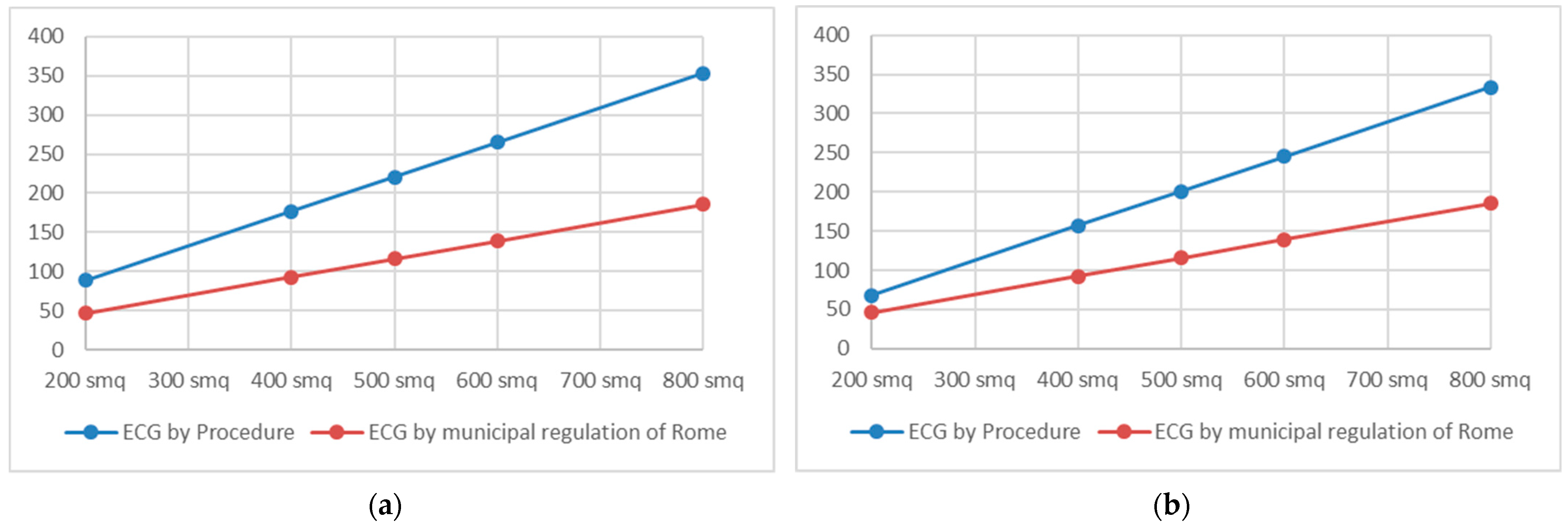
A web-based survey to identify municipal regulations on the ECU, as of 21 July 2021, revealed a sample of 100 municipal resolution that essentially adopt one of the two methods mentioned, but with some variations and applying different coefficients. In most of these cases, the percentage applied by the municipalities to the surplus value generated by the interventions (ECG) is 50% (the minimum required by national law); very few municipalities set a percentage higher than 50% of the ECG and among these the Municipality of Rome (66%) was one of the first to regulate the calculation of the EUC (Resolution of the Capitoline Assembly no. 128/2014).

Basically, the surplus value achievable with the urban variant is obtained through the difference between the TV post-variant and the TV pre-variant (in symbols: TVpost − TVante). According to the classical estimative doctrine and in line with the International Valuation Standards [35], the TV is calculated as the difference between the market value of the building obtainable from the property transformation (MV) and the necessary transformation cost (K). Real estate quotations of the Italian Revenue Agency are often cited as a reference for determining MV, while a “conventional” calculation method for K is generally adopted, using regional price lists or municipal tabular data and fixed percentages for estimating indirect cost items (including the developer’s profit).

Many administrations have then introduced corrective coefficients (generally from 1.50 to 2.00) applicable to the ECU amount in order to direct the building activity towards a sustainable urban development or to incentivise the interventions aimed at: the settlement of tertiary and productive functions, the recovery of disused buildings in the historic centre, and the requalification of buildings and degraded urban areas, thus limiting the consumption of natural soil [36,37].

In other cases, however, the provision of reductive coefficients may lead to determining the ECU to an amount lower than the minimum legal threshold. The Puglia region, for example, provides multiplicative coefficients from 0.80 to 2.00 (depending on the territorial context concerned and the expected urban load) that municipalities may further reduce (through coefficients from 0.2 to 0.4) if intervention is a part of integrated urban regeneration programmes or is a result of architectural project competitions.

This heterogeneity and the evident limits of the calculation mechanism adopted by most of regions and municipalities hinders the effective reform law application [1].

The few ECU assessment models found in the literature [2,38] refer to the TV determination scheme. They calculate the riskiness of the intervention within the promoter’s profit percentage (empirically established, one-off or as the sum of pre-established multi-criteria scores [39]), and determine the discount factor [3] over the entire duration of the transformation (sometimes preordained in 5 years) on the basis of a predetermined rate of interest expense (6%).

Similar models are re-proposed in guidelines adopted by PAs for the economic evaluation of public–private agreements that is aimed at including proposals or projects of relevant public interest in planning. For example, the Municipality of Vicenza [40] refers to art.6 of the Veneto Regional Law no. 11/2004 and recalls in turn guidelines for the evaluation of instruments such as Integrated Intervention Plans used in the Municipalities of Milan, Verona (D.G. no. 659 of 1/06/2004), Rovigo (D.G. no. 20 of 10/02/2005).

The Municipality of Treviso, within the Piano di Assetto del Territorio Territorial Management Plan [41], adopted omnibus guidelines that present a comparative framework of methodological approaches, to evaluate and distribute the public–private benefit, and include also the financial version of the TV, besides the synthetic and non-discounted one.

4. Methods and Material

4.1. Methodologies for Determining Transformation Value (TV)

In the Italian estimative tradition, TV is applied both as an estimative procedure—valid for the generality of market operators—and as an estimation criterion or economic aspect derived, referred to a particular operator as an expression of economic convenience judgments [42].

The International Valuation Standards (IVS) distinguish between market value and values other than market value. The latter are not logically different from the “derived” economic aspects typical of the Italian school such as TV [42]. At the international level, in particular, TV is included in the concepts of “highest and best use” and “use value” [43,44]. It is defined in the IVS [45] as Residual Method.

The Italian estimative tradition defines the criterion of TV of an economic asset (such as an urban area) through the relation:

TV = MV_P − K

(6)

where MV_P (Market Value post-transformation) includes the revenues from the marketing of the goods obtainable with the transformation and K represents the transformation costs, direct (DK: technical construction cost) and indirect (IK: charges and other costs necessary to start and realise the transformation).

The market value of a building area, as a production good, coincides with the TV only in the hypothesis of a perfectly competitive regime and long period equilibrium [46]. The existence of profit is justified both as compensation for the economic risks of production, and as a stimulus to any activity: this profit can be determined practically with reference to the profit corresponding to any activity of an “ordinary” economic operator, or which comparative market experience indicates as most frequent [46].

It is therefore possible to propose the TV formulation, as an analytical procedure for estimating building areas, where the most probable market value of the transformed asset (MV_P) is reduced by the transformation cost (K) including the “normal profit” of the developer (Up) to remunerate his investment, because of the relative risk, and discounting this difference to the time value of the transformation:

TV = MV_P/qⁿ − (K + Up)/qⁿ

(7)

where the discount factor 1/qⁿ = 1/(1 + r)ⁿ is a function of the discount rate r and the time of the normal transformation n (which chronologically shifts the equation terms).

As already noted, in practice the Italian PAs use an ‘timeless’ formula (without the factor qⁿ) to determine the TV and thus to quantify the ECU amount.

The estimation of the MV_P, represented by the revenues from the sale/rental/management of the transformed asset, theoretically requires the analysis of [47]: historical or market data, potential or average income.

In practice, the MV_P is usually determined, synthetically or parametrically, using market data published by official sources or, more rarely, through direct market surveys related to the segment or sector considered.

Without detailed planning, the direct transformation costs (DK) can be derived from:

(a)

Similar interventions using a synthetic-comparative procedure and identifying a final cost (€/sqm, €/cubic metre);

(b)

Price lists of the Public Works Department or published by trade associations (e.g., in Italy published by “DEI, Maggioli” [48]), using parametric costs;

(c)

Summary cost estimate, usually attached to the project or feasibility study.

Indirect costs (IK) are generally derived as a percentage of MV_P and DK. Italian technical literature and municipal regulations concerning the calculation of the ECU use different terms and percentages, but the cost items calculated are substantially similar. By way of example,

Table 1. Quantification of transformation costs (Rome Assembly Decision no. 128/2014).

Cost Items	Calculation Mode	[Average%]
DK = Direct Costs
C0 = technical cost of construction or redevelopment	parametrically 1
IK = Indirect Costs
C1 = adapting cost of the area and connections;	2–5% (C0)	[3.5%]
C2 = urbanisation charges (D.P.R. no. 380/2001)	10% (C0)
C3 = technical-professional and complementary expenses, contingencies;	8–12% (C0 + C1)	[10%]
C4 = marketing charges;	2–3% (MV)	[2.5%]
C5 = borrowing costs on debt D, con qn = (1 + i)n and interest rate I = Spread + (EurIRS or Euribor) 2	D% (C0 + C1 + C2 + C3 + C4) × (qn − 1)
C6 = (gross) promoter’s profit (Up)	15–25% (MV)	[20%]
K = Total transformation cost	C0 + C1 + C2 + C3 + C4 + C5 + C6

Source: elaboration from Rome Assembly Decision no. 128/2014. ¹ using the parametric values €/sqm taken from the Prezziario del Collegio Ingegneri e Architetti di Milano (DEI latest edition available at the evaluation time) for specific intended use of asset. ² Assuming a loan duration of 15 years but considering only a pre-amortisation period of 5 years (n = 1, 2, …, 5) divided as follows: 10% (1st year); 30% (2nd year); 40% (3rd); 20% (4th); 0% (5th).

shows the items contained in the Rome Municipal Decision.

In order to take into account a more detailed distribution of costs and revenues over the time span of the real estate transaction, it is possible to use the DCF [45], wherein the TV corresponds to the Net Present Value (NPV), given by the algebraic sum (Σ) of costs (excluding Up) and revenues—as expected cash flows (CF)—discounted through a factor (1/q^t) according to their time sequence (t) within a suitable duration (n):

$$\mathrm{TV}=\mathrm{NPV}={\displaystyle \sum }_{\mathrm{t}=1}^{\mathrm{n}}\frac{{\mathrm{CF}}_{\mathrm{t}}}{{\mathrm{q}}^{\mathrm{t}}}={\displaystyle \sum }_{\mathrm{t}=1}^{\mathrm{n}}\frac{{\mathrm{CF}}_{\mathrm{t}}}{{\left(1+\mathrm{r}\right)}^{\mathrm{t}}}$$

(8)

This formula, therefore, takes into account the so-called “financial value of time”. Given that the time horizon of these initiatives is at least 5–10 years, even on the basis of the forecast of significant changes over a long period [3,47]: the longer the time needed to generate inflows in order to repay outflows, the higher the risk that the project will not generate the estimated cash flows in the long term [25].

In each case it is therefore decisive to estimate accurately the r-rate, or DR, because while it is difficult to deduce from the market, even small deviations of the rate itself determine appreciable changes in the TV, influencing the ECU amount.

The construction of the discount rate (DR) in the DCF is based on the risk-return concept, also taking into account debt capital [49].

4.2. Methods of Estimating the Discount Rate (DR)

In general, the criteria for estimating DR are based on two fundamental principles: substitutability of the investment and consistency with the expected cash flows [50].

Three techniques for determining the discount rate can be identified as [51]:

• Total expected return;
• Additive return (financial build-up approach);
• Capital cost (WACC).

In particular, the WACC (Weighted Average Cost of Capital) methodology, derived from the corporate field, is the most widely used one in DCF practice [3,23,28,47,49,52]; it determines the DR as the weighted average cost of all financing forms—with equity (k_E) and with debt (k_D)—according to the shares/quantities used (D: Debt, E: Equity) as a debt ratio—or leverage (D/D + E)—assumed at market values and constant for the entire time horizon:

WACC = k_E × E/(D + E ) + (1 − tax rate) × k_D × D/(D + E)

(9)

Since the tax structure of the potential investor is unknown, a pre-tax flow is used, and thus also a rate with the same characteristic; hence the absence of the correction factor (1 − tax rate) [25] which, in the investment assessment, takes into account the tax benefit of deductible financial charges:

WACC = k_D × D/(E + D) + k_E × E/(E + D)

(10)

The market value estimating of an asset, in fact, excludes subjective values—such as the financial structure and capital cost of the investor—but uses market values adopted on average to invest in the given type of asset (in terms of required return on equity, cost of debt and typical financial structure commonly used in the market).

The following paragraph will focus on how to determine the two components of estimating DR as capital cost (WACC), i.e., the financing cost with equity (E) and debt (D).

4.3. The Weighted Average Cost of Capital (WACC)

4.3.1. Debt Price

Assuming that each finance source of a (PPP) project has its own cost, the debt price (Kd) is calculated on the basis of current credit costs, plus a margin to cover the risk of default and operating costs incurred.

Ultimately, the Kd assumed is generally equal to a base rate (EurIRS) plus the Spread [47,52] as remuneration for the major institution depending on the (borrower or) project creditworthiness, as well as the financing model and duration [25]. In addition to the spread, derived from the main Central National Banks, the costs of financing structuring (Fees) are taken into account [28].

4.3.2. Equity Cost

Estimating the equity cost of (PPP) projects is more complex because it is difficult to find benchmarks in the financial markets and the specificities of these transactions make each investment a kind of unicum [25].

Among the approaches that can be used, even jointly, the “orthodox” method [25° VEC,20] refers to the Capital Asset Pricing Model (CAPM) [53].

The CAPM is the reference model in corporate finance and, although it is open to criticism, it is the one that currently allows the most appropriate estimation of the expected return on capital [25] as the sum of two factors (Formula (11)):

Ke = Rrf + β × EMRP

(11)

As regards the practical calculation methods, it should be noted that:

Rrf is the risk-free rate; it is calculated, in practice, by taking as an indicator reference the yield of government bonds (for example, in Italy, the yield: of the BTPs issued by the Italian State or calculated by the Bank of Italy) with a homogeneous maturity with the project time horizon.

β expresses how the project return may vary as a consequence of market variations; it is not easily available, since it depends on the peculiar project characteristics.

EMRP (Equity Market Risk Premium), or MRP, is the compensation for the investor given by the difference between the expected market return (Rm) and the risk-free rate (Rrf).

Since the real estate investment (in PPP projects) is not as easily transferable as a market share quoted, a non-liquidity risk premium can also be taken into account, i.e., an extra remuneration linked to the risk of long-term capital immobilization [25].

Costs related to the structuring of funding, as success and arranging fees are quantifiable, respectively, in the order of 0.7% and 0.9%, or 1.6% overall [28].

The CAPM is extended to the real estate sector [3,23,28,47,49,52] according to the formula:

Ke = Rrf + (β_imm × EMRP) + γ = Rrf + [β_imm × (Rm − Rrf)] + γ

(12)

where: β_imm is the covariance index of the real estate sector and measures the investment return sensitivity to movements in the whole market; γ is the premium for additional risk components that depends on the specific project characteristics (location, type, size, etc.).

In order to determine Rrf, β_imm and MRP, it is possible to refer to datasets used in international valuation practice (Bloomberg, Damodaran, etc.) [52], which make numerous economic and financial data freely available (

Table 2. Official sources and data platforms to determine the components of capital costs: (a) Ke; (b) Kd.

	Factor	Source	Benchmarks
components of Ke	Rrf	National Central Bank; Bloomberg	nominal yields on government bonds with a maturity comparable to the duration of the operation (average reference period)
	EMRP (MRP)	Bloomberg	inferable values for the national market concerned
		Damodaran	Equity Risk Premium (ERP) for the country concerned
	β	Damodaran	Beta of the sector: Real Estate (Development)—Western Europe
components of Kd	EurIrs (o Euribor)	www.Euribor.it (or Il Sole 24Ore, for Italy)	average of the values recorded backwards for a period representative of the market trend
	Spread	Deutsch Bank, BNP Paribas, Credit Agricole, ecc	percentage value determined by the main European banks (estimated around 2%)
		Damodaran	Annual published value for “Western Europe”

).

The estimation of the γ generally requires a market survey of similar real estate development projects, already realised.

In this direction, the Italian Revenue Agency (IRA) has proposed a real estate risk assessment model γ (hereinafter, IRA model) based on the large dataset analysis (42 real estate development projects mainly residential in Rome) through several statistical-economic methods (DCFA, CAPM and Multiple Regression Analysis) [54]. In relation to the market segment investigated and to the available information, this model selects some investment risk factors indicated in the TEGoVA reports [55] and describes them each through a nomenclator with the assignment of a score (risk level), according to a conventional scale of importance: having previously defined the various differentials that characterise each factor, the expected γ of the initiative is given by the sum of the values assigned to each risk component (

Table 3. IRA model to assess the specific risk γ of real estate investment with predominantly residential use.

Specific Risk Factor Levels	Location	Property Size	Building Equipment	Dimensional Factors	Presence of Competitors
	0.0948316	0.0160615	0.0291632	0.0298292	0.062866	Weights
	40.74%	6.90%	12.53%	12.82%	27.01%	% on the total
1	0.18%	0.03%	0.06%	0.06%	0.12%
2	2.01%	0.65%	1.18%	0.82%	2.54%
3	3.83%	1.58%	2.87%	1.78%	6.20%
4	6.59%			2.94%
5	9.35%

Source: Own elaboration by Caravella G.; Lisi G.; Pizzirani F. Costruzione di un modello di valutazione del rischio immobiliare: Fondamenti teorici e prime evidenze empiriche. In Quaderni dell’Osservatorio; Year VIII; Agenzia delle Entrate: Roma, Italy, 2019; pp. 39–58. Available online: https://www.agenziaentrate.gov.it/portale/documents/20143/263933/Quaderni+2019.pdf/dcf95fde-0b75-5e23-a881-2b8fd1cd383b (accessed on 10 July 2021). [54].

), assuming that the level associated with a highest rate of return corresponds to the highest score.

It follows that the γ associated with a generic project can vary from 0.45% (γ_min = 0.18 + 0.03 + 0.06 + 0.12) to 22.94% (γ_max = 9.35 + 1.58 + 2.87 + 2.94 + 6.20) while for intermediate risk values it can be determined as follows:

γ_medium = 3.83% + 0.65% + 1.18% + 1.78% + 2.54% = 9.98%.

(13)

The model’s dataset was subsequently expanded to 90 projects, according to the building type of multi-storey buildings or small villas, and the model itself is susceptible to further development pending its testing [56], given its well-founded approach. On the basis of the discussion initiated with the academic world [57], IRA will extend the study of property risk factors at least to medium-large Italian cities: its aim is to create a national mapping of real estate risk and consolidate the model itself, methodologically and experimentally.

4.4. Calculation of Project Cash Flows

The calculation of Cash Flows (CF) allows the assessment of the project capacity to generate enough liquidity, in the operational phase, to remunerate both the investments and the debt-equity investors in line with their expectations. In the sector literature, these two dimensions are, respectively, defined as: Free Cash Flow from Operations (FCFO), and Free Cash Flow to Equity (FCFE) [25]. The possible growth rate of CF, over this period, can be appropriately related to the expected activity trend of its sector. In view of the uncertain forecasting price trends, a constant price exercise is frequently used (generally adopting the last available price). Alternatively, it is necessary to make assumptions about trend in prices for costs and revenues rather than applying a uniform expected inflation rate (which is probably elusive beyond 3–5 years) [58].

Inflation adjustments rarely apply, fully or partially, to operating costs and revenues, but rarely to investment costs (given the limited duration of the investment phase, even multi-year, compared to the overall project duration) and the debt price (usually estimated as a fixed value) [25].

With regard to expected inflation, it is theoretically equivalent to express flows at nominal or real values, as long as they are consistent with DR [59].

Assuming that DR is gross of interests, it is in fact considered that they incorporate part of the real loss value of capital [56].

In general, DRs are gross of interest charges on debt and subjective income taxes because these would lead to different values for the same real estate property when financing choices and subjective tax situation vary. The exclusion of the tax variable neither influences nor weakens the applied methodology.

4.5. Conditions of Economic-Financial Balance and Contract Renegotiation

The conditions of financial balance of the project/investment are achieved when, in discounted values, the project revenues cover: the investment costs, the operating costs, the capital cost (debt and equity) and taxes.

The occurrence of higher costs or lower revenues, during the agreed projects implementation, implies a renegotiation of the (PPP) contract, which can also be “positive” for the PA if the events (not attributable to the OE) generate extra profitability.

In order to rebalance the Economic and Financial Plan (EFP), even considering different scenarios, it is necessary to realign NPV and IRR to the initial contract levels, maintaining targets also for the project bankability (with DSCR normally not lower than 1.3/1.4 [25]).

The parties may also identify a new balance point, normally no higher than initially agreed, or establish a tolerance value to avoid the EFP revision at each fluctuation of targeted indicators (e.g., ± 0.5% compared to the original project performance) [25].

The agreed variation of the ECU amount can be a further rebalancing lever with immediate impact on the EFP.

5. Experimental Procedure for Determining the ECG

5.1. Variables and Procedure Objectives

The introduction of the ECU not only raised a series of delicate issues in the context of urban transformation interventions, but also raised two substantial questions: (1) the correct evaluation procedure that the PA must use to determine the “surplus value” generated by the interventions (ΔV = Extra Capital Gain); (2) the percentage that must be applied to this surplus value to identify the amount destined to the PA. In this sense, as already highlighted, the mentioned national rule has been implemented by the Regions in controversial ways.

The aim of the proposed procedure mainly responds to the first question, since any definition of the ECU cannot disregard a correct evaluation of the Extra Capital Gain (ECG) representative of the main variable to be considered.

Since the surplus value of the transformation already includes the higher promoter’s profit, it is observed that for the ECG percentages: (i) less than 100% of the ECG, the implementation of the initiative could be considered profitable by the promoter, since the higher cubages that can be realized could determine—net of the ECU destined to the PA—an increase in profit compared to the pre-variant situation; (ii) equal to or higher than 100% of the ECG, the advantage (higher profit) of the post-variant situation would be absorbed by the additional charge, risking even to “erode” the normal profit expected in the pre variant situation (under normal conditions) [60].

Given that the ECG, and the ECU, are closely related to the gross floor area (GFA) to build or redevelop, the procedure aims to achieve the amount of the ECG as the best combination of the factors involved, starting from the urban parameters in derogation: the additional building type areas (BTAi) achievable for each functional destination (residential, tertiary, etc.), together give back the additional GFA compared to the situation pre-variant: they are initially (and reiteratively) assumed as known data of the model such as to: (i) cover the higher transformation costs compared to the situation pre variant, (ii) repay the ECU required, and (iii) satisfy the expected convenience for investors and for the PA.

Just the functional mix to be granted with the variant and the building indexes are crucial variables for the investor’s profit and for the rent determination [9]. Since they represent the morphological composition of the urban area (or the real estate compendium), as object to intervention, they are at the basis of the public–private negotiation [61] and must be contained in the EO proposal (private initiative) or identified by the PA (public initiative), possibly through a market survey.

In practice, area (GFA) and functional mix (BTAi) play the dual role of input and main variables. Once established the main technical–economic–financial quantities of the transformation (unit costs/revenues, expected cash flows and their discount rate)—they can settle the trade-off between the parties with reference to the consequent (reiteratively) determined surplus value.

The analysis of the convenience, from the public and private point of view, is outlined in mathematical terms, comparing the costs and the revenues of the intervention (generally as Free Cash Flow Operative, through the DCF analysis) and their timing, possibly in coherence with the results of the IRA’s research about the market absorption times for the territorial area concerned [55]. Taxes and duties are not considered because they relate to the legal and fiscal profile of the actors involved.

For the purposes of this work, the proposal of a predominantly residential project is assumed and the “conventional” calculation method adopted at local level (Region and Municipality) is maintained for the estimate of the most probable market value MV (with reference to the Real Estate Market Observatory in Italy) and of the project transformation cost K, before and after the variant. In this way, the results produced by the proposed experimental procedure are comparable with the calculation scheme adopted by the municipalities. Among the indicators of the investment evaluation, the net present value (NPV) is used. It is assumed that prices (unit costs and revenues) are constant, except for relevant management components of projects that require assumptions on their annual trend increases: this is based on the sector cost trend as reported by national statistical institutes (ISTAT, for Italy) and the inflation rate estimated by the European Central Bank in the medium-long term. It must always be clear, however, that the estimation procedure inevitably includes uncertain elements, also typical of investment hypotheses, and needs a proper/critical application by the users.

5.2. Structure and Steps of the Procedure

The PA normally verifies the formal conformity of the projects to the General Plan (GP), but it must increasingly assess the substantial performance of the intervention programmes proposed by private operators as a variant to the same GP [6].

The procedure illustrated and implemented below represents a tool that is well compatible with administrative tender procedures, normally initiated by a specific call for tenders. The subsequent phases include negotiation on equal terms between the contracting administration and each economic operator, up to the contract awarding to one or more partners according to the criterion based to consider the economically advantageous offer.

The public valuation perspective assumes an interacting PA that, in examining private parties’ proposals, aims to pursue a balanced weighing of the mutual interests at stake.

The flexible and reiterative nature of the procedure, since it can diversify the factors or the scenarios characteristics, makes it applicable to a wide range of interventions, mainly of a residential nature, and to the various (pre)-contractual phases.

Here, we assume that, at the (private) initiative stage or at an interlocutory stage of a public procedure, the Promoter formulates a proposal to the PA, containing the data reported in

Table 4. Relevant input data of the private proposal to enhance a free area in derogation of the GP.

Data Typology	Parameters per Scenario (S)	Description/Formula 2/Note
Data urban planning	Typology intervention	new building, urban renovation, etc.
	Land Area (of intervention)	LA (mq), (for area)
	Land Building Index	LBIS (smq/sqm or cm/sqm)
	Gross Floor Area (building) 1	GFAS = LBIS × LA
	Building Types Areas	(BTAi)S = [(%i) × GFA]S
Timing (analysis period)	time span transformation	nS (in years); t = generic year of duration n
	time distribution MV, K	[(%MV)t, (%DK)t, (%ICK)t, (%IKR)t]S
Revenue of transformation	Market Value (MV)	(MV)S = Σ(MVi)S = Σ(UMVi)S × (BTAi)S
	average Unit Market Value (UMV)	UMVS = [Σ(UMVi × BTAi)S]/GFAS
Cost of Transformation (K)S = DKS + IKS	Direct Cost (DK)	DKS = [Σ(UDKiS × BTAiS)]
	average Unit Direct Cost (UDK)	UDKS = [Σ(UDKiS × BTAiS)]/GFAS
	Indirect Costs IK = IKCS + IKRS	IKCS = [Σ(%K) × DK]S, IKRS = [(%R) × MV]S
	Extra Charge of Urbanization	ECU
Financial Parameters	Cost of financing/funding	Ke (cost of Equity), Kd (cost of Debt)
	Leverage ratio	D/E

¹ According to the rules of Presidential Decree 138/98, also used to determine Italian Real Estate Market Observatory quotations. ² The analytical translation of technical-urban planning and estimative quantities are derived from the basic principles of the relevant semantic fields.

for both intervention scenarios (ante/post Urban Variant): they will be translated into numerical–monetary terms of the case study (par 5).

Figure 1 summarises the (6) steps of the procedure, which are illustrated in the following paragraphs.

The data proposed by the promoter are redetermined by the PA, in the ante and post scenarios (step 1), and compared with each other (step 2) in order to select the most advantageous values for the PA, as inputs for the calculation system (according to the DCF): it determines the ECU (“reference value”) as the difference of the NPV post/ant Urban Variant (UV) (step 3). By varying the average Unit Market Value (UMV) and the Discount Rate (DR), starting from the values initially selected (step 4), and extending the duration by n years (step 5), the variation tables of the ECU with respect to these three critical variables highlight its sensitivity and therefore the randomness degree of the results obtained. This elaboration (what-if-analysis) may lead to the confirmation of the “reference value”, as the final result, or to the calculating reiteration (step 6), modifying the input data (step 1–2) until this value is considered “reliable”, as the point of risks–opportunities balance between the promoter and the PA.

Step 0—Preliminary data valuation (eligibility and consistency of the proposal). The PA verifies the compliance with the GP of urban planning data proposed by the promoter for the ante-UV scenario and discretionally assesses the admissibility of the post-UV scenario proposed as an exception to the GP (including its duration and the operation timing) if deemed social desirable and consistent with the territorial government strategies.

Step 1—Data verification and determination. If the proposed scenarios are deemed admissible and consistent with the adopted area planning strategies, the PA assumes the timing of the cash flows expected by the promoter (who is responsible for organising the overall building production process) and redetermines for each scenario: direct costs (DK), using unit costs (UDKi)—generally parametric—taken from sector publications or from online applications made available by trustworthy bodies, possibly corrected by coefficients referring to location and environmental context, age, consistency and coherence of the compared work categories (quality level); revenues from the intervention (MV: Market Value) using the average Italian Real Estate Market Observatory quotations (usually in €/sqm) published for the area concerned (or neighbouring/similar areas) and for each building type envisaged by the transformation (or directly assimilated) in the supposed maintenance state. The values as new, if not explicitly stated, are assumed to be the maximum value of the “normal” state of conservation increased by 30%; the economic and financial parameters for quantifying DR, by consulting online official sources and datasets/platforms commonly used at international level, also by means of editable excel files (

Table 5. Sources/references of technical-financial parameters to quantify the DR.

Index	Source		Reference
Rft	Central National Bank		Average yield on government bonds—by residual life span comparable to the analysis period of the transformation—in the year closest to the time of the estimate for a period sufficiently representative of their performance
	es. for Italy: https://www.bancaditalia.it/compiti/operazioni-mef/rendistato-rendiob/ (accessed on 25 July 2021)
β	Damodaran		Factor “Beta” of the “Real Estate (Development)” (Industry name)
	http://people.stern.nyu.edu/adamodar/link “Europe” of Current data set “Levered and Unlevered Betas by Industry” _last accessed: 25/07/2021 (Topic: “Discount Rate Estimation”), downloading Regional datasets (Excel)
MRP	Damodaran		The most recent “Equity Risk Premium” value assigned to the country concerned
	http://people.stern.nyu.edu/adamodar/New_Home_Page/datafile/ctryprem.html or http://people.stern.nyu.edu/adamodar/ click on “Current Data”—“Risk Premiums for Other Markets” (accessed on 30 July 2021)
D/E	Damodaran		“D/E Ratio” of the “Real Estate (Development)” (Industry name)
	download the Regional datasets from http://people.stern.nyu.edu/adamodar/ (see β) (accessed on 2 August 2021)
Eurirs	European Banking Federation		Average of the reference interbank rate recorded backwards from the time of the estimate and with a maturity (years) comparable to the analysis period.
	https://www.ebf.eu (data are published in the main newspapers/magazines specialized in the financial sector (e.g., in Italy: ilsole24ore, https://mercati.ilsole24ore.com/tassi-e-valute/tassi/irs) or can be inferred from other sources/bank institutes, etc.) (accessed on 2 August 2021)
Spread	Damodaran		Last percentage of “Adj. Default Spread” assigned to the country concerned
	http://people.stern.nyu.edu/adamodar/New_Home_Page/datafile/ctryprem.html (accessed on 25 July 2021)
γ	Italian Revenue Agency			IRA Model [54]
	https://www.agenziaentrate.gov.it/portale/web/guest/schede/fabbricatiterreni/omi/pubblicazioni/quaderni-osservatorio (accessed on 16 August 2021)
	Punteggi da stabilire	Factor	Location	Property size	Building equipment	Dimensional factors	Presence of competitors	Total
		Level	L1 (from 1 to 5)	L2 (from 1 to 3)	L3 (from 1 to 3)	L4 (from 1 to 4)	L5 (from 1 to 3)	Σ(L)i

).

Step 2—Data comparison and input selection. By comparing each data or parameter calculated by the PA (^A) with the one proposed by the promoter (^P), it’s possible to select the values that tend to maximise the ECG of the initiative (

Table 6. Data comparison and DCF input selection (^A—administration, ^P—promoter).

Scenario	Unit Direct Cost (UK^A, UK^P)	Unit Market Value (UMV^A, UMV^P)	Cost of Equity (Ke^A, Ke^P)	Borrowing Cost (Kd^A, Kd^P)	Ratio Leverage (D/E^A, D/E^P)
Post (Ante) UV	MIN (MAX)	MAX (MIN)	MIN (MAX)	MIN (MAX)	MAX (MIN)

), as inputs to the DCF, and to determine at the same time: indirect costs (IK), in proportion (in percentage terms) to the selected inputs (MV_P, DK) as defined in the specific municipal regulation; the DR, indirectly, through the WACC method (prudentially without the tax rate):

DR = (ke)/[(D/E) + 1] + (kd) × (D/E)/[(D/E) + 1] = (Rrf + β × MRP + γ)/[(D/E) + 1] + (Eurirs + Spread + Fees) × (D/E)/[(D/E) + 1]

(14)

Step 3—Implementation calculation system. Inserting the selected inputs into the DCF, according to the timing proposed and verified in the first steps, the PA determines the cash flows (CFt) of each scenario, as the algebraic sum of costs and revenues (MV-ΣKi)t for each year (t) of duration (n). Discounting the CFt through the factor 1·[(1 + DR)]^−t by their temporal allocation, the DCF analysis returns NPV and IRR of each scenario: the difference (NPVpost-NPVante) is the potential extra capital gain of the initiative: it derives the ECU (≥50%ECG) as the reference value obtained from the procedure application and comparable with the ECU offered by the promoter.

The discretional assumptions concerning CFt (MV, K) and their discounting (n, DR) are limited, but it is clear they have a strong impact on the NPV and ECU amount. The “reference value” will therefore be confirmed or not as a result of subsequent sensitivity analyses of the ECU to the DR/UMV pair (step 4) and the duration n (step 5). In this way, the structuring of a variability framework of the price-risk-time makes it easier and more consciously possible to validate the reference value that best weighs the critical factors (cost–benefit and duration–risk).

Step 4—What if analysis: ECU as Discount Rate (DR) and Unit Market Value (UMV) changes. Four double input matrices with the same structure are used to determine the ECU variation with respect to the variables DR and UMV: the first two contain, for each scenario, the multiple NPVs corresponding to each DR/UMV pair (obtained by varying their respective base values in the terms indicated in

Table 7. DR and UMV variation range and their step percentage of unit change.

Factor	Min	Max	Range (Max-Min)	Range Discretization	Δ%
DRi	DR(γmin) 2	DR(γmax) 2	δDR = DR(γ = 0.45%) − DR(γ = 22.94%)	2x ≈ (max-min)/ΔR	ΔR = ±0.50%
UMVj	−20% UMV 3	+20% UMV 3	δMV = |40% UMV|	2y ≈ (max-min)/ΔV	ΔV = ±2.50%

¹ UMV—related IKs vary too. ² For the determination of DR(γ_min) and DR(γ_max) refer to Table 3. ³ Double the common area estimate.

). The third matrix contains the multiple ECGij obtained by subtracting from each NPV of the post-UV scenario the analogous NPV of the ante-UV scenario; and the fourth contains the corresponding ECUij, calculated as a percentage of the ECG (

Table 8. ECU values (or similarly ECG, NPVs) as DR-UMV changes.

Scenario POST	DRP-MIN	DRP − vΔR%	DRP (Base Value)	DRP + vΔR%	DRP-MAX
0.80 × UMVP	ECU(min,min)	(…)	ECU(med,min)	(…)	ECU(max,min)	0.80 × UMVA
(1 − uΔV) × UMVP	(…)	(…)	(…)	(…)	(…)	(1 − uΔV) × UMVA
UMVP (base value)	ECU(min,med)	(…)	ECU(med,med)	(…)	ECU(max,med)	UMVA (base value)
(1 + uΔV) × UMVP	(…)	(…)	(…)	(…)	(…)	(1 + uΔV) × UMVA
1.20 × UMVP	ECU(min,max)	(…)	ECU(med,max)	(…)	ECU(max,max)	1.20 × UMVA
	DRA-MIN	DRA − vΔR%	DRA(base value)	DRA + vΔR%	DRA-MAX	Scenario ANTE

Note: u varies between 1 and y; v varies between 1 and x (according to a reasonable range discretization).

). Theoretically, the unitary variations in both costs and revenues (ΔUMV, ΔUK) should be counted as a whole, but, simplifying and considering the costs typically concentrated at the beginning of the real estate investment, only the UMV is assumed as an indicator susceptible to variations along the transformation time span and linked to the reference market volatility.

It should be noted that if the two scenarios differ in risk (DR_P ≠ DR_A) and/or market level (UMV_P ≠ UMV_A), the ECGij will result as the difference between the NPVs held in the first two matrices (NPV_P − NPV_A) and corresponding to the input pairs (DRi, UMVj) reflecting this inequality, i.e., |UMV_P − UMV_A| and/or |DRi_P − DRi_A|.

Step 5—What if analysis: ECU as the time (n) changes. Step 4 is repeated as the total duration increases (n): the four matrices are re-processed for each year of supposed delay, i.e., the operation start is shifted by an equal number of years up to the maximum reasonably assessable delay (at least 3 years) (m). A reasonable discretization of the DR and UMV ranges can facilitate the computational phase and a better expositive synthesis.

Step 6—End or reiteration. The procedure ends if the ECU reference value (step 3) is confirmed as a risks-opportunities balance between the promoter and the PA in the overall frame emerging from the double What if analysis; otherwise, it is repeated from step 1, with new data based on the overall assessments of steps 4–5.

Greater awareness of the PA with respect to the options and sensitive aspects of the investment (e.g., timing) also means reinforcing greater investor confidence by raising the level of shared choices.

6. Application of the Proposed Methodology to a Case Study

6.1. Description and Assumptions of the Case Study

The proposed procedure is applied below to a hypothetical case study under the following assumptions: the promoter–owner proposes to the Municipality of Rome the building of an area in derogation to the GP, raising the Land Building Index (LBI) from 0.2 to 0.3 sqm/sqm and offering a monetary ECU amount equal to 77,000 € (calculated according to the municipal regulation provisions); the intervention is completed in 6 years with the sale of the new built units (housing and, secondarily, commercial-office); the two scenarios differ only in terms of urban planning data (LBIante and LBIpost), resulting in a different dimensional factor (Table 3) of the ante/post UV interventions; it is assumed that prices referring to costs and revenues are constant, and Italian Real Estate Market Observatory quotations are available for the building types foreseen in the intervention area.

6.2. Processing and Procedure Results

On the basis of the promoter proposal (including the UV hypothesis to regulate the proposed transformation), the PA examines the possibility of reaching a negotiated agreement and proceeds to:

Step 0: evaluate the consistency and admissibility of the intervention with respect to its own territorial government policies.

Step 1: once the intervention is considered admissible, assuming the urban planning data proposed by the Promoter, for both ante-UV (as per GP) and post-UV scenarios (compatibly with its own planning strategies). It then redetermines: (i) the gross floor area (GFA) that can be built on the area, using the Land Building Index (LBI) from the GP and from the UV (

Table 9. Urban planning data proposed by the promoter and assumed by the administration.

Data		Measure Unit	Scenario Post	UV	Scenario Ante	UV
Land Area	LA	sqm	(LAP)	5000	LAA	5000
Land Building Index	LBI	sqm/sqm	(LBIP)	0.30	LUIA	0.20
Gross Floor Area	GFA = La × LBI	sqm	(GFAP)	1500	(GFAA)	1000
(1a) Free Housing	GFAFH	sqm	(70% GFAP)	1050	(70% GFAA)	700
(1b) Social Housing	GFASH	sqm	(0% GFAP)	-	(0% GFAP)	-
(2a) Management Tertiary	GFAMT	sqm	(15% GFAP)	225	(15% GFAA)	150
(2b) Commercial Tertiary	GFACT	sqm	(15% GFAP)	225	(15% GFAA)	150
(3) Public Services	GFAPS	sqm	(0% GFAP)	-	(0% GFAP)	-

) for each building type (1. Housing; 2. Tertiary; 3. Public Services); (ii) the transformation direct costs (DK) with reference to the unit costs (UDKi_A) hypothetically indicated by the Prezziario del Collegio Ingegneri e Architetti di Milano (DEI most updated edition); (iii) the revenues from sale (MV) on the basis of the unit values for the same typologies (UMVi_A) equal to the average quotations of the intervention area, published by the IRA—Italian Real Estate Market Observatory for the “optimal” state of maintenance (assuming the values indicated in

Table 10. (a) Transformation direct costs (DK) and (b) sales revenues (MV) per scenario.

(a) Costs 1	Average Unit Direct Cost (UDKi)		Direct Cost (DKi)
Use	Post UV	Ante UV	Post UV	Ante UV
Free Housing	1900 €/sqm	1900 €/sqm	1,995,000 €	2,198,000 €
Management Tertiary	1325 €/sqm	1325 €/sqm	298,125 €	446,250 €
Commercial Tertiary	1140 €/sqm	1140 €/sqm	256,500 €	355,500 €
Total Direct Cost (DK)	1700 €/sqm	1700 €/sqm	2,549,625 €	2,999,750 €
(b) Revenues 2	Average Unit Market Value (UMVi)		Market Value (MVi)
Use	Post UV	Ante UV	Post UV	Ante UV
Free Housing	3140 €/sqm	3140 €/sqm	3,297,000 €	2,198,000 €
Management Tertiary	2975 €/sqm	2975 €/sqm	669,375 €	446,250 €
Commercial Tertiary	2370 €/sqm	2370 €/sqm	533,250 €	355,500 €
Total Market Value (MV)	3000 €/sqm	3000 €/sqm	4,499,625 €	2,999,750 €

¹ Source (hypothetical values): DEI price list 2016. ² Source (hypothetical values): https://www.agenziaentrate.gov.it/portale/schede/fabbricatiterreni/omi/banche-dati/quotazioni-immobiliari (accessed on 28 August 2021).

); and (iv) the factors values (

Table 11. Determination of factors for calculating DR.

Factors	Abbreviations	Value/Percentage	Reference Source
Yield “Rendistato” (May 2021)	Rrf	1.47%	MEF—Dipartimento del Tesoro
Equity Risk Premium	ERP	6.85%	Damodaran
(property sector) Beta	β	0.85	Damodaran
Investiment Specific risk 1	γ-post γ-ante	9.98% (post-UV) 8.82% (ante-UV)	Italian Revenues Agency
Spread	Spread	1.95%	Damodaran
EurIrs 2	IRS	0.40%	Sole 24 ore
Financial leverage	D/E Ratio	95.42%	Damodaran

¹ The two scenarios differ, by hypothesis, only for the Dimensional Factor, from 2.94% to 1.78%, due to the higher GFA realisable with the urban variant. ² A period of 15 years is assumed as a reference, in line with the provisions of the Municipality of Rome’s Regulations for calculating financial charges.

) needed to calculate the DR of the scenarios, or WACC, on the basis of the specific risk γ intermediate (Formula (13)).

Step 2: determine the DR, by assuming in Formula (22) the data recalculated by the PA (as a result of the comparisons shown in Table 6) and the indirect costs (IK:) quantified in accordance with the Rome Municipal Regulation (Table 1). The urbanisation charges are established by the specific municipal tables but, for simplicity, they are calculated as a percentage (5%) of DK (or C₀) [3,8]. For clarity,

Table 12. Revenues (MV) and transformation costs (DK and IK) for ante/post UV scenario.

Revenue and Cost Items			Unit Value (€/sqm)	Post-UV (€)	Ante-UV (€)
REVENUES	MV—Market value of the transformation building product		3000	4,499,625	2,999,750
COSTS	C0 = technical cost of construction or transformation (DK);		1700	2,549,625	1,699,750
	C1 = cost of area adaptation and connections;		59	89,237	59,491
	C2 = urbanisation charges (in art. 16 of D.P.R. n. 380/2001);		85	127,481	84,988
	C3 = professional and complementary expenses, contingencies;		176	176	263,886
	C4 = marketing expenses;		75	112,491	74,994
	C = total capital invested (C0 + C1 + C2 + C3 + C4)		2095	3,142,720	2,095,147
	C5 = financial charges on invested capital (C) 1		73	109,109	72,739
	of which for:	n = 5	D = 10%	16,817	11,211
		n = 4	D = 30%	39,886	26,591
		n = 3	D = 40%	39,419	26,280
		n = 2	D = 20%	12,987	8658
		n = 1	D = 0%	0	0
	K—Transformation Cost for DCF (C0 + C1 + C2 + C3 + C4 + C5)		2167	3,251,829	2,167,886
	C6—Promoter’s profit (20%MV)		600	899,925	599,950
	Total cost according to municipal regulations (C0 + C1 + C2 + C3 + C4 + C5 + C6)		2889	4,151,754	2,767,836

¹ Calculated using the formula: I = C x D x [(1 + i)ⁿ − 1], where: D = Debt (percentage share of debt); n = years of accrual of economic factors: 5; i = Eurirs (15 years) + Spread = 0.40% + 1.95% = 2.35% (interest rate on debt).

shows the financial charges (C₅) and the promoter’s profit (middle value of the range) (C₆) according to Rome Municipal Regulations (Table 1). We assume the γ factor including the illiquidity component and estimate the success + arranging fees as a total of (0.7 + 0.9) 1.6%, as deduced from the sector literature [23].

$$DR=\frac{\mathrm{Rrf}+\left(\beta ·\mathrm{MRP}\right)+\mathsf{\gamma }}{\left(\mathrm{D}/\mathrm{E}\right)+1}+\frac{\left(\mathrm{Eurirs}+\mathrm{Spread}+\mathrm{Fee}\right)·\left(\mathrm{D}/\mathrm{E}\right)}{\left(\mathrm{D}/\mathrm{E}\right)+1}=\begin{array}{c}10.75\%\left[\mathrm{DRp}\right]\\ 10.00\%\left[\mathrm{DRa}\right]\end{array}$$

(15)

Step 3: Calculate the following values: (i) CFt in the two scenarios, according to the time allocation proposed by the promoter and assumed by the PA (

Table 13. Discounted cash flows in the scenario: (a) post-UV (NPV_P) and (b) ante-UV (NPV_A).

Timing (Year)		0	1	2	3	4	5	6
(a) Scenario Post-UV (NPVP)
Revenues from sales	MV	0	0	449,963	899,925	1,349,888	1,124,906	674,944
Construction cost	C0	0	0	637,406	637,406	637,406	637,406	0
Cost of area adaptation	C1	0	0	89,237	0	0	0	0
Urbanization charges	C2	0	25,496	12,748	12,748	12,748	63,741	0
Professional fees	C3	0	0	65,972	65,972	65,972	65,972	0
Marketing costs	C4	0	0	28,123	22,498	22,498	22,498	16,874
Financial charges	C5	0	16,817	39,886	39,419	12,987	0	0
Cash flow	CFt	0	−42,313	−423,409	121,882	598,277	335,290	658,070
Cumulative discounted CFt		0	−38,206	−383,408	−293,684	103,990	305,224	661,847
(b) Scenario Ante-UV (NPVA)
Revenues from sales	MV	0	0	299,975	599,950	899,925	749,938	449,963
Construction cost	C0	0	0	424,938	424,938	424,938	424,938	0
Cost of area adaptation	C1	0	0	59,491	0	0	0	0
Urbanization charges	C2	0	16,998	8499	8499	8499	42,494	0
Professional fees	C3	0	0	43,981	43,981	43,981	43,981	0
Marketing costs	C4	0	0	18,749	14,999	14,999	14,999	11,249
Financial charges	C5	0	11,211	26,591	26,280	8658	0	0
Cash flow	CFt	0	−28,209	−282,273	81,254	398,851	223,526	438,713
Cumulative discounted CFt	CFta	0	−25,644	−258,927	−197,879	74,542	213,334	460,976

); (ii) reference ECG of the real estate transformation (as the difference between NPVpost and NPVante) equal to about €201,000 (much higher than the quantifiable ECG as indicated in the Municipal Regulation, equal to about €116,000), and (iii) ECU (66% ECG) equal to €132,575, i.e., 4.22% of the total investment (Table 13). Therefore, the ECU offered by the promoter, calculated in accordance with the provisions of the Rome municipal regulations (€77,228), would not be consistent already at a first check, by applying the experimental procedure (

Table 14. NPV and ECU calculation according to: (a) the proposed procedure, (b) the Rome Municipal Regulation.

	Scenario	MV (€)	K (€)	NPV (€)	ECG (€)	ECU	(%)	ECU (€)	ECU/NPVP	ECU/K(Post-UV)	ECU/ΔGFA
(a)	Post UV	4,499,625	3,142,720	661,847	200,871	ECG	50%	100,436	15.18%	3.20%	201 €/sqm
	Ante UV	2,999,750	2,095,147	490,976		ECG	66%	132,575	20.03%	4.22%	265 €/sqm
(b)	Post UV	4,499,625	4,151,754	347,871	115,957	ECG	50%	57,979	16.67%	1.40%	116 €/sqm
	Ante UV	2,999,750	2,767,836	231,914		ECG	66%	77,228	22.20%	1.86%	154 €/sqm

), because it is much lower than the law minimum threshold (equal to 50% of the estimated ECG) against an increase (+50%) of the GFA realizable (from 1000 sqm to 1500 sqm). It should be noted that, as a precautionary measure, the DCF includes the financial charges calculated according to the mentioned municipal regulation: this makes the results obtained in the two manners as comparable as possible.

Step 4. Develop the sensitivity analysis by recalculating the NPV of each scenario (Table 14) as DR and UMV (and related IK) change within the ranges and in the terms indicated (

Table 15. Range of variation and increases/decreases (Δ%) of UMV and DR (compared to their base values).

Factor	Minimum Value	Base Value	Maximum Value	Δi% from Base Value
DR	WACC (γ = 0.45%) = 5.89%	10.75% (post-UV) 10.00% (ante-UV)	WACC (γ = 22.94%) = 17.40%	±2.50%
UMV	2700 €/sqm (−10%UMV)	3000 €/sqm	3300 €/sqm (+10%UMV)	±5% UMV (±300 €/sqm)

). For the sake of brevity, both ranges are subdivided equally with three intermediate values (±2.5% for DR, ±5% for UMV), including the respective base value.

The difference between NPV_P and NPV_A, for corresponding levels of “risk” (DR_A and DR_P) and “price” (UMV_A = UMV_P), gives the ECG of the real estate initiative and therefore the ECU (66% ECG) (

Table 16. NPV, ECG, ECU= 66%ECG as UMV and DR changes from base-values (Subscript: A = Ante UV; P = Post UV).

DRP	8.25%		10.75%		13.25%		15.75%			DRP	8.25%		10.75%		13.25%		15.75%
DRA	7.50%		10.00%		12.50%		15.00%			DRA	7.50%		10.00%		12.50%		15.00%
UMVP=A	(a) NPVP, NPVA (€ × 1000)									UMVP=A	(b) ECG, ECU (€ × 1000)
(€/sqm)	Post	Ante	Post	Ante	Post	Ante	Post	Ante	…	(€/sqm)	ECG	ECU	ECG	ECU	ECG	ECU	ECG	ECU
2.700	449	316	373	263	308	218	252	179		2.700	133	88	110	73	90	60	73	48
2.850	608	425	518	362	440	308	373	262		2.850	183	121	1s55	103	132	87	112	74
3.000	766	534	662	461	572	398	494	344		3.000	232	153	201	133	174	115	150	99
3.150	925	642	807	560	704	489	616	427		3.150	282	186	246	163	215	142	188	124
3.300	1.083	751	951	659	837	580	737	510		3.300	332	219	292	193	257	170	227	150

).

In particular, Table 16 shows how the ECG amount (and ECU) is sensitive to the variation of DR and UMV. Specifically, the ECG—and similarly the ECU—increases (decreases) by about 4–5% for each percentage point of increase (decrease) of the UMV, with the same DR and decreases (increases) by 5–7% for each percentage point of increase (decrease) of the DR, with the same UMV (Figure 2).

The overall output produced, within the variation ranges of DR and UMV, shows that the maximum value of the ECG (high UMV, low DR) is about 4–5 multiples of the minimum one (low UMV, high DR) and confirms the considerable influence of these factors on the final result. It is also noted that: (i) each square metre of additional GFA (with the hypothesised functional mix) is equivalent on average to over 260 € of extraordinary contribution (66%ECG); (ii) assuming the same risk level for both scenarios (with DR_P = DR_A = 10.75%), the ECU amount, as a reference value, would be about €145,000 (Figure 3), corresponding to about €290 per sqm of additional GFA: the only difference in risk between the two scenarios—quantifiable in 0.75 percentage points of the DR—thus affects the ECU amount by 8–10%.

Step 5. Develop the same calculations (using the DCFs already set) by shifting the operation start by 1-2-3 years and then maintaining the time distribution of CFt within the 6 years foreseen.

Table 17. ECU = 66% ECG (€x1000) as n [(a) both n_A and n_P; or (b) only n_P], UMV, DR change (Subscript: A = Ante UV; P = Post UV).

	DRP	8.25%			10.75% (base)			13.25%			8.25%			10.75% (base)			13.25%
	DRA	7.50%			10.00% (base)			12.50%			7.50%			10.00% (base)			12.50%
UMVP	UMVA	(a) nA = nP = n									(b) nA = 6; nP = n
(€/sqm)	(€/sqm)	n = 7	n = 8	n = 9	n = 7	n = 8	n = 9	n = 7	n = 8	n = 9	n = 7	n = 8	n = 9	n = 7	n = 8	n = 9	n = 7	n = 8	n = 9
2.700	2.700	80	73	66	65	58	51	52	45	39	66	80	91	14	27	38	−30	−15	−4
2.850	2.850	111	100	91	92	82	73	76	66	58	91	104	114	28	40	49	−24	−13	−3
3.000	3.000	141	128	116	119	106	94	101	87	76	116	128	137	43	52	59	−19	−10	−3
3.150	3.150	171	155	141	146	130	115	125	108	94	141	152	160	57	65	70	−14	−7	−3
3.300	3.300	201	183	166	173	154	136	149	129	113	166	177	183	72	77	80	−8	−5	−2

shows how the ECU changes if the delay: (a) is identical for the two scenarios and (b) concerns only the post-UV scenario, due to huge complexity.

Step 6. As preliminarily noted by way of example, the ECU offered by the Promoter, (about 77,000 €) is not considered fair because it represents only 35% of the ECG determined by the PA; on the contrary, the ECU reference value (about 133,000 €) is sufficiently cautious with respect to its variation range highlighted in previous steps 4–5 and in consideration of the risks–opportunities connected to the prices, yields and duration variability.

The results highlight, on the one hand, the need for the appropriate contextualisation of the public–private conveniences, and on the other, the opportunity offered by a preliminary assessment of them. In the case analysed, the possible market value underestimation (or updating) in the order of 5%, in correspondence with a one-year delay in the work start point (n = 7), would risk compromising the investment sustainability for the promoter: the ECU amount initially established would in fact correspond to the entire ECG generated by the urban variant.

Again, if the scenarios differed only in terms of the achievable GFA (assuming an equal riskiness and timing of the expected flows), the ECG is proportional to the NPV share corresponding to the additional GFA share compared to the total (50% NPVante and 33% NPVpost). This is also evident from the linear trend of the ECG generated by the initiative with respect to the GFA (Figure 2) and according to the procedure implemented: the same trend shows a smaller slope if the ECG is calculated according to the Rome Municipal Regulation.

6.3. Utilities of the Procedure

The procedure described and implemented, referring to areas or buildings and declining in the scenario ante or post event or variant (with-without-principle), responds to different purposes according to the use perspective.

In the case of a private initiative proposal, the procedure may allow

1.

The PA to:

• Evaluate the data proposed by the promoter, compared to those considered “ordinary” with reference to benchmarks and sources (pre-)established in the procedure;
• Verify the feasibility and sustainability of the initiative, giving reasons for its choice or any decision;
• Determine and/or verify a fair cost–benefit distribution of the initiative (in progress, ex ante ed ex post);
• Define the ECU and other essential parameters to be used as the basis for a public tender (which could also follow the proposal acceptance);
• Establish limit or threshold ranges (and possible exemptions) of certain economic/financial parameters that could lead to contract renegotiation;

2.

The EO to define its own best offer, which at the same time generates value for the PA and adequately remunerates the production factors on according to the assumed risk.

When the initiative is launched by the administration, the procedure is designed to:

• Assess the project feasibility;
• Promptly define the overall costs and revenues of PPP operation for the (public) sustainability analysis or further analyses of convenience (e.g., Value for Money) [25];
• Establish the ECU, rent or service charge as the tender basis;
• Draw up the summary PEF within the tender documents and including essential elements useful for the market to formulate offers [25].

It should be noted that the PA is generally unable to estimate the cost structure of the EO and particularly underestimates the financial cost structure; the complex activity of forecasting the project revenues and costs, especially of PPP, is in fact characterised by a strong information asymmetry, between public and private actors: it can facilitate opportunistic behaviour of the EO and therefore penalise the PA [25].

In order to provide the PA with an operational and transparent tool to estimate the surplus differential value generated by the intervention, most of the procedure inputs are derived parametrically from the main sector bulletins or from online databases of proven international use (and easily accessible). This simplification makes it easier to check them and to focus more in-depth analyses on deviations from ordinary average values.

The procedure described is easily pre-set by using the excel application and:

• Determines the ECU amount in a relatively simple way, but more detailed and accurate than the simplified methods used in Italian municipalities, including the critical factors of the TV quantification (and consequently of the ECU).
• Constitutes a potential analysis and assessment tool that, in addition to verifying the data proposed by the promoter, offers the PA useful support in negotiating practices and in different phases of a partnership agreement.
• Introduces elements of flexibility, in the current economic phase, that possibly allow to: (i) extend over time the amounts receivable [1], (ii) include new and updated information; (iii) monitor the variables (to be pre-established) that most impact the profitability (e.g., prices, time) and (iv) simulate alternative scenarios of intervention in order to reduce the uncertainty on its possible outcomes.

7. Conclusions and Perspectives

The process of building the public city involves the definition of compromise solutions, mediating between private profit and public interests.

The need for quality urban development and the sharp contraction of available public resources make it urgent to strengthen the public sector role in negotiations with private operators, land owners and/or developers.

In Europe, this context has generated various legislative provisions aimed at regulating the privatisation of the positive externalities resulting from investments or interventions on the territory, and thus raising more capital for public works.

The Italian law establishing the ECU (Law No. 165/2014), as a value-capture provision, is in line with the most advanced international legislation on the subject, but it is largely disregarded or weakened. In fact, the lack of specific indications regarding the procedures for ECU estimating has resulted in a strong divergence in the valuation approaches envisaged by regions and municipalities. In practice, the supposed division between public and private of the surplus value emerging from urban transformations continues to reward the private sector, land rent, consumption or real estate finance to the detriment of public investment in the city [62,63,64]. Moreover, the information asymmetry that penalises the PA and the relatively low competitiveness of the partnership market, given its complex transactions, may induce the OE to opportunistic behaviour, so as to feed, over time, a certain distrust for PPP forms [25].

In order to facilitate this critical link solution, from the definition phase of a PPP project to the—not infrequent—contract renegotiation, the present work aimed to test and develop an operational tool to overcome the procedural lacks of the national law and the methodological inconsistencies of its application. The article demonstrates the operational effectiveness of the experimental procedure that calculates the ECU by comparing the situations before and after the urban variant [10].

The procedure is validated in the Italian case, being largely conformed to the European and international practice, and can be extended to other international contexts, where the following are foreseen: contractor’s contributions for urbanisation and territorial infrastructure; urban land or buildings requalification (with or without change of use) or free areas edification; programmes or projects (in PPP) which presuppose an ante/post with respect to events transforming the status quo. This is with the aim of: (i) negotiating the building parameters and the additional charges of urban transformations, identifying the intervention advantages, especially in contexts with strong expectations regarding the achievable urban income; (ii) defining effective urban transformations or policies that ensure the PA the adequate payment of urbanisation charges and an “opportune” additional extraordinary contribution (in money or works, such as social housing, parks, etc.), without affecting the initiative attractiveness and financial feasibility for private operators.

Compared to the methods used in practice or in the literature, that do not duly consider the timing and riskiness of interventions, the proposed methodology: (i) duly considers these factors, adopting the DCF and providing simple instructions for systematically estimating the DR; (ii) “measures” the uncertainty and randomness level of the result by using immediately readable scenario analyses and evaluating its robustness within the overall output produced.

In particular, starting from the functional mix envisaged by the urban variant (GFA with uses/destinations) the procedure determines the ECU amount payable to the PA for the benefits balance, making it possible to assess the decision variability with respect to the main transformation factors and their incidence on the financial balance. In this way, even by re-iterating the procedure, the promoter and the PA will be able to evaluate a series of solutions and scenarios (what if analysis) where each hypothesis (urban variance) is associated to the risk that the parties assumes and to the ECU amount (in turn closely related to the real estate values).

As shown in Section 6, the ECU calculated according to the municipal resolution (77,000 €) is not considered fair because it represents approximately one-third of the surplus value determined by the PA and, consequently, it is slightly more than half of the ECU reference value (133,000 €) calculated by the procedure also in consideration of the promoter’s risk level.

The research therefore offers a contribution that can be considered innovative for value recapture and value sharing tools, trying to effectively manage (and to the community benefit) the mechanism of differential urban rent.

The implemented procedure can also be usefully adopted by decision-makers in various contexts: to (re)negotiate urban transformation initiatives (also in PPP) or to define the fair re-sharing of its advantages and burdens when the pre-established parameters change. Used by the PA according to the priority request (also non-monetary), the procedure can facilitate the capital acquisition for new public works, to the local communities’ advantage and to guarantee an adequate remuneration for the private sector.

In the (post-)pandemic crisis that exacerbates an already very uncertain and complex socio-economic context for investors, the use of the proposed estimative procedure appears propaedeutic to strengthen: (i) a different culture of “governing by contract” [65] that overcomes the parties traditional antinomy in support of an effective loyal collaboration and the real mutual convenience for the agreement success; (ii) the operators and PA awareness about the most critical project drivers, starting from the conditions of the real estate market; and (iii) fairness and transparency of decision-making processes, with regard to PPPs and particularly to public action towards investors and the community.

The methodological framework proposed could be useful for programming and implementing urban interventions according to specific political-economic features of reference territory, developed and not. This brings to encourage investments type in the perspective of the sustainable principles based on equitably and social justice. Additionally, by the application to a case-study in Italy, the possibility to implement the estimative method to realize a condition of greater control of the impacts and values generated by settlement interventions can be seen, avoiding inequalities and trade-off values between plot areas in the same of different geographical boundaries.

The potential of the developed procedure could be further tested, also for the (quick) verification of more complex analyses, with respect to: (i) different measures of economic–financial convenience and investment bankability (e.g., IRR; DSCR); (ii) different types of interventions, related to buildings or areas; (iii) different transformation process phases, ex ante/ex post; and (iv) different interactions of subjects (promoter/developer/owner/PA).

In perspective, it could therefore be appropriate to use: parameters that make the sensitive aspects of the procedure objectifiable (e.g., aleatory coefficient of real estate market) [66,67] or that include the inflationary factor and/or revaluation/devaluation of real estate values; additional and better sources or reliable datasets to easily quantify the economic–financial parameters (including the IK); objective functions that can maximise one or the other public-private instance (e.g., social housing share). The ECG amount, in fact, is a decisive and indispensable expression of the public–private negotiation that represents, at least primarily, a monetary quantum (as regulations defines the ECU), but can be translated or transferred into other process entities. In this direction and in order to enhance the model flexibility, it is possible to consider endogenous one or more exogenous variables (e.g., GFA plus functional mix, as objectives).

Future developments may also include methodologies that take into account the critical factors correlations (e.g., Monte Carlo). In fact, given the significant unpredictability of estimation results, it may be useful to integrate traditional valuation methods with generating scenarios tools (i.e., inputs combinations), in order to detect in more detail, the valuation intrinsic component of uncertainty and to determinate relevant inputs [68].

References

1. Crupi, F. Rigenerazione Urbana e Città Pubblica. Il Contributo Straordinario di Urbanizzazione nelle leggi regionali. In Città Contemporanea Gigante dai Piedi d’Argilla; Urbanpromo XVI; Planum Publisher: Torino, Italy, 2019. [Google Scholar]
2. Camagni, R. Il finanziamento della città pubblica: La cattura dei plusvalori fondiari e il modello perequativo. In Urbanistica e fiscalità locale; Maggioli: Ravenna, Italy, 1999. [Google Scholar]
3. Modigliani, D.; Camagni, R.; Dongarrà, A.; Fonti, R.; Messina, G.; Tamburini, M. Definizioni e Determinanti della Rendita Urbana: Metodologia di Calcolo e sue Applicazioni alla Città Metropolitana di Roma; INU Edizioni: Rome, Italy, 2016. [Google Scholar]
4. Falco, E. History of land value recapture in Italy: A review of planning and fiscal measures since 1865. J. Plan. Hist. 2016, 15, 230–245. [Google Scholar] [CrossRef]
5. Benevolo, L. L’italia da Ricostruire. Un Programma per il Territorio; Laterza: Rome, Italy, 1996. [Google Scholar]
6. Curti, F. Le condizioni di sostenibilità del welfare urbano. In Lo Scambio Leale; Officina Edizioni: Rome, Italy, 2006. [Google Scholar]
7. Camagni, R. Risorse per la qualità urbana. In Scenari, Risorse, Metodi e Realizzazioni per Città Sostenibili; Gangemi: Rome, Italy, 2012; pp. 39–52. [Google Scholar]
8. Camagni, R. La riforma della fiscalità urbanistica. In Contributi sulla Riforma Dell’imposizione Locale in Italia; Carocci: Rome, Italy, 2016. [Google Scholar]
9. Oppio, A.; Torrieri, F.; Dell’Oca, E. Il valore delle aree nel negoziato pubblico-privato: Aspetti metodologici e orientamenti operative. Valori e Valutazioni 2018, 21, 87–96. [Google Scholar]
10. Guarini, M.R.; Morano, P.; Micheli, A. A Procedure to Evaluate the Extra-Charge of Urbanization. In Proceedings of the 2020 20th International Conference on Computational Science and Its Applications—ICCSA, Cagliari, Italy, 1–4 July 2020; pp. 981–999. [Google Scholar] [CrossRef]
11. Togni, R.M.; Ferrante, G. Clausole di benefit sharing: Equità ed efficienza nell’affidamento dei contratti di PPP. In Finanza di progetto e Partenariato Pubblico-Privato 2015; Editoriale Scientifica: Napoli, Italy, 2015. [Google Scholar]
12. Micelli, E. Partenariato e Urbanistica. Il cofinanziamento dei servizi e infrastrutture per mezzo degli strumenti di piano. In Governare il Partenariato Pubblico e Privato nei Progetti Urbani; Politecnica Maggioli: Santarcangelo di Romagna, Italy, 2010. [Google Scholar]
13. Gielen, D.M.; Tasan-Kok, T. Flexibility in planning and the consequences for public-value capturing in UK, Spain and the Netherlands. Eur. Plan. Stud. 2017, 18, 1097–1131. [Google Scholar] [CrossRef] [Green Version]
14. Camagni, R. Il finanziamento della città pubblica. In La Costruzione della Città Pubblica; Alinea: Firenze, Italy, 2008. [Google Scholar]
15. Alterman, R. Land Use Regulations and Property Values: The Windfalls Capture Idea Revisited. In The Oxford Handbook of Urban Economics and Planning; Oxford University Press: Oxford, UK, 2012; pp. 755–786. [Google Scholar] [CrossRef]
16. Mittal, J. Self-financing land and urban development via land readjustment and value capture. Habitat. Int. 2014, 44, 314–323. [Google Scholar] [CrossRef]
17. Rebelo, E.M. Land betterment capture revisited: A methodology for territorial plans. Land Use Policy 2017, 69, 392–407. [Google Scholar] [CrossRef] [Green Version]
18. Kim, M. Upzoning and value capture: How US local governments use land use regulation power to create and capture value from real estate developments. Land Use Policy 2020, 95, 104–624. [Google Scholar] [CrossRef]
19. Cardoso, I.M. Análise Comparativa das leis de solos de Países Europeus. In Estudo de Enquadramento para a Preparação da nova Lei do Solo; DGODTU: Lisbon, Portugal, 2011; Available online: https://www.forumdascidades.pt/sites/default/files/lds_estudos-2011_imcardoso_analise-comparativa_0.pdf (accessed on 20 July 2021).
20. Calavita, N.; Mallach, A. Inclusionary housing, incentives, and land value recapture. Land Lines 2009, 21, 15–21. [Google Scholar]
21. Wolf-Powers, L. Reclaim Value Capture for Equitable Urban Development, Metropolitics. 2019. Available online: https://metropolitiques.eu/Reclaim-Value-Capture-for-Equitable-Urban-Development.html (accessed on 20 July 2021).
22. Smolka, M.O.; Amborski, D. Value Capture for Urban Development: An Inter-American Comparison; Lincoln Institute of Land Policy: Cambridge, MA, USA, 2000; pp. 1–28. [Google Scholar]
23. Rubeo, F. Partenariato Pubblico-Privato per lo Sviluppo Urbano, 3rd ed.; Politecnica Maggioli: Santarcangelo di Romagna, Italy, 2012. [Google Scholar]
24. Micelli, E. La valutazione delle convenienze pubbliche e private nei programmi complessi. In Selezione dei Progetti e Controllo dei Costi nella Riqualificazione Urbana e Territoriale; Alinea: Firenze, Italy, 2011. [Google Scholar]
25. Vecchi, V.; Velia, L. Creare Partnership Pubblico Privato: Policy, Contratti e Metodologie; Egea: Milan, Italy, 2020. [Google Scholar]
26. Cassese, S. Istituzioni di Diritto Amministrativo, 5th ed.; Giuffrè Editore: Milan, Italy, 2015. [Google Scholar]
27. Guarini, M.R.; Morano, P.; Tajani, F.; Di Liddo, F. Iniziative di riqualificazione urbana in partenariato pubblico-privato: Un modello per la definizione di liste di priorità temporale. Laborest 2020, 30, 50–56. [Google Scholar]
28. Copiello, S. Progetti Urbani in Partenariato. Studi di Fattibilità e Piano Economico Finanziario; Alinea: Firenze, Italy, 2011. [Google Scholar]
29. Morano, P.; Tajani, F.; Anelli, D. Urban planning decisions: An evaluation support model for natural soil surface saving policies and the enhancement of properties in disuse. Prop. Manag. 2020, 38, 699–723. [Google Scholar] [CrossRef]
30. Commission of the European Communities. Green Paper on Public-Private Partnerships and Community Law on Public Contracts and Concessions; COM 327; Commission of the European Communities: Brussles, Belgium, 2004.
31. Codecasa, G.; Di Piazza, F. Governare il partenariato pubblico-privatostrategie di governo e strumenti del management pubblico nei progetti di riqualificazione urbana. In Governare il Partenariato Pubblico e Privato nei Progetti Urbani; Maggioli: Santarcangelo di Romagna, Italy, 2010. [Google Scholar]
32. ANCE. Il Contributo Straordinario per Maggior Valore nelle Regole di Regioni e Comuni. Available online: http://www.anceaies.it/wp-content/uploads/2016/03/Dossier-Ance-sulcontributo-straordinario-per-maggior-valore-Allegato-contributostraordinario__marzo2016.pdf (accessed on 5 April 2020).
33. Crupi, F. Fiscalità urbana e governo del territorio. Tra integrazione delle riforme e complementarietà degli strumenti. In Il Bisogno di Giustizia nella Città che Cambia; Planum Publisher: Rome, Italy; Milan, Italy, 2018. [Google Scholar]
34. Camagni, R. Il Mistero del “Contributo Straordinario”. ArcipelagoMilano 2019. Available online: https://www.arcipelagomilano.org/archives/51773 (accessed on 20 July 2021).
35. Parker, D. International Valuation Standards: A Guide to the Valuation of Real Property Assets; John Wiley & Sons: Hoboken, NJ, USA, 2016. [Google Scholar]
36. Morano, P.; Tajani, F.; Anelli, D. A decisions support model for investment through the social impact bonds. The case of the city of Bari (Italy). Valori e Valutazioni 2020, 24, 163–179. [Google Scholar]
37. Calabrò, F.; Della Spina, L. New the Technical and Economic Feasibility Project: A Lost Opportunity? The Culture of Evaluation for the Feasibility and Sustainability of Public Works. LaborEst 2018, 1, 3–4. [Google Scholar]
38. Calabrò, F.; Della Spina, L. The public-private partnerships in buildings regeneration: A model appraisal of the benefits and for land value capture. Adv. Mater. Res. 2014, 931–932, 555–559. [Google Scholar] [CrossRef]
39. Calabrò, F.; Della Spina, L. Stima e ripartizione del plusvalore generato dai programmi urbani complessi. In Proceedings of the New Metropolitan Perspectives International Symposium (3rd Edition), Reggio Calabria, Italy, 18–20 May 2016; pp. 227–243. [Google Scholar]
40. Reag, S.P.A. Valutazione Economica degli Accordi Pubblico-Privato per il Comune di Vicenza. Linee Guida per l’Amministrazione Comunale (No.7570—Linee Guida Valutazione, 21/10/2011). Available online: https://www.vicenzaforumcenter.it/file/progetti/108125-887-LINEE_GUIDA_ACCORDI_7570_linee_guida_Comune.pdf (accessed on 10 July 2021).
41. Comune di Treviso. Mappatura dei crediti edilizi e della compensazione. Piano di Assetto del Territorio—Allegato A 2013. Available online: https://www2.comune.treviso.it/pat/PDF/pat/34_R02.A-AllegatoA_Mappa%20crediti%20edilizi%20e%20compensazione.pdf (accessed on 10 July 2021).
42. Manganelli, B. A proposal for a synopsis in real estate appraisal between the Italian doctrine and international valuation standards. Valori e Valutazioni 2017, 18, 9–16. [Google Scholar]
43. Dotzour, M.G.; Grissom, T.V.; Liu, C.H.; Pearson, T. Highest and best use: The evolving paradigm. J. Real Estate Res. 1990, 1, 17–32. [Google Scholar] [CrossRef]
44. Boyce, B.N. Real Estate Appraisal Terminology; Bullinger Publishing Company: Cambridge, UK, 1975. [Google Scholar]
45. International Valuation Standards Council—IVSC. International Valuation Standards; International Valuation Standards Council: London, UK, 2013. [Google Scholar]
46. Forte, C.; De Rossi, B. Principi di Economia ed Estimo; ETAS: Milan, Italy, 1974. [Google Scholar]
47. Agenzia del Territorio. Manuale Operativo delle Stime Immobiliari; Franco Angeli: Milan, Italy, 2011; pp. 475–480. [Google Scholar]
48. Collegio degli Ingegneri e Architetti di Milano. Prezziario-Nuove Costruzioni; DEI-Tipografia del Genio Civile: Rome, Italy, 2021. [Google Scholar]
49. Cacciamani, C. Real Estate, 3rd ed.; Egea: Milan, Italy, 2012. [Google Scholar]
50. Del Giudice, V. Estimo e Valutazione Economica dei Progetti; Loffredo: Napoli, Italy, 2015. [Google Scholar]
51. Hoesli, M.; Morri, G. Investimento Immobiliare; Hoepli: Milan, Italy, 2010. [Google Scholar]
52. Vecchi, V. Le analisi economico-finanziarie per la valutazione e gestione di progetti di PPP. In Finanza di Progetto e Partenariato Pubblico-Privato 2015; Editoriale Scientifica: Napoli, Italy, 2015. [Google Scholar]
53. Sharpe, W.F. Capital Asset Prices: A Theory of Market Equilibrium under Conditions of Risk. J. Financ. 1964, 19, 425–442. [Google Scholar] [CrossRef] [Green Version]
54. Caravella, G.; Lisi, G.; Pizzirani, F. Costruzione di un modello di valutazione del rischio immobiliare: Fondamenti teorici e prime evidenze empiriche. In Quaderni dell’Osservatorio; Year VIII; Agenzia delle Entrate: Roma, Italy, 2019; pp. 39–58. Available online: https://www.agenziaentrate.gov.it/portale/documents/20143/263933/Quaderni+2019.pdf/dcf95fde-0b75-5e23-a881-2b8fd1cd383b (accessed on 10 July 2021).
55. The European Group of Valuers’ Associations—TEGoVA. Rating Europeo della Proprietà e del Mercato. PAM (Property and Market Rating). Una guida per il valutatore. Available online: https://www.isivi.it/pamIT.pdf (accessed on 10 July 2021).
56. Caravella, G.; Lisi, G.; Pizzirani, F. Il contributo dell’OMI all’evoluzione del modello di valutazione del rischio immobiliare. In Quaderni dell’Osservatorio; Year IX; Agenzia delle Entrate: Roma, Italy, 2020; pp. 92–108. Available online: https://www.agenziaentrate.gov.it/portale/documents/20143/2994404/06+caravella_lisi_+pizzirani+VISTO+SI+STAMPI.pdf/ee082ed5-786a-a3c7-8c7c-3676fc22d3cb (accessed on 10 July 2021).
57. Guerrieri, G.; Iacobini, M.; Caravella, G.; Lisi, G.; Pizzirani, F.; Cartapati, E.; Manganelli, B.; Gabrielli, L.; Morano, P. Il Progetto di Monitoraggio e Analisi delle Operazioni di Sviluppo Immobiliare dell’Agenzia delle Entrate, Workshop Presentation and Debate; Videoconference: Roma, Italy, 2021. [Google Scholar]
58. Florio, M. La Valutazione degli Investimenti Pubblici. I Progetti di Sviluppo nell’Unione Europea e Nell’esperienza Internazionale, 2nd ed.; Franco Angeli: Milan, Italy, 2003; Volume 1. [Google Scholar]
59. Lanzavecchia, A. L’analisi finanziaria degli investimenti immobiliari. In Real Estate, 3rd ed.; Egea: Milan, Italy, 2012; pp. 331–352. [Google Scholar]
60. Morano, P.; Tajani, F.; Anelli, D. Urban planning variants: A model for the division of the activated “plusvalue” between public and private subjects. Valori e Valutazioni 2021, 28, 31–48. [Google Scholar] [CrossRef]
61. Bravi, M.; Fregonara, E. Promozione e sviluppo immobiliare. In Analisi dei Processi e Tecniche di Valutazione; Celid: Torino, Italy, 2004. [Google Scholar]
62. Camagni, R. Verso una Riforma della Governance Territoriale: Area Vasta e Controllo della Rendita Fondiaria e Immobiliare. Available online: https://storicamente.org/quadterr2/camagni.htm (accessed on 24 July 2021).
63. Nesticò, A.; Guarini, M.R.; Morano, P.; Sica, F. An economic analysis algorithm for urban forestry projects. Sustainability 2019, 11, 314. [Google Scholar] [CrossRef] [Green Version]
64. Guarini, M.R.; D’Addabbo, N.; Morano, P.; Tajani, F. Multi-criteria analysis in compound decision processes: The AHP and the architectural competition for the chamber of deputies in Rome (Italy). Buildings 2017, 7, 38. [Google Scholar] [CrossRef] [Green Version]
65. Valaguzza, S. Collaborare Nell’interesse Pubblico; Editoriale Scientifica: Napoli, Italy, 2019. [Google Scholar]
66. Tajani, F.; Morano, P.; Di Liddo, F.; Locurcio, M. An innovative interpretation of the DCFA evaluation criteria in the public-private partnership for the enhancement of the public property assets. New Metrop. Perspect. 2019, 100, 305–313. [Google Scholar] [CrossRef]
67. Morano, P.; Rosato, P.; Tajani, F.; Manganelli, B.; Di Liddo, F. Contextualized property market models vs. generalized mass appraisals: An innovative approach. Sustainability 2019, 11, 4896. [Google Scholar] [CrossRef] [Green Version]
68. Porzio, C.; Sampagnaro, G. L’investimento immobiliare. Valutazione, Rendimenti, Asset Allocation; Bancaria Editrice: Rome, Italy, 2007; Chapter 5. [Google Scholar]
Figure 1. Workflow of the proposed procedure for determining the ECU.
Sustainability 13 10958 g001
Figure 2. ECG trend (€ × 1000): (a) as risk level (DR) changes; (b) as market values (UMV) changes.
Sustainability 13 10958 g002
Figure 3. ECG trend as the gross floor area (GFA) varies: for (a) DRA = DRP (= 10,75%);(b) DRA < DRP.
Sustainability 13 10958 g003