Article

Kabul River Flow Prediction Using Automated ARIMA Forecasting: A Machine Learning Approach

1
Department of Civil and Environmental Engineering, Universiti Teknologi PETRONAS, Bandar Seri Iskandar, Perak 32610, Malaysia
2
Department of Civil Engineering, Sarhad University of Science and Information Technology, Peshawar 25000, Pakistan
3
Polytechnic Institute, Far Eastern Federal University, 690000 Vladivostok, Russia
4
Institute of Civil Engineering, Peter the Great St. Petersburg Polytechnic University, 195291 St. Petersburg, Russia
5
Department of Theoretical Mechanics and Resistance of Materials, Belgorod State Technological University Named after V.G. Shukhov, 308012 Belgorod, Russia
6
National Institute of Transport, NIT-SCEE, National University of Sciences and Technology, Islamabad 44000, Pakistan
7
Centre for Intelligent Signal and Imaging Research (CISIR), Electrical and Electronic Engineering Department, University Teknologi PETRONAS, Bandar Seri Iskandar, Perak 32610, Malaysia
8
Department of Civil Engineering, COMSATS University Islamabad Wah Campus, Wah Cantt 47000, Pakistan
9
Department of Electrical Engineering, Sarhad University of Science and Information Technology, Peshawar 25000, Pakistan
*
Authors to whom correspondence should be addressed.
Sustainability 2021, 13(19), 10720; https://doi.org/10.3390/su131910720
Submission received: 11 July 2021 / Revised: 6 August 2021 / Accepted: 10 August 2021 / Published: 27 September 2021
(This article belongs to the Collection The Impact of Digitalization on the Quality of Life)

Abstract

:
The water level in a river defines the nature of flow and is fundamental to flood analysis. Extreme fluctuation in water levels in rivers, such as floods and droughts, are catastrophic in every manner; therefore, forecasting at an early stage would prevent possible disasters and relief efforts could be set up on time. This study aims to digitally model the water level in the Kabul River to prevent and alleviate the effects of any change in water level in this river downstream. This study used a machine learning tool known as the automatic autoregressive integrated moving average for statistical methodological analysis for forecasting the river flow. Based on the hydrological data collected from the water level of Kabul River in Swat, the water levels from 2011–2030 were forecasted, which were based on the lowest value of Akaike Information Criterion as 9.216. It was concluded that the water flow started to increase from the year 2011 till it reached its peak value in the year 2019–2020, and then the water level will maintain its maximum level to 250 cumecs and minimum level to 10 cumecs till 2030. The need for this research is justified as it could prove helpful in establishing guidelines for hydrological designers, the planning and management of water, hydropower engineering projects, as an indicator for weather prediction, and for the people who are greatly dependent on the Kabul River for their survival.

1. Introduction

In ancient times, cities were established on the banks of rivers so that their inhabitants could take advantage of the opportunities offered by the river in terms of food, trade, and defence, and the same is applicable in this era of advancement as well [1,2]. Water is necessary for human existence. River water is a source of life for the domestic, industrial, irrigational, and energy sectors [3]. River basin management is a scientific and technical area of study and involves several intricacies because of the various features of particular rivers and their offshoot branches, and land drained by the application of this study [4]. Therefore, it becomes fundamental for engineers to understand the likely behavior of rivers.
The behavior of river water is often unexplainable and unexpected. However, water behavior can be studied and controlled by structural (dams, reservoirs, and barrages) and non-structural (disaster prevention, response mechanisms, and floodproofing) measures. Based on past values, hidden information like the flow of water at a specific time can be revealed using forecasting techniques, which can help early response actions and prevent disasters [5]. Water level and runoff forecasting is a measure of the non-structural type that is essential for modelling natural hazards [6]. Forecasting the water flow of a river is directly related to the developmental activities in nearby regions of the country as it is used in the planning of the cities, the management of river basins, the making of dams, the calculating and controlling of risks related to floods and droughts, and for supplying water for household usage and generating power [7].
The Kabul River originates from the mountains of Hindu Kush and covers about 700km distance before joining the Pakistan water system [8]. The catchment area of the Kabul River in Pakistan is 14,000 km2, while 62,908 km2 lies in Afghanistan, which makes the overall catchment area 76,908 km2 [9]. The Kabul River has an overall basin area of 87,499 km2 [10]. Although the Kabul River originates from Afghanistan, yet it faces water shortage due to the lack of adequate infrastructure of water storage due to the perpetual war [11].
Apart from the Kabul River, other major rivers of Pakistan enter the country from India. As the upper riparian discharge comes under the jurisdiction of India, Pakistan cannot control the water level to fulfill its water requirement [12,13]. This scenario makes it even more important for an agricultural country like Pakistan to plan for increasing its efficiency in the present and future water flow. If Pakistan fails to acknowledge the behavior and importance of the Kabul River, it will face a similar situation of water scarcity like Afghanistan. Hence, both countries (Pakistan and Afghanistan) are largely dependent on agriculture using the Kabul River water. Figure 1 illustrates the river’s origin and its basin location. It is clear that the river originates in Kabul and extends into Pakistan.
The existential threat to the Kabul River is the change imposed by climatic conditions, which have also made the forecasting of river water flow essential because disturbed rainfall patterns have already started to seriously affect the availability of water [14]. Climatic conditions are getting worse day by day, and weather anomalies have direct effects on rivers like the Kabul River. It is estimated that precipitation will decrease by 50% in the Kabul River basin towards the end of this century, which will produce floods of unforeseeable flow and will negatively impact streamflow dynamics [15]. It is also expected that the Khyber Pakhtunkhwa province of Pakistan will be severely affected in terms of the economy and water crisis by 2080 and that the water crisis will result in a considerable decrease in wheat and maize production due to climate change [16]. The people dependent on the Kabul River Basin have been greatly affected by the temperature rise and the shifting of precipitation patterns; moreover, the melting of a glacier in the Hindu-Kush region created havoc in the 2010 floods, which caused considerable damage to the Pakistan economy (855 billion Rupees) and dispersed 20 million people residing near the banks of the river [17,18]. It is estimated that 20% of the precipitation will decrease due to the shift in monsoon season, which, combined with the effect of melting glaciers, will affect millions of people’s existence, as has already been seen in the 2010 floods, in which a significant fertile area was lost due [19].
As the operation of dams is based on the river flow, the Warsak Dam is one of the most important dams of Pakistan in terms of irrigation and energy generation; it is necessary to study the past inflow and outflow to enable forecast the future values, which could help in meeting the water demands of the country [20,21]. Concerning Pakistan, the Kabul River serves as a lifeline for providing safe and drinkable water for 2 million people of Peshawar city and its subregions. Pakistan built the Warsak dam in 1960 on the Kabul River, which generates 243 MW hydropower [22]. Any increase or decrease in the water level of the Kabul River will threaten the balance of life in Pakistan and will result in catastrophic consequences. For example, the floods in the Kabul River happen two times a year, once due to the snowmelt from April to September and secondly as a result of monsoon torrential rainfall in August [23]. With the increase in global warming, the snow melts quicker, and the discharge in the river results in floods. It is estimated that every 1.5 °C or 2 °C rise in temperature results in a 34% or 43% increase, respectively, in runoff from the upstream Indus basin [24]. In the 2010 floods in the Indus river basin, 5.4-million-acre land was lost, 2200 people lost their lives, and 14 million people were left homeless, which resulted in the loss of 43 billion USD [25]. Similarly, any decrease in the water level of the river can adversely affect the system of the agricultural activities in Pakistan as the agriculture sector was the fifth-highest contributor to Pakistan’s overall Gross Domestic Product (GDP) in 2020, and 35.89% of its people are employed in this sector [26].
Human activities like hydropower structures, an explosion in population, a heavy amount of silt, inadequate rainfall annually, unregulated urbanization, illegal settlements, and unapproved water channels from this river have caused a reduction in its water level. Therefore, in terms of its importance for human existence and increased water demand, it is necessary for Pakistan to limit its future water demand and flow [27,28].
Keeping in mind the importance of the above discussion, this study aims to forecast the flow of the Kabul River till the year 2030. To better prepare for recurring natural flood vulnerabilities and avert monetary losses and casualties, possible future changes in flow rate intensity in the Kabul River basin should be analyzed. The objective of this study is to use an effective learning algorithm that could accurately predict and evaluate the different patterns of water levels based on various periods. Another objective of this analysis is to help the upstream technicians of the reservoir by providing a better forecasting tool for the prediction of the expected water levels using the Automatic ARIMA model. The achieved objective will be significant to the relevant authorities because it will help them to plan socio-economic developmental activities efficiently to enable them to cater for future needs, provide water-restraining structures in case of floods, and prepare strategies for water disasters, and it will help relief workers to reduce irreversible human and economic losses.

2. Literature Review

Numerous studies have been conducted to forecast river flow around the globe. Previously, hydrological events were forecasted using conventional methods to predict runoff discharge, capacity, and streamflow of water-level; however, machine learning (ML) is now increasingly being used in hydrological forecasting [29,30]. The term ML implies that machines analyze, cluster, extract complex linkages, and make decisions without programming [31]. The added advantage of using ML is its ability to determine the patterns of the input data and produce output results by analysing the complex structures hidden in the data [32]. The data-driven forecasting models as used in this study are based on the historical data of the water levels, including runoff volumes, storage capacity, and river discharge. This approach includes the use of statistical data as input variables to measure the extent of water flow using output variables [33]. Various algorithms like artificial neural network (ANN) and adaptive neuro-fuzzy inference systems (ANFIS) were used to forecast the water level using hydrological variables like temperature, wind, and evaporation. The water level data from 2007 to 2011 of Chahnimeh Reservoirs in Zabol, Iran was used for analysis. It was found that the ANFIS model was better at predicting the future values of water levels compared to ANN due to it more closely fitting the original values [34].
Various ML models like support vector machine (SVM) ANN, ANFIS, and generalized regression neural networks (GRNN) were used for estimation of the water reservoir level in Millers Ferry Dam on the Alabama River in the USA. When the results were compared to moving average (MA) and autoregressive moving average (ARMA), it was found that ANFIS model 5 output results were more promising due to the lowest value of mean absolute error (MAE), R2, and mean squared error (MSE) [35]. Some researchers used semi-hybrid models like Wavelet-based Artificial Neural Network (WANN) and Wavelet-based Adaptive Neuro-Fuzzy Inference System (WANFIS). The daily water level of the Andong dam in South Korea was forecasted using these two semi-hybrid techniques. The results were expressed as the comparison of the accuracy of these two methods. It was concluded that both methods tend to accurately forecast the conventional models and can yield better efficiency results in the daily water level analysis [36,37]. A least-squares SVM (LSSVM) is another type of intelligent algorithm that was used for the prediction of daily water level Yangtze River in China based on the water level of data from 2010–2016. Based on the lowest value of root mean squared error (RMSE), index of agreement, and mean absolute percent error (MAPE), the improved LSSVM method tends to provide useful figures for hydrological levels [38]. As Pakistan has constructed the Warsak dam over the Kabul River, electricity generation greatly depends on the water level in this river. Hence, hydroelectric consumption was forecasted based on 53-years-worth of data in Pakistan. Methodologically, the autoregressive integrated moving average (ARIMA) model with (p,d,q) values of (9,1,7) was selected for forecasting. The results revealed that hydroelectric consumption will increase 1.65% annually, with a cumulative increase of 23.4% till 2030 all over Pakistan [39].

3. Methods

This study used an ML approach to perform the forecasting. In this study, the methodology was followed by the collection of the hydrological data from 1961–2005. For this purpose, the time series was checked for stationarity using Augmented Dickey Fuller (ADF) test. The ADF test was first invented by David Dickey and Wayne Fuller in 1979 and tests the time series for the null hypothesis of the presence of unit root test [40]. The mathematical expression for ADF is given by:
Δ y = α + β t + γ y t 1 + δ 1 Δ y t 1 + + δ p 1 Δ y t p + 1 + ϵ t
where α is constant, β is coefficient of time trend, p is the lag order, and ϵ t is the error term. After selecting the appropriate lags of order p, the test is executed for the null hypothesis γ = 0 [41]. If the time series has non-stationarity, then the stationarity can be achieved using regression or differencing until the time series become stationary.
The concept of ARIMA was first developed by an electrical engineer named Norbert Wiener et al. in 1930–1940. It consists of three parts called autoregressive (AR), integrated (I), and moving average (MA) [42], whereas ARIMA was first put into use in time series for modelling forecasts by Box Jenkins in 1970 [43]. Since then, the use of ARIMA has found wider application in the fields of engineering, economics, hydrology, and social analysis [44]. The first general form of ARMA was given by Peter Whittle in 1951 [45], which can be shown as:
X t = c + ε t + i = 1 p φ t X t 1 + i = 1 q θ i ε t i
where ε t is regarded as a white noise term and ϕ and θ are regarded as the coefficients of the time series.
The mathematical form of AR (p) and MA (q) is given below in Equations (3) and (4), which were given by [46]:
AR (p), p (number of autoregressive terms)
yt = c + β1 yt−1 + β2 yt−2 + β3 yt−3 + … + βp yt−p + εt
It is a case of multiple regressions, including lagged values of yt as predictors. It is referred to as AR(p), and p indicates AR model of order (p)
MA (q)
yt = c + εt + α1 εt−1 + α2 εt−2 + α3 εt−3 + … + αp εt−p
MA (q), q (number of moving average terms), where d is the times of differentiation.
An automated ARIMA tool was used, which allows the users to identify a suitable ARIMA specification and to perform the forecast for the time series. Automated ARIMA tool is not only limited to ARIMA modelling but also considers a variety of modelling procedures, and the selection of ML models along with its orders were identified. Based on the selected models, the model with the lowest Akaike Information Criteria (AIC) or Bayesian Information Criteria (BIC) was selected.
AIC was first used by Hirotugu Akaike in 1971 [47,48]. AIC calculates the prediction error, which measures the quality of a statistical model with other relative models [49]. It can be expressed mathematically as [50]:
AIC = 2   k 2   ln ( L ) ^
where k stands for estimated parameters in the model and L ^ is the maximum value of the likelihood function. For a given set of models, the model with the lowest AIC is selected based on the goodness-of-fit measure. AIC also has a penalty system that discourages overfitting and hence improves the goodness-of-fit. Similarly, BIC (also known as Schwarz information criterion, SIC) appeared in the 1978 paper, which was developed by Gideon E. Schwarz [51]. In the case of BIC, the formula is similar to AIC but the difference is in a penalty for a different number of parameters. AIC has a penalty system of “k”, while penalty in BIC is ln k [52]. The BIC can be expressed as [53]:
BIC = k   ln   ( n ) 2   ln ( L ) ^
where k is the number of parameters estimated by the model, n is the number of data points, and L ^ is the maximized value of the likelihood function of the model.
AIC checks the quality of each model relative to other models and thus becomes a means for model selection. Mathematically, AIC and BIC (Bayesian information criterion) differ slightly only in terms of penalty for the number of parameters. For AIC the penalty is 2k, whereas for BIC it is ln(n)k. BIC is also a model selection criterion in which the model with the least BIC value is selected. In comparing AIC and BIC, the performance of AIC was found more satisfactory than BIC [52]. It is argued that BIC is the best fit for true model selection for which AIC is not appropriate. This is because when selection is done by considering BIC as the base, the probability of the true model comes to be 1 as n → ∞, which is less than 1 in the case of AIC. Yet, the advisors of AIC claim that it is a negligible issue, as there is no “true model” available in the overall set [54,55,56]. If the models do not consist of the best fit, the analysis part would be repeated by selecting different lags for the automated ARIMA tool. After the model was proposed by the tool, the residual error analysis was performed to check the accuracy of the output of the mathematical model. Among many validation procedures, this study used an out-of-sample validation test to check for the identification and estimation of the model suggested by the automated ARIMA tool. The concept of an out-of-sample validation test is to compare the fitting of the portion of the original data set with the forecasted data set model. Finally, forecasting was performed for the year 2011–2030. The accuracy of the forecasting and error analysis was performed using R2, and error analysis was done using root mean squared error (RMSE), mean absolute error (MAE), and mean absolute percentage error (MAPE).
RMSE is the square root of the sum of all squared differences between the predicted and actual errors [57]. RMSE shows the range of residual spread. It can be expressed mathematically as [58]:
RMSE = i = 1 N   ( P r e d i c t e d A c u t a l ) 2 N
where N = number of observations and i = variables along with predicted values and actual values.
MAE is regarded as one of many measures that are used in a forecast analysis. It is the measure of error between paired observations showing identical occurrence [59] or it is the average of all absolute error terms [60]. It is mathematically expressed as [61]:
MAE = 1 N i = 1 N | y y ^ |
where N = total number of data points and   sum   of the absolute value of the residual y y ^ .
MAPE is the measure of correctness of the forecast [62]. It is expressed in percentage. Mathematically, it can be shown as [63]:
MAPE = 1 n t = 1 n | A t F t A t |
where n is the number of observations, t is the number of variable terms, A t is the actual value, and F t is the forecasted value.

3.1. Data Collection

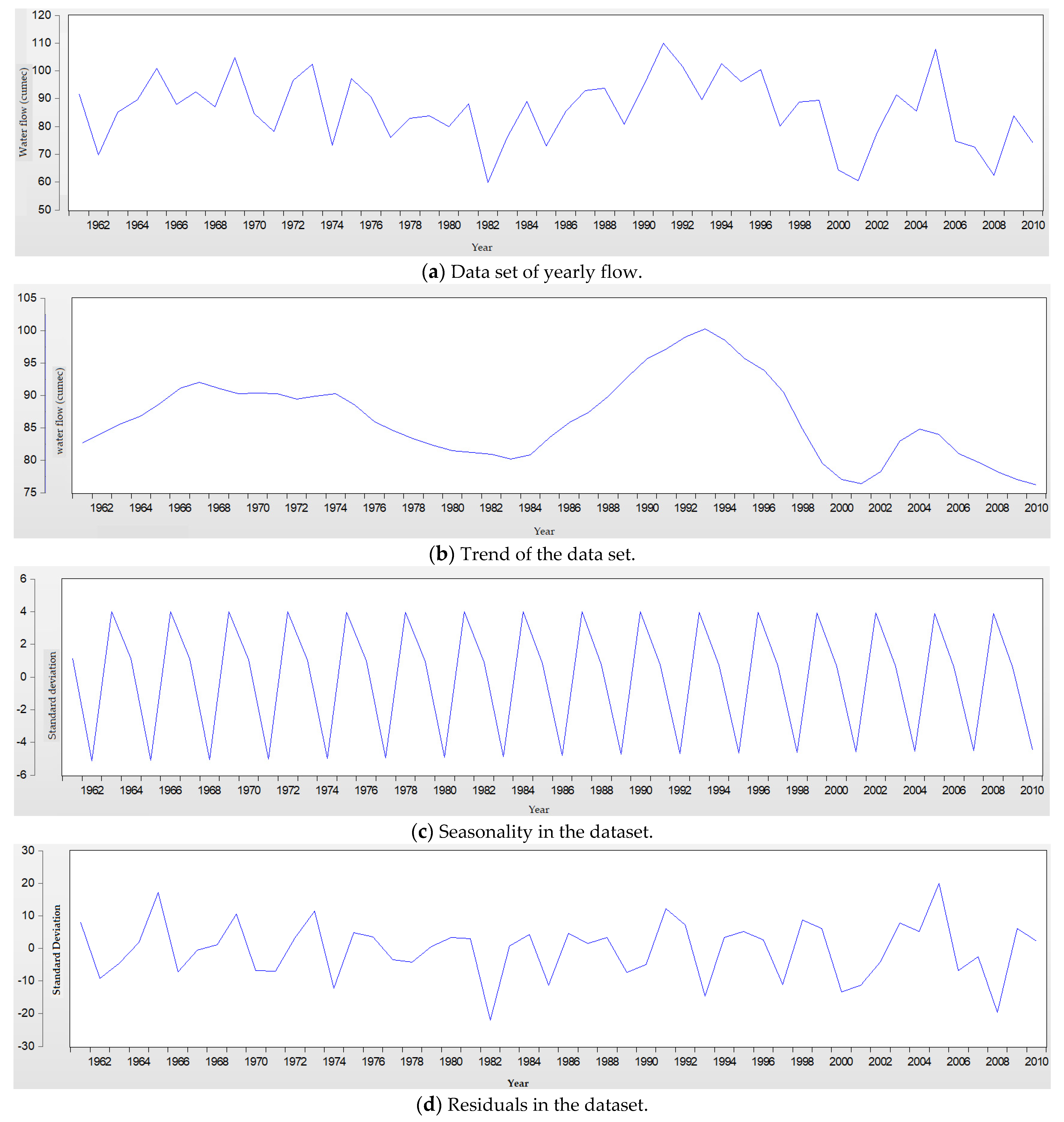
The water flow data were collected of the Kabul River in Swat, a city of Khyber Pakhtunkhwa (KP) Province, Pakistan. The historical data were gathered by the Water and Power Development Authority (WAPDA), a Government Department from the year 1961 to 2005. Afterward, they discontinued collecting the data, where a private consultant with the name AGES collected the data from 2006 to 2010. The seasonal decomposition was performed to analyze the data set that could reveal useful information about the time series. It was found that the highest recorded value was 110 cumecs in 1991, and the second-highest value of 107.78 was measured in 2005. The lowest reading was 59.97 cumecs in 1982, as shown in Figure 2a. Figure 2b shows the trend in the data set. Figure 2c illustrates the seasonal factor present in the time series, and Figure 2d signifies residuals present in the data.

3.2. Forecasting Using Automated ARIMA Tool

In this study, the data of the water flow of the Kabul River was collected and forecasted through the time series method by using software named EViews. EViews is an outstanding interactive program that is the best fit for detailed data analyses [64]. EViews allow forecasting using the Automated ARIMA forecasting feature, which is timesaving in comparison to the traditional programming languages. The term “automated ARIMA” feature selects the model among the AR, MA, ARMA, ARIMA, and seasonal ARIMA models, and it does not mean that this feature will only consider the ARIMA model. For this time series forecasting, the ARIMA model has been used. There are several tools available for linear time series forecasting, but the body of knowledge credits ARIMA as the most suitable one [5]. The ARIMA model contains autoregressive (AR), integrated (I), and moving average (MA). The AR part describes the relationship between present and past observations, the MA part represents the autocorrelation structure of error, and the I part represents the differencing level of the series [65]. ARIMA is one of the most powerful and successful linear statistical models for time series forecasting [66]. Research made by Valipour and Banihabib [67] showed that in comparison with ARMA (autoregressive moving average), the ARIMA model is better than ARMA because it can make time-series stationery in the training and forecasting phase [68]. It can transform the non-stationary data into stationary data. Nevertheless, Yu and Lei [69] believe that to decrease the element of uncertainty and increase the predictive performance, the combination of different types of models is recommended, i.e., the hybrid approach.
The reason for using the Automated ARIMA tool is, firstly, the selection of appropriate values for p (number of autoregressive terms), d (differences required to achieve stationarity), and q (moving average terms). As the ARIMA algorithm consists of (p,d,q) the determination of (p,d,q) is a laborious and time-consuming task, but the Automatic ARIMA function will select the best fit model automatically based on the lowest values of the selected parameters like AIC or BIC. Secondly, the ARIMA modelling accounts for the missing data in the time series. As there is missing data from 2010–2020 in the time series, this modelling technique could compensate for the missing data based on the previous readings. Although many factors come into play that could affect the water flow in the river, the basic reason for using the ARIMA tool is to predict the missing data without considering those factors that could lead to uncertainty in the results. The estimation of missing data help the engineers, designers, and flood controlling department as they seek to include the missing data from this study in their implementation. It has been proven that the missing hydrological data can be computed from the estimation of the fitted models using ARIMA [70,71]. Finally, the use of ARIMA has been well document in hydrological analysis. ARIMA has been used with full confidence in the analysis of water quality [65], rainfall [69,72], runoff [73,74], river discharge [65,75], drought [76,77], monthly streamflow [78,79], and groundwater anomaly [80].
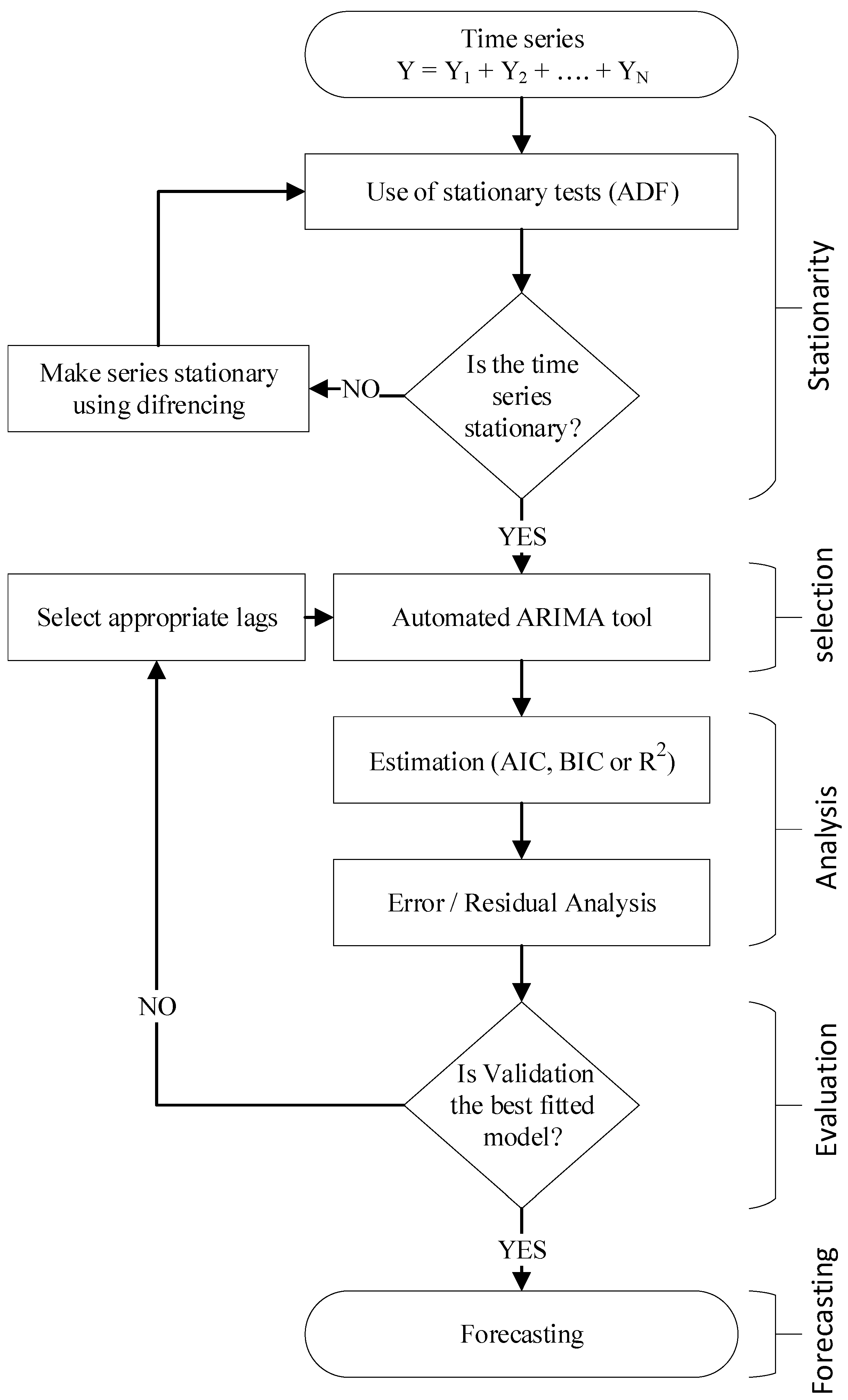
Figure 3 shows the flowchart of the methodology followed. Firstly, the hydrological time series is obtained. Then, the stationary is checked using the ADF test. The stationarity can be achieved using differencing. The Automated ARIMA tool is incorporated to identify the models for analysis. A model is selected based on the lowest AIC and BIC value. The error/residual analysis is performed to check the accuracy of the selected mathematical model. If the validation fails to satisfy the parameters of the best-fitted model, the analysis is repeated for a different model selection using appropriate lags. The study further proceeds with the forecast.

3.2.1. Automated ARIMA Forecasting

The automatic model selection specification for the ARIMA model can be divided into four steps:
  • Using raw or transformed data, such as logs of the dependent variable.
  • Selection of appropriate level of integration of the dependent variable.
  • Evaluation of the exogenous regressors.
  • Selection of the order of the ARMA model using the evaluating technique.
Automatic forecasting automatically takes steps i, ii, and iv. In each step, the user selects the exogenous regressors, hence the name is Automatic ARIMA instead of Automatic ARIMA. Any time series, y t uses ARIMA (p,d,q) if [81],
D   ( y t ,   d ) = β   X t + υ t
υ t = ρ 1   υ t 1 + + ρ p υ t p + θ 1 ε t 1 + + θ q ε t q
where the exogenous variable X t is a constant term and υ t is the seasonal ARMA term. In this case, forecasting can be made using the dependent variables AR, integration, and MA, which can be selected using evaluation techniques. The estimation methods in EViews make use of three information criteria types: Schwarz Criterion (SIC or BIC), Akaike Information Criterion (AIC), and the Hannan-Quinn Criterion (HQ). Based on these criteria, the number of terms of ARMA is selected [81].
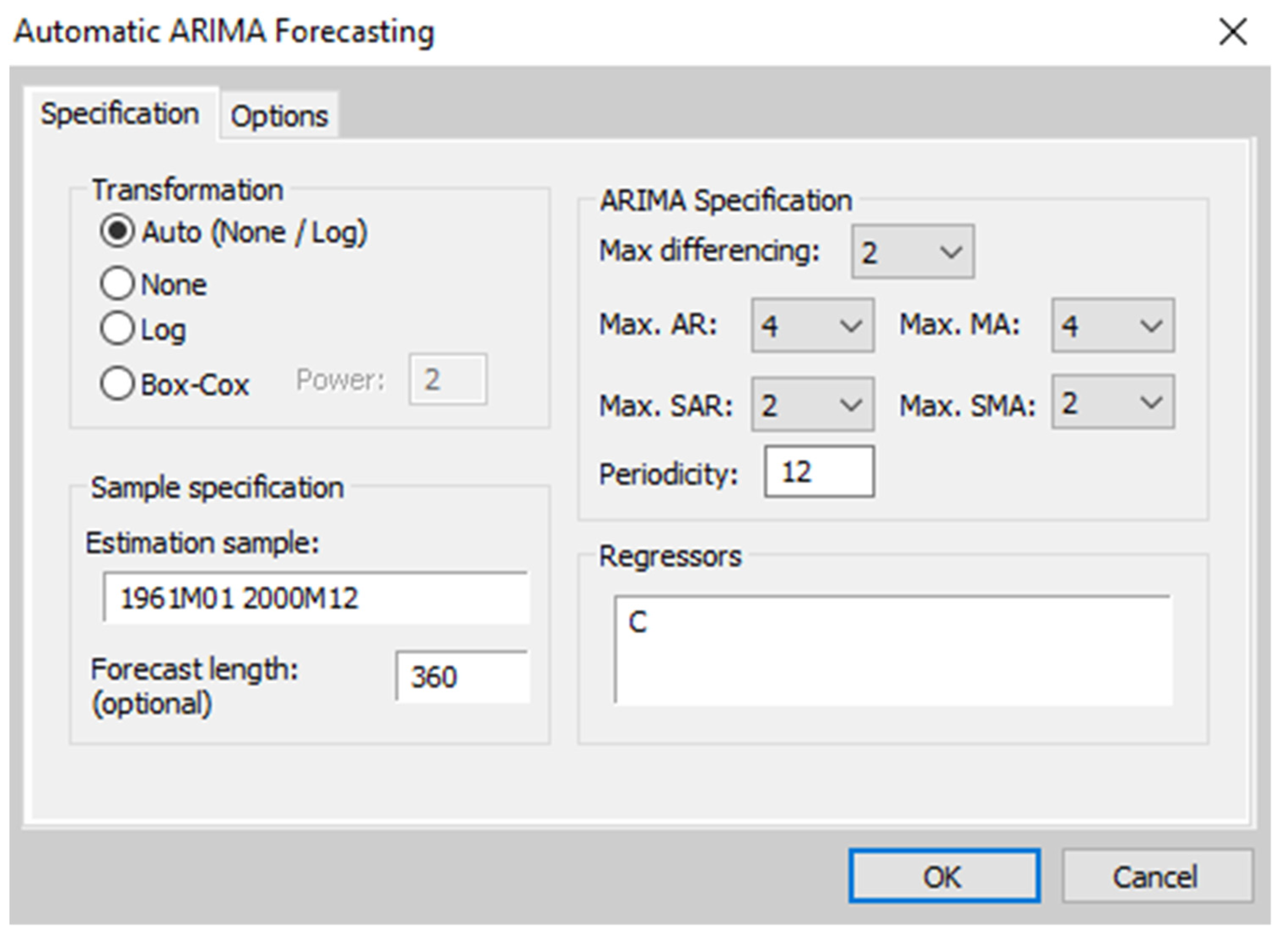
Before performing the analysis, the data need to be split into train and test data. For this purpose, the month-wise data from the year 1961 to 2000 was selected as train data and data from 2001 to 2010 was selected as the test data. Automated ARIMA forecasting is a feature offered within the EViews where a user needs to provide the maximum autoregressive, differencing, and moving average value. The automated ARIMA parameters are shown in Appendix B.
It can be observed that in this analysis the maximum AR value was taken as 4, maximum differing was taken as 2, and maximum MA was taken as 4. As the data show seasonality (S), maximum SAR and SMA were taken as 2.

3.2.2. Model Validation

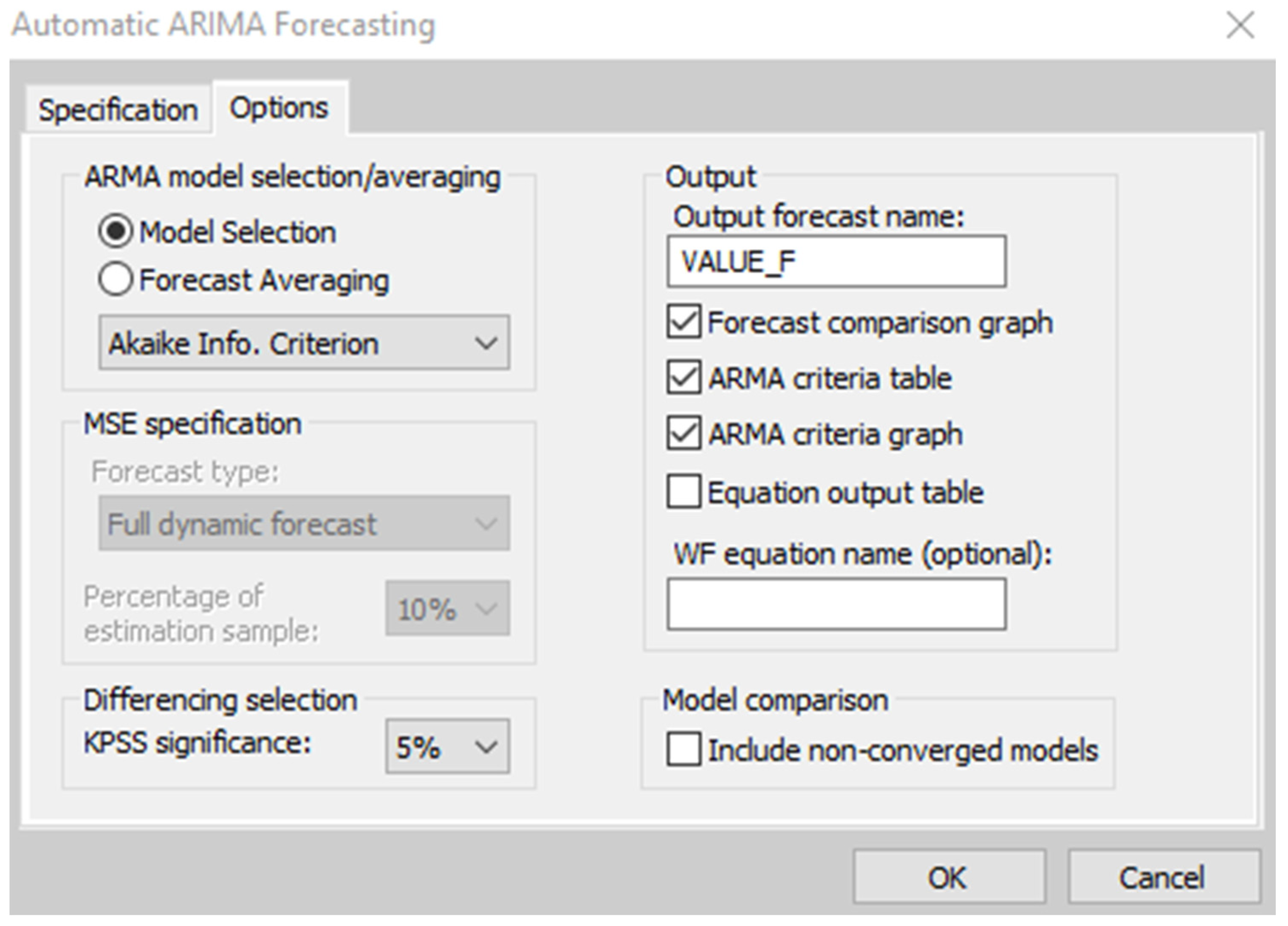
With the automated ARIMA forecasting feature, various ARIMA models are run where the best model needs to be separated. In this regard, the model selection was based on Akaike Information Criterion (AIC) where the lowest value shows the best-fitted model. The model validation features are shown in Appendix C.

4. Results

4.1. Summary of ARIMA Forecasting

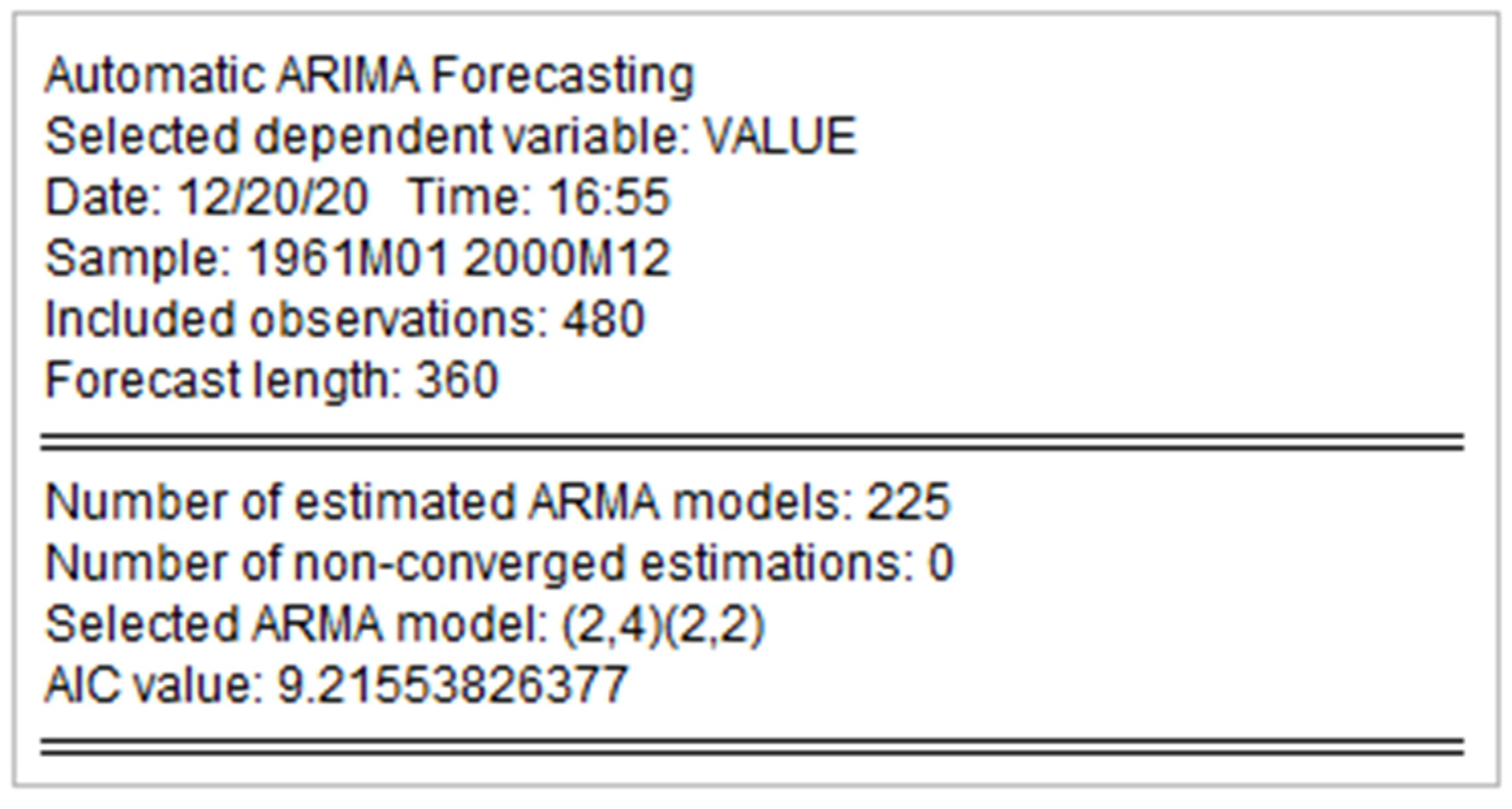
Out of 600, 480 observations were taken as train data. Overall, 225 models were run where the best ARMA model came as (2,4)(2,2) based on AIC value, which was equal to 9.216. A summary of the ARIMA forecasting is provided in Figure 4.

4.2. Comparison of Forecasted and Actual Data

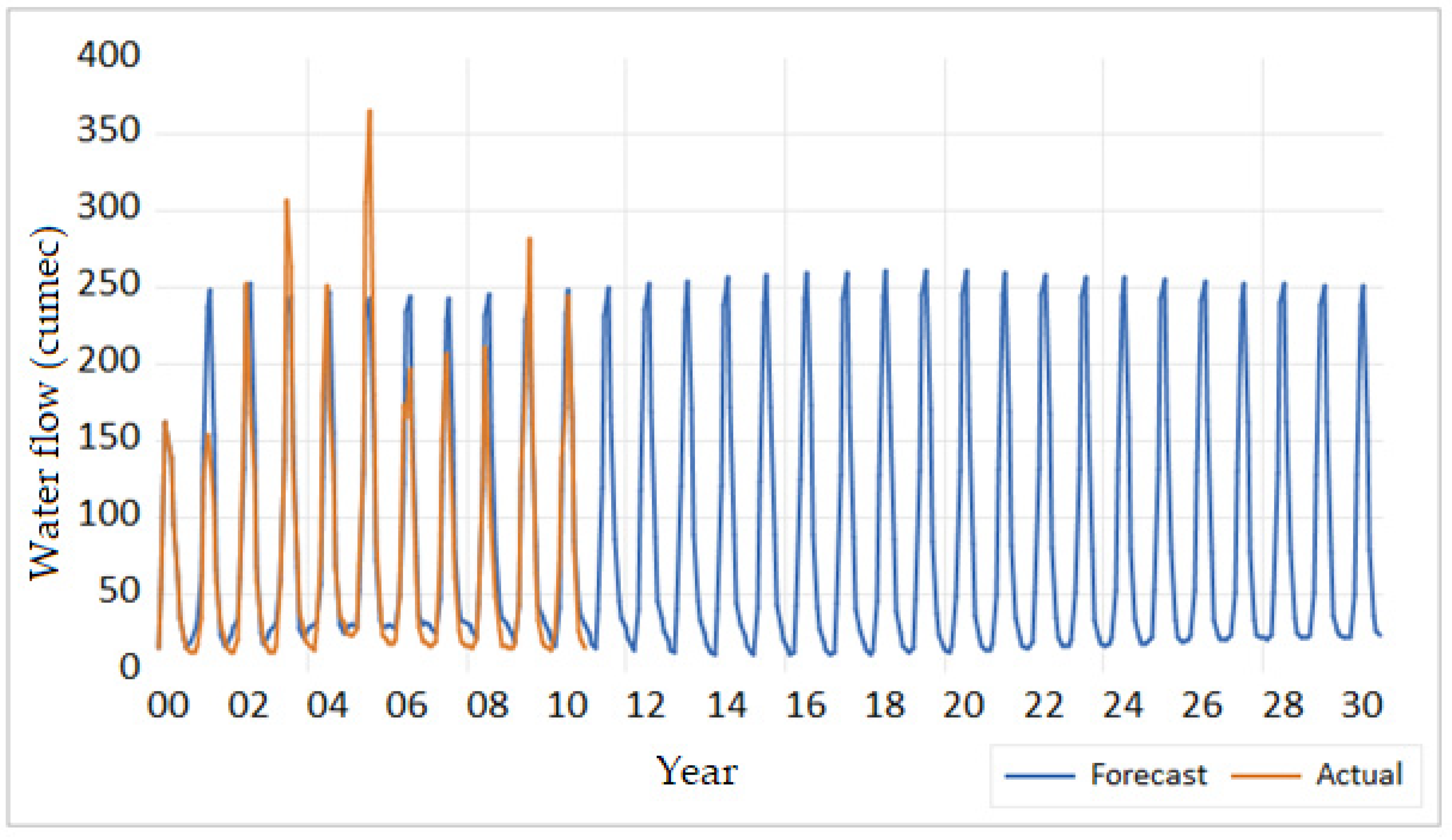
Forecasted and actual data have been compared in Figure 5. The actual data is given for a period of ten years, i.e., from 2000 to 2010. Out of these ten years, the data for the first five years was provided by WAPDA and the data for the remaining five years was provided by AGES. This set of data was selected for the category of test data too. Taking this test data as a reference set, the future forecast for the remaining 20 years was made possible. It can be seen in Figure 5 that actual and forecasted values lie close to each other with a few deviated values. Once it was made sure that actual and forecasted values lay in the proximity of each other, the water flow for the remaining years was forecasted. The reason for ARIMA predictive method, firstly, is that it could cover the missing values, which are essential for future analysis. Secondly, in case of a significant weather shift, this analysis could prove useful to the engineers and designers to improve the capacity of the flood control devices in case of a significant anomaly in the Kabul River. The forecasted values indicate the flow of the river provided the water level due to melting of the glacier and weather shift, and the basin condition of the river remained the same throughout the analysis period. This forecast was produced irrespective of the weather anomalies that are subject to persistent change in the future.
There are many validation methods, and out-of-sample is one of them. The concept of this validation is to withhold a portion of sample data for identification and estimation and then conduct the forecasting for the remaining hold-out data to determine the presence of the errors within the sample fitted data and the forecasted data. In this case, the validation period was selected from 2000–2010 and the forecasting was performed from 2011–2030.
In the light of Figure 5, a peak of the actual water level at 370 cumec can be seen, while the forecasted plot indicates a marginal increase over 250 cumec. The difference between the actual and forecasted value is due to the reason that the ML algorithm estimates the time series value of 12 months and produces output in the form of the average of the past data.
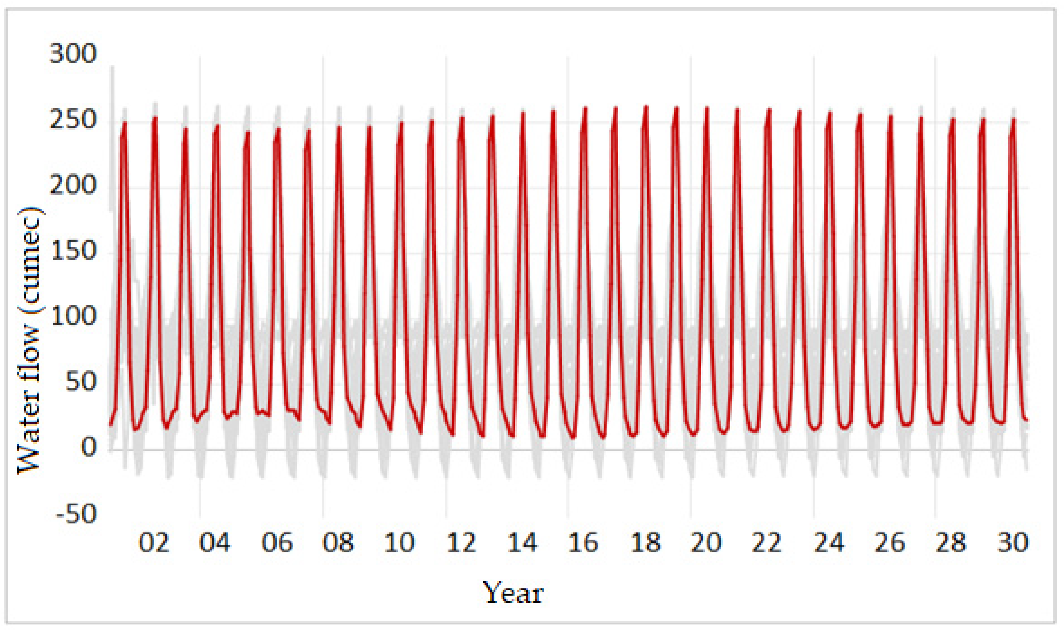
Figure 6 illustrates the comparison of all-inclusive model sets. The transparent graph lines in the background represent the graph lines for 225 simulated models, whereas the graph line highlighted in the red graph line denotes the selected model (2,4)(2,2). It is evident that out of all the ARMA models, model (2,4)(2,2) has the least values, which is why it was selected as the best option.

4.3. Best Fitted Model (AIC)

Appendix A gives the details of the overall 225 ARIMA models. AIC value range is from 9.215538 to 10.26662, whereas BIC value range is from 9.319883 to 10.31879. The model selection is based on the AIC value, and as mentioned above, model (2,4)(2,2) is the selected ARIMA model that has the least AIC value of 9.215538. Different values for models (2,4)(2,2) have been highlighted in Appendix A. The BIC value of this selected model is 9.319883, and the HQ value is 9.256554.
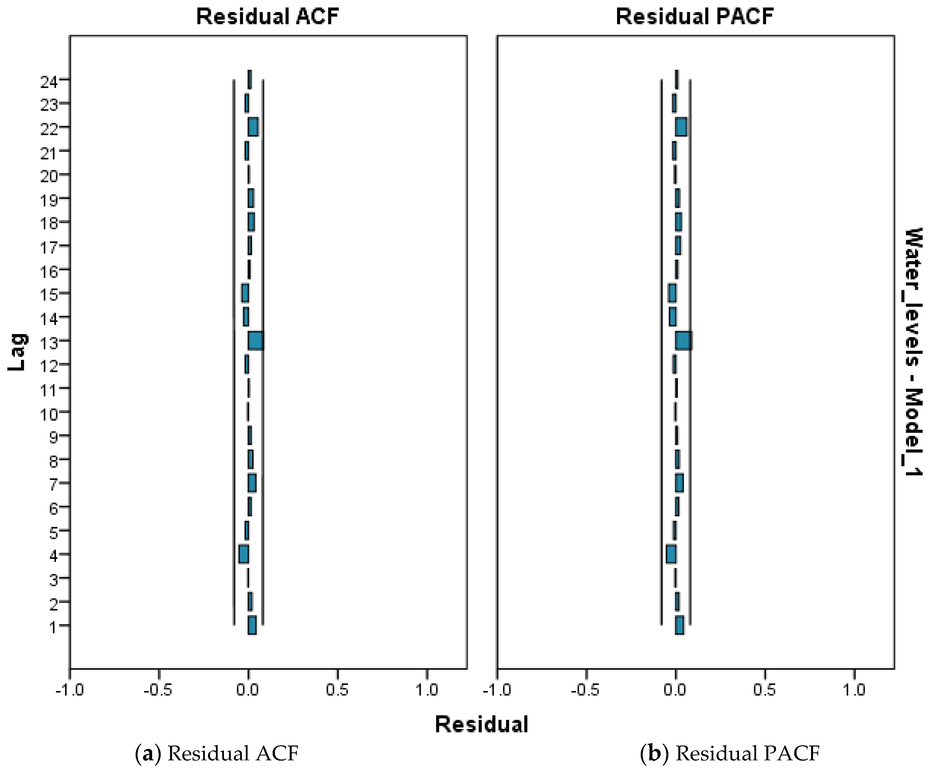
The residual autocorrelation function (residual ACF) and residual partial autocorrelation function (residual PACF) plots were used to determine the residuals in the selected model. As evident from Figure 7a,b, the residuals are randomly scattered, showing the best fit for the selected model of forecast along with the absence of autocorrelation in the residuals. The vertical lines represent the 95% confidence interval (CI), whereas the blue blocks show the number of lags selected to determine the behavior of residuals. The residual ACF and residual PACF plots show that no lags deviate from the CI and are near to zero, which indicates that the residuals are independent and the model has accurately forecasted the time series.
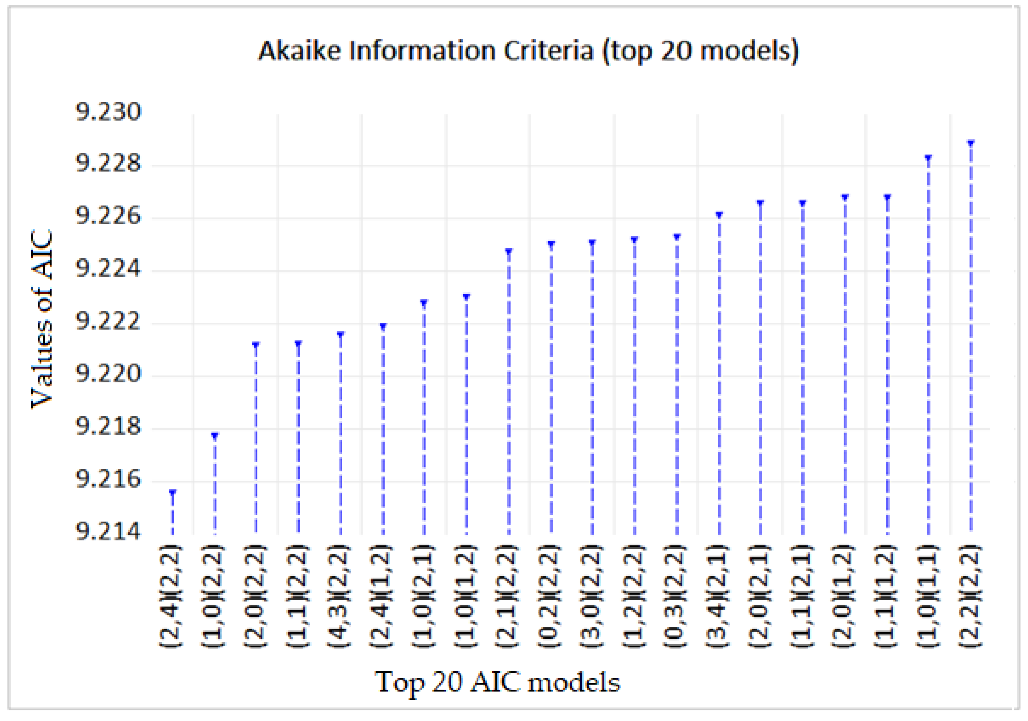
Figure 8 shows the top 20 models with the least values of Akaike information criteria (AIC). Y-axis represents the AIC values from 9.214 to 9.230, and X-axis shows the top 20 models. Overall, the values of these models increase in ascending order. Among these 20 models, the lowest value belongs to the selected ARMA model and the highest value is of model (2,2)(2,2). Models # 3 and 4; models # 10, 11, 12, and 13; and models # 17 and 18 have diminutive difference in values.

4.4. Water Flow Forecasting

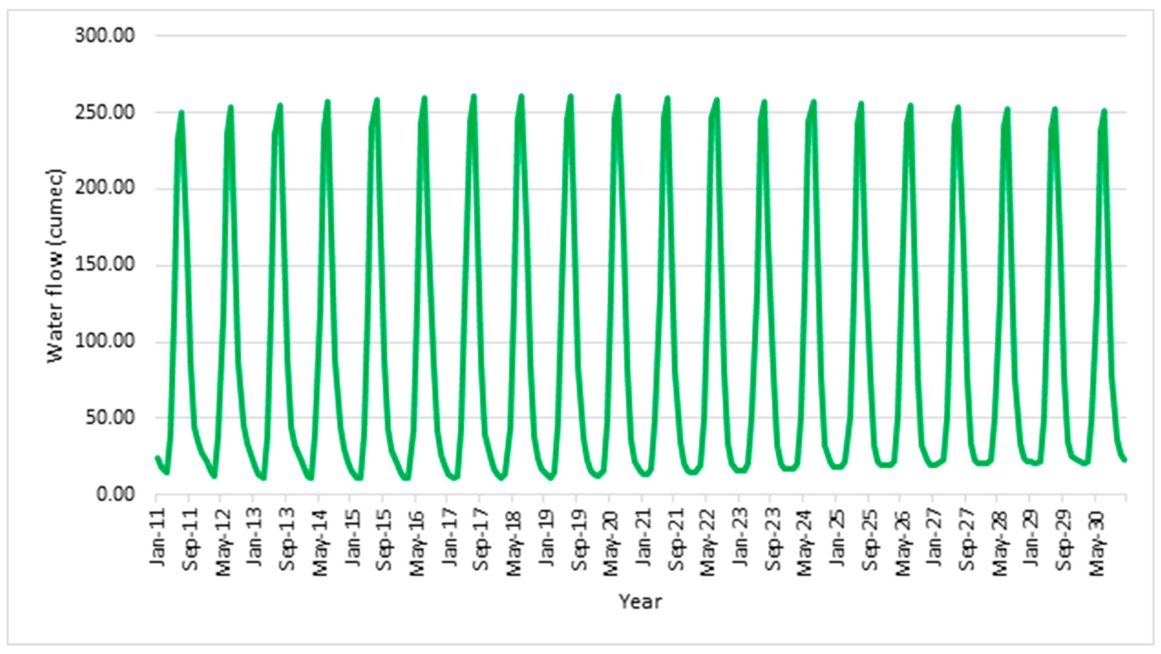
Figure 9 gives the forecasted water flow values from the year 2011 to the year 2030. Y-axis shows the water flow in cumec, and X-axis shows two readings for odd years and a single reading for even years. The forecasted values have been derived from the train data and the test data sets. The predicted water flow is either 250 cumecs or slightly above it. The water flow starts to increase from the year 2011 till it reaches the peak value in the year 2019–2020 and then decreases gradually to about 250 cumecs till 2030.
It should be noted that the automated ARIMA tool considers all linear models, and the selection of ARMA over other models is performed based on the lowest AIC value. Moreover, this analysis used linear models for analysis; therefore, the trend of the dataset is different from the trend of the generated linear results. Additionally, the automated ARIMA tool accounts for the missing data with less error due to its linear behavior. These results predict that the water flow will remain the same if the current condition of the water flow, basin, and drainage remains the same through the forecast period from 2011–2030.
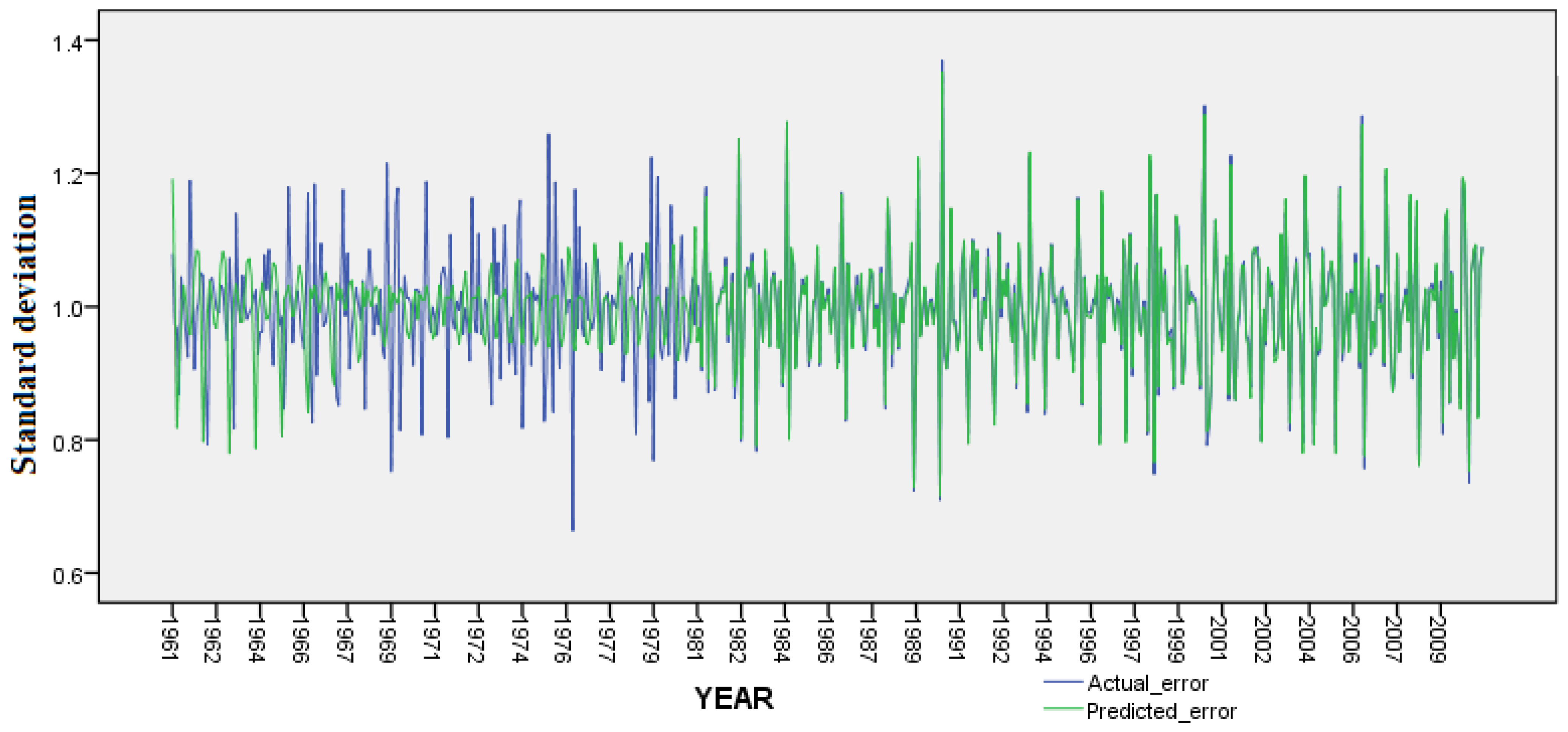
The standard deviation of the actual error and predicted error is calculated to know the error difference between the actual data set and the model selected for the forecast. It is evident in Figure 10 that the predicted error of the selected model is less than the actual data set; hence, the selected model is the best fit for the forecast.
The explanatory power R2 of the selected model shows that the model is capable of explaining 92.2% of the dataset for forecasting. Similarly, the value of RMSE as 25.2 and MAPE as 20.1 shows the prediction accuracy, and it also indicates the forecast error is less. Based on the data set scale, the value of MAPE and MAE as 20.1 and 14.1 indicates good tolerance. Table 1 illustrates the value of these parameters.
These results extrapolated the missing value, which can be used as a reference for further studies of the Kabul River. The linearity in the missing data makes sense as there were unknown factors involved that produced unknown water levels for the missing period. The forecast shows that provided the temperature and precipitation remain constant from the coming years, there will be no significant change in the water levels in the Kabul River. However, in case of weather shifts or anomalies, this forecast could still be useful as it could be used by the locals to earn a living above this water level to ensure safety in the future. It could also prove useful for the hydrologists, structural engineers, and flood disaster management officials to construct the water withholding structure with a capacity of these water levels.
To elaborate on the results further, this study predicts the data from 2011–2030. It can be seen that the trend of the past (1961–2010) is considerably different than the forecasted (2011–2030) trend. The reason is, firstly, the choice of considering the constant conditions in the future. The missing data could be linear or non-linear; however, for the analysis purposes, the analysis was performed using linear models as non-linearity could have greatly affected the results and might have deviated from the actual scenario of the river. Secondly, as the data were not collected by the concerned agencies till 2010 and there are no further official data available that could accurately forecast the water levels for the coming years, the data of the missing years have not been taken into account while conducting the analysis. To unravel the anomalies in the hydrologic behavior of the river, linear behavior was adopted to forecast the missing data closer to the previously recorded data.

5. Discussion

The analysis of missing years (2000–2020) was carried out as a forecast to help the hydrologists account for the missing data. To give an idea of the situation of the missing data of the year 2000–2020, it was estimated that water availability in 2015 was reduced to 1032 m3 from 5000 m3 in 1947 [82]. As Pakistan constructed the Warsak dam on the Kabul River, the decreased flow resulted in reduced water flow for the canal system, and the area irrigated by the Kabul canal system was reduced to 25,967 acres in 2015–2016 from 26,200 in 2015–2016 [83]. The glacier dynamics have had a significant impact on the water flow of the Kabul River. The 84% less snow that occurred from the year 2001–2016 shows that the solid precipitation will decrease with time, which will result in lower water flow in the Kabul River, which might lead the area to drought in the basin [84]. Two small dams were constructed in Afghanistan, namely, the Qargha and Band-i-Amir, with the help of US aid in 2008; if these dams become fully operational, it will have disastrous effects in terms of hydrogeneration and irrigation [85]. In 2003 and 2005, the Kabul Basin treaty between Pakistan and Afghanistan was drafted, but it failed miserably due to the unavailability of the water flow data [28]. Pakistan’s water supply from the Kabul River is hostage to the construction development and political stability in the Afghanistan region, and to the climatic conditions as any construction of the dam in Afghanistan region will result in a decrease of 25% less mean annual flow of Kabul River by the end of 2018 [86]. A study revealed that the increase of water demand and construction of more dams in Afghanistan will decrease its flow to 17% below the current flow of 8 million-acre-feet (MAF). This condition, along with climate variation, will give rise to a shortage of water in the Pakistan region [87,88].
To maximize the gross advantages of river management, a high-quality water inflow forecast is mandatory. This surface water is extremely important for the socio-economic development and growth of the region. Water infrastructure developments, floods, and droughts controlling industrial operations are all dependent upon this resource, thereby making efficient management of this resource necessary. Precise water flow prediction not only reduces the risks of mal-operation and probability of damages but also causes an increase in profits [89].
The stochastic nature of river flow makes its forecasting imperative for early hazard management. This forecasting of river water flow becomes even more vital in mountainous regions because a hefty-sized population living downstream is highly dependent upon this water resource for their agriculture and other economic activities [64]. There are early warning systems available, which, to manage water, produce an early measurement of water flow, but these warning systems are too expensive for poor communities to gain an advantage from them [90]; hence, the use of previous flood repetition data can be used to predict the future flood frequency, which could function as an early warning system regarding flood prediction. For this purpose, various contributing factors of the flood could be taken into account during analysis to help model water behavior. The findings of this study help to account for the missing data and forecast the data based on the weather of the data used for analysis. As the weather is unpredictable and is subject to change with the increase in global warming in the coming years, this study could prove to be a breakthrough in assessing the river behavior so that flood controlling devices are constructed with the required water-holding capacity. In recent times, artificial intelligence algorithms have been used by researchers to predict stream and river flow. As machine learning algorithms are based on statistical data, they generate highly accurate results and predictions. In this regard, Pianosi and Thi [91] estimated river water flow, and Wu and Han [92] estimated daily run-off in rivers using artificial intelligence algorithms. However, Agung [64] argues that care must be taken as the exact value of any parameter is never known; therefore, one should not rely on these models solely. He further maintains that a professional’s knowledge and experience should also be taken into account in defining several alternate models because in statistical analysis the best out of all options can never be achieved.
Based on the obtained results, the predictive performance of the selected model (2,4)(2,2) is evaluated statistically by the test data set of the decade 2000–2010 as done by Yu and Lei [69] in his research. The predicted results were up to par, with a few ambiguities where sharp fluctuations of water flow occurred. The model was selected based on AIC [65].
The subject river of the current study, the Kabul River, is the major tributary of the Indus River. Flooding in Kabul results in flooding in Indus as well. In 2010, the disastrous flood in Kabul and Sawat Rivers killed as many as 1156 people and affected 3.8 million people only in KP province [93]. Using past data to predict future water flow, hidden information can be disclosed that is of pronounced importance for alleviating the effects of floods and thwarting disasters. The generated best-fit model (2,4)(2,2) indicates the water flow to be 250 cumecs or a little above it in the next ten years. The result forecasted in the selected model is, therefore, highly beneficial for the river basin management where river flow, particularly in the rainy season, becomes a major challenge to handle. It provides compelling results to river management on how they can make maximum use of the study and fulfils the needs of the relevant stakeholders, although it should be kept in mind that even highly accurate water flow prediction does not always proliferate the benefits because ultimately it depends upon the operational strategies of the river administration [89].
This study can be generalized to other areas as the method employed in this study is automatic forecasting, which performs forecasting by identifying the best-suited model based on the lowest values of AIC. This tool selected ARMA (2,4)(2,2) based on the linear measurement of the past hydrological data. The significance of this work is that forecasted results can be a clarion call for the policymakers to allocate funding to the reservoir to work at its full capacity without damaging its structure, which will be beneficial for the agriculture sector, hydroelectric generation, and industrial processes and help designers and water management engineers to make sustainable decisions. From the civil engineering perspective, this study could help designers to complete sustainable basin designs, construct dams for electric generation, design canals for maximum agriculture productivity, and reconstruct and rehabilitate damaged water tributaries to meet flood and stormwater discharge, all of which could help save fertile land from being lost due to natural disasters like 2010 floods. If Pakistan completes hydroelectric projects in time, it can meet its electricity demands in the future. The outflow of this river depends on its basin condition, and the poor condition of this basin could lead to continuous silting in Warsak dam, the underperformance of hydropower generation, more frequent floods, less available water for agricultural needs, and inability of the river to meet the needs of the people relying on it. The construction of water storage structures and rehabilitation of the waterbed of the basin will ensure the likelihood of the people who are dependent for their survival on the Kabul River.
Despite using modern techniques for forecasting, there is always an uncertainty factor in the results; therefore, the quantification of climate is essential for the development of hydrologic impact. The uncertainty of results in this study is directly dependent on the precipitation and the temperature variation with each passing year. For improved modelling reliability, these two factors must be adequately addressed. As for this study, the forecasting accuracy will deviate from the actual water flow and its variation in precipitation and temperature change. For example, the temperature in 2010 was not the highest recorded temperature yet there were floods recorded in 2010 in Khyber Pakhtunkhwa province of Pakistan. Secondly, the precipitation was unexpectedly highest and there were no official early alarm systems. Provided the change in these two factors, the forecasted values of this study might prove inconsistent as this study did not account for the change in the precipitation and temperature change. Similarly, the absence of accurate data could seriously affect the observation uncertainty for floods and droughts as it could reveal the mean and variance of the streamflow in the Kabul Basin.
In recent years, the forecasting capability has increased significantly and has found its applications in all fields [86,87,88]. On the flip side, certain factors contribute towards many surprises in the analysis. Unfortunately, these factors can neither be modelled nor predicted; hence, the analysis is always accepted with a certain degree of uncertainty. Temperature, precipitation, and earthquakes are a few examples that could result in catastrophic loss of human life. Climate change is on the rise and is continuously wreaking havoc in the shape of tsunamis and hurricanes, which cannot be modelled. There might be damaging consequences if the forecast fails to accurately predict the water levels in the Kabul Basin. The inaccuracy could lead to extreme disasters like floods and droughts in the basin, which could threaten human existence. As Pakistan has constructed the Warsak dam on the Kabul River, which is regarded as one of the major dams of Pakistan, any fluctuation in the water level could create a power shortfall and the country would be plunged into the darkness.

6. Conclusions

Keeping in view the importance of the country’s major river in terms of the economy, hydroelectricity, and human existence, an analysis was undertaken to study and predict the water level from the year 2011 till the year 2030 based on historical trends. The Kabul River poses a threat to Pakistani soil in extreme conditions either by being flooded excessively due to the melting of glaciers and incessant precipitation or due to severe spells of droughts. Therefore, the need for forecasting is essential for the planning and management of future development. This development is based on forecasted values, and this study will not only serve the inhabitants of the country in extreme conditions but also will prove beneficial in energy generation. To prevent the devastation due to extreme water levels of the Kabul River, this study made necessary the use of the ML approach to forecast the water level so that engineers and decision-makers could apply preventive techniques to tackle extreme conditions. This research bridges the gap of missing data and connects it to the forecasted data. Based on the analysis of the hydrological data, the forecasting was evaluated by comparing it to the actual values, and it was found that ARMA (2,4)(2,2) accuracy was better than other modes based on the lowest values of AIC. The forecast revealed that the water level will not fluctuate much, the water level in Kabul River will be marginally more than 250 cumecs from 2011 till 2030, and there will be a diminutive difference in its quantity as compared to its value of 249 cumecs in 2000. It was also concluded that water level will gradually increase from January to August till it reaches its maximum level of 250 cumecs in September. As soon as the monsoon season diminishes, the water level will return to its minimum value of 10 cumecs in the months from October to December till the year 2030.

Author Contributions

M.A.M. conceptualization; data curation; formal analysis; investigation; methodology; writing—original draft; W.S.A. project administration; resources; supervision; writing—review & editing; M.B.A.R. investigation; software; writing—review & editing; M.A. (Mujahid Ali) data curation; validation; visualization; M.A. (Muhammad Altaf) conceptualization; data curation; formal analysis; methodology; R.F. funding acquisition; project administration; resources; N.V. funding acquisition; project administration; visualization; S.K. funding acquisition; project administration; supervision; H.B. methodology; validation; writing—original draft; A.S. data curation; formal analysis; methodology; W.R. data curation; investigation; methodology; W.F. data curation; writing—review & editing. All authors have read and agreed to the published version of the manuscript.

Funding

The research is partially funded by the Ministry of Science and Higher Education of the Russian Federation as part of World-class Research Center program: Advanced Digital Technologies (contract No. 075-15-2020-934 dated 17 November 2020).

Institutional Review Board Statement

Not applicable.

Informed Consent Statement

Not applicable.

Data Availability Statement

All the data is available within this manuscript.

Acknowledgments

The authors would like to thank Universiti Teknologi PETRONAS (UTP) for the support provided for this research.

Conflicts of Interest

The authors declare no conflict of interest.

Abbreviations

GDPGross Domestic Product
MLMachine Learning
ANNArtificial Neural Network
AN-FISAdaptive Neuro-Fuzzy Inference Systems
ARAutoregressive
MAMoving Average
ARMAAutoregressive Moving Average
MAEMean Absolute Error
MSEMean Squared Error
SVMSupport Vector Machine
LSSVMLeast-Squares SVM
GRNNGeneralized Regression Neural Networks
WANNWavelet-Based Artificial Neural Network
WANFISWavelet-Based Adaptive Neuro-Fuzzy Inference System
RMSERoot Mean Squared Error
MAPEMean Absolute Percent Error
ARIMAAutoregressive Integrated Moving Average
ADFAugmented Dickey Fuller
AICAkaike Information Criteria
BICBayesian Information Criteria
KPKhyber Pakhtunkhwa
WAPDAWater and Power Development Authority
HQHannan-Quinn Criterion
Residual ACFResidual Autocorrelation Function
Residual PACFResidual Partial Autocorrelation Function
CIConfidence Interval
MAFMillion Acre-Feet

Appendix A

Table A1. Model Selection Criteria.
S.NoModelLogLAIC *BICHQ
1(2,4)(2,2)−2199.739.2155389.3198839.256554
2(1,0)(2,2)−2205.259.2177299.2785979.241655
3(2,0)(2,2)−2205.089.2211579.290729.248501
4(1,1)(2,2)−2205.099.2212059.2907689.248549
5(4,3)(2,2)−2200.179.2215579.3345979.265991
6(2,4)(1,2)−2202.269.2219059.3175559.259503
7(1,0)(2,1)−2207.469.2227639.2749359.243271
8(1,0)(1,2)−2207.529.2229849.2751569.243492
9(2,1)(2,2)−2204.939.2247069.3029649.255468
10(0,2)(2,2)−22069.2249919.2945549.252335
11(3,0)(2,2)−2205.029.2250849.3033439.255846
12(1,2)(2,2)−2205.049.2251629.303429.255924
13(0,3)(2,2)−2205.079.2252919.303559.256053
14(3,4)(2,1)−2202.289.2261499.3304949.267165
15(2,0)(2,1)−2207.379.2265599.2874269.250484
16(1,1)(2,1)−2207.389.2265849.2874529.25051
17(2,0)(1,2)−2207.439.2267719.2876399.250697
18(1,1)(1,2)−2207.439.2267989.2876659.250723
19(1,0)(1,1)−2209.799.2283039.271789.245392
20(2,2)(2,2)−2204.939.2288729.3158269.263052
21(3,1)(2,2)−2204.939.2288729.3158269.263052
22(4,0)(2,2)−2204.989.2290929.3160469.263271
23(0,4)(2,2)−22059.229179.3161239.263349
24(1,3)(2,2)−2205.019.229219.3161649.26339
25(0,2)(2,1)−2208.179.2298829.290759.253808
26(0,2)(1,2)−2208.239.2301119.2909789.254036
27(2,1)(2,1)−2207.259.2302129.2997759.257556
28(2,1)(1,2)−2207.299.2303639.2999279.257707
29(3,0)(2,1)−2207.319.2304669.3000299.25781
30(1,2)(2,1)−2207.339.2305289.3000919.257872
31(3,0)(1,2)−2207.369.2306789.3002419.258022
32(0,3)(2,1)−2207.379.2306939.3002569.258037
33(1,2)(1,2)−2207.389.230749.3003039.258084
34(0,3)(1,2)−2207.429.2309039.3004669.258246
35(2,0)(1,1)−2209.579.2315579.283739.252065
36(1,1)(1,1)−2209.599.2316079.2837799.252114
37(3,2)(2,2)−2204.849.232659.32839.270248
38(2,3)(2,2)−2204.929.2329959.3286449.270593
39(4,1)(2,2)−2204.929.2330059.3286559.270603
40(1,4)(2,2)−22059.2333359.3289849.270933
41(4,4)(1,1)−2204.059.2335359.337889.274551
42(3,1)(2,1)−2207.239.2342769.3125359.265038
43(2,2)(2,1)−2207.249.2343339.3125929.265095
44(2,2)(1,2)−2207.289.23459.3127589.265262
45(3,1)(1,2)−2207.289.2345019.312769.265263
46(4,0)(2,1)−2207.289.2345159.3127739.265277
47(0,4)(2,1)−2207.39.2345689.3128269.26533
48(1,3)(2,1)−2207.339.2346919.3129499.265452
49(4,0)(1,2)−2207.339.2347269.3129849.265488
50(0,4)(1,2)−2207.359.234789.3130389.265542
51(1,3)(1,2)−2207.369.2348269.3130859.265588
52(0,2)(1,1)−2210.49.2350099.2871819.255517
53(2,1)(1,1)−2209.479.2353049.2961729.25923
54(3,0)(1,1)−2209.549.2355669.2964349.259492
55(1,2)(1,1)−2209.559.2356299.2964979.259555
56(0,3)(1,1)−2209.589.2357459.2966139.259671
57(4,2)(2,2)−2204.829.2367639.3411089.277779
58(3,3)(2,2)−2204.829.2367649.3411089.277779
59(4,1)(1,2)−2207.149.2380989.3250529.272277
60(3,2)(1,2)−2207.159.2381299.3250839.272309
61(2,3)(2,1)−2207.229.2384119.3253659.272591
62(3,2)(2,1)−2207.239.2384719.3254259.272651
63(4,1)(2,1)−2207.39.238739.3256849.272909
64(1,4)(2,1)−2207.39.2387339.3256879.272913
65(1,4)(1,2)−2207.359.2389459.3258989.273124
66(2,3)(1,2)−2207.379.2390319.3259859.273211
67(2,2)(1,1)−2209.479.2394719.3090349.266814
68(3,1)(1,1)−2209.479.2394719.3090349.266815
69(4,0)(1,1)−2209.59.2395839.3091469.266927
70(0,4)(1,1)−2209.529.2396529.3092159.266996
71(1,3)(1,1)−2209.539.2396939.3092569.267037
72(3,4)(2,2)−2204.829.2409299.3539699.285363
73(4,3)(1,1)−2206.939.241399.337049.278988
74(4,2)(2,1)−2207.059.2418569.3375059.279454
75(3,3)(2,1)−2207.059.2418649.3375139.279462
76(4,2)(1,2)−2207.19.2420979.3377469.279694
77(3,3)(1,2)−2207.199.2424719.338129.280069
78(2,4)(2,1)−2207.289.2428499.3384989.280447
79(3,2)(1,1)−2209.49.2433289.3215869.274089
80(2,3)(1,1)−2209.459.243549.3217999.274302
81(1,4)(1,1)−2209.529.2438189.3220779.274580
82(4,1)(1,1)−2209.529.2438329.322099.274593
83(4,4)(2,2)−2204.829.2451039.3668399.292955
84(3,4)(1,2)−2207.19.246259.3505949.287265
85(4,3)(2,1)−2207.239.2467899.3511349.287805
86(4,3)(1,2)−2207.299.2470219.3513669.288037
87(3,3)(1,1)−2209.469.2477559.3347089.281934
88(4,2)(1,1)−2209.469.2477649.3347189.281943
89(2,4)(1,1)−2209.519.2479739.3349279.282152
90(0,1)(2,2)−2212.549.2480829.308959.272008
91(4,4)(2,1)−2207.219.2508969.3639369.295329
92(4,4)(1,2)−2207.279.2511369.3641769.295569
93(0,1)(2,1)−2214.379.2515359.3037089.272043
94(0,1)(1,2)−2214.449.2518279.3039999.272335
95(3,4)(1,1)−2209.459.2518729.3475229.28947
96(0,1)(1,1)−2216.449.2560119.2994889.273101
97(4,4)(2,0)−2243.039.3959719.5003159.436986
98(3,2)(2,0)−2248.999.4083059.4865649.439067
99(4,2)(2,0)−2248.499.4103929.4973469.444572
100(3,3)(2,0)−2248.519.4104419.4973959.444621
101(3,4)(2,0)−2248.859.416039.5116799.453628
102(0,0)(2,1)−2256.929.4246829.4681599.441771
103(2,1)(2,0)−2254.989.4249159.4857839.448841
104(0,0)(1,2)−2257.029.4250759.4685529.442165
105(0,0)(2,2)−2256.499.4270519.4792239.447558
106(2,2)(2,0)−2254.919.4287859.4983489.456128
107(3,1)(2,0)−2254.919.4288119.4983749.456154
108(2,3)(2,0)−2254.829.4325859.5108449.463347
109(4,1)(2,0)−2254.829.4325989.5108569.46336
110(0,0)(1,1)−2261.79.4404259.4752069.454097
111(1,0)(2,0)−2261.249.4426839.486169.459773
112(4,3)(2,0)−2256.179.4465329.5421819.484129
113(2,0)(2,0)−2261.219.4467279.4988999.467235
114(1,1)(2,0)−2261.229.4467319.4989049.467239
115(3,0)(2,0)−2261.29.4508289.5116969.474754
116(1,2)(2,0)−2261.219.450869.5117289.474786
117(0,3)(2,0)−2261.249.450989.5118489.474906
118(0,2)(2,0)−2262.259.4510279.5031999.471535
119(4,0)(2,0)−2261.059.454369.5239239.481704
120(0,4)(2,0)−2261.099.4545629.5241269.481906
121(1,3)(2,0)−2261.149.4547439.5243069.482087
122(2,4)(2,0)−2259.239.4551259.5420799.489304
123(1,4)(2,0)−2261.099.458719.5369689.489471
124(0,1)(2,0)−2267.539.4688669.5123439.485956
125(4,4)(0,0)−2276.039.5251389.6120929.559318
126(4,2)(1,0)−2285.39.5596019.637869.590363
127(3,3)(1,0)−2285.549.5605999.6388589.591361
128(3,4)(1,0)−2285.419.5641989.6511529.598378
129(4,3)(1,0)−2287.739.5738579.6608119.608036
130(4,4)(1,0)−2287.699.5778829.6735329.61548
131(2,2)(1,0)−2294.689.5903379.6512059.614263
132(3,1)(1,0)−2294.719.5904759.6513439.614401
133(3,2)(1,0)−2294.629.5942459.6638089.621589
134(2,3)(1,0)−2294.659.5943739.6639369.621716
135(4,1)(1,0)−2294.679.5944579.664029.621801
136(2,4)(1,0)−2299.799.6199789.6982379.65074
137(1,0)(1,0)−2305.149.621429.6562019.635091
138(2,0)(1,0)−2305.139.6255549.6690319.642644
139(1,1)(1,0)−2305.139.6255589.6690359.642648
140(3,0)(1,0)−2304.879.6286149.6807869.649122
141(0,3)(1,0)−2304.919.6288069.6809789.649314
142(1,2)(1,0)−2304.949.6289239.6810959.649431
143(0,0)(2,0)−2307.029.6292489.6640299.64292
144(0,2)(1,0)−2306.029.6292649.6727419.646354
145(2,1)(1,0)−2305.099.6295539.6817259.65006
146(4,0)(1,0)−2304.549.6314269.6922939.655352
147(0,4)(1,0)−2304.89.6325089.6933769.656434
148(1,3)(1,0)−2304.859.6326969.6935649.656622
149(1,4)(1,0)−2304.789.6365639.7061269.663907
150(0,1)(1,0)−2312.919.6537959.6885779.667467
151(4,3)(0,2)−2308.279.6636269.7592759.701224
152(4,2)(0,1)−2316.499.689549.7677989.720301
153(3,4)(0,2)−2316.039.6959699.7916199.733567
154(4,3)(0,1)−2317.819.6991939.7861479.733372
155(2,4)(0,2)−2319.559.7064529.7934069.740632
156(4,2)(0,0)−2338.739.7780569.8476199.8054
157(4,3)(0,0)−2342.369.7973239.8755819.828085
158(0,0)(1,0)−23509.8041619.8302479.814415
159(2,3)(0,1)−2354.759.8448099.9143729.872153
160(3,4)(0,1)−2355.369.8556649.9426189.889844
161(4,4)(0,2)−2362.949.8955849.9999299.9366
162(3,2)(0,2)−2366.889.8995029.9777619.930264
163(2,1)(0,2)−2369.399.9016289.9624969.925554
164(2,2)(0,2)−2368.579.9023629.9719259.929706
165(3,1)(0,2)−2368.669.9027329.9722959.930076
166(3,3)(0,2)−2366.749.9030849.9900389.937264
167(4,2)(0,2)−2366.759.9031149.9900679.937293
168(4,1)(0,2)−2368.049.9043459.9826039.935106
169(4,0)(0,2)−2386.589.97741410.0469810.00476
170(1,4)(0,2)−2385.589.97741910.0556810.00818
171(3,0)(0,2)−2389.539.98554810.0464210.00947
172(4,4)(0,1)−2386.69.99000110.0856510.0276
173(4,1)(0,1)−2396.3910.018310.0878710.04565
174(2,4)(0,0)−2396.7210.0196510.0892210.047
175(2,2)(0,1)−2397.9310.0205410.081410.04446
176(3,1)(0,1)−2398.2910.0220610.0829310.04599
177(2,0)(0,2)−2399.6610.0235610.0757410.04407
178(3,3)(0,1)−2396.8610.0244210.1026810.05518
179(2,1)(0,1)−2400.3910.0266110.0787810.04712
180(1,3)(0,2)−2401.7810.0407710.1103310.06811
181(0,3)(0,2)−2404.0710.0461310.1069910.07005
182(0,4)(0,2)−2403.7110.048810.1183610.07614
183(1,2)(0,2)−2405.9810.054110.1149710.07803
184(3,3)(0,0)−2410.1210.075510.1450710.10285
185(0,2)(0,2)−2413.0910.0795610.1317310.10007
186(1,1)(0,2)−2415.1310.0880610.1402310.10857
187(3,4)(0,0)−2414.3310.097210.1754610.12797
188(2,4)(0,1)−2420.8610.1244110.2026610.15517
189(4,0)(0,1)−2425.710.1362510.1971210.16018
190(1,4)(0,1)−2425.0310.1376310.2071910.16497
191(3,0)(0,1)−2428.2810.1428310.1950110.16334
192(1,0)(0,2)−2432.8510.157710.2011810.17479
193(2,0)(0,1)−2438.0210.1792710.2227510.19636
194(2,3)(0,2)−2443.5510.2189410.297210.24970
195(4,1)(0,0)−2446.5710.223210.2840710.24713
196(0,3)(0,1)−244810.2250210.2771910.24553
197(0,4)(0,1)−2447.5310.2272310.288110.25115
198(0,1)(0,2)−2451.8110.2367210.2801910.25381
199(1,3)(0,1)−2450.4710.2394710.3003410.26340
200(2,2)(0,0)−2457.9910.2666210.3187910.28713
* Indicates the preferred parameter for the selection of ARIMA model in this study.

Appendix B

Figure A1. Automated ARIMA parameters.
Sustainability 13 10720 g0a1

Appendix C

Figure A2. Model Validation Features.
Sustainability 13 10720 g0a2

References

  1. Haidvogl, G. Historic milestones of human river uses and ecological impacts. In Riverine Ecosystem Management; Huisman, J., Ed.; Springer: Berlin/Heidelberg, Germany, 2018; pp. 19–39. [Google Scholar]
  2. Aslam, B.; Maqsoom, A.; Alaloul, W.S.; Musarat, M.A.; Jabbar, T.; Zafar, A. Soil erosion susceptibility mapping using a GIS-based multi-criteria decision approach: Case of district Chitral, Pakistan. Ain Shams Eng. J. 2021, 12, 1637–1649. [Google Scholar] [CrossRef]
  3. Ahmed, I.; Debnath, J.; Das, N. Impact of river on human life: A case study on the Gumti River, Tripura. Radix International. J. Res. Soc. Sci. 2015, 4, 1–13. [Google Scholar]
  4. Zhang, Y.; Xia, J.; Liang, T.; Shao, Q. Impact of Water Projects on River Flow Regimes and Water Quality in Huai River Basin. Water Resour. Manag. 2009, 24, 889–908. [Google Scholar] [CrossRef]
  5. Nguyen, X.H. Combining statistical machine learning models with ARIMA for water level forecasting: The case of the Red river. Adv. Water Resour. 2020, 142, 103656. [Google Scholar]
  6. Sapitang, M.; Ridwan, W.M.; Kushiar, K.F.; Ahmed, A.N.; El-Shafie, A. Machine Learning Application in Reservoir Water Level Forecasting for Sustainable Hydropower Generation Strategy. Sustainability 2020, 12, 6121. [Google Scholar] [CrossRef]
  7. Khatibi, R.; Sivakumar, B.; Ghorbani, M.A.; Kisi, O.; Koçak, K.; Zadeh, D.F. Investigating chaos in river stage and discharge time series. J. Hydrol. 2012, 414, 108–117. [Google Scholar] [CrossRef]
  8. Mack, T.J.; Chornack, M.P.; Taher, M.R. Groundwater-level trends and implications for sustainable water use in the Kabul Basin, Afghanistan. Environ. Syst. Decis. 2013, 33, 457–467. [Google Scholar] [CrossRef] [Green Version]
  9. Iqbal, M.S.; Hofstra, N. Modeling Escherichia coli fate and transport in the Kabul River Basin using SWAT. Hum. Ecol. Risk Assess. Int. J. 2018, 25, 1279–1297. [Google Scholar] [CrossRef] [Green Version]
  10. Mehmood, A.; Jia, S.; Lv, A.; Zhu, W.; Mahmood, R.; Saifullah, M.; Adnan, R. Detection of Spatial Shift in Flood Regime of the Kabul River Basin in Pakistan, Causes, Challenges, and Opportunities. Water 2021, 13, 1276. [Google Scholar] [CrossRef]
  11. Khan, H.F.; Yang, Y.C.E.; Wi, S. Case Study on Hydropolitics in Afghanistan and Pakistan: Energy and Water Impacts of Kunar River Development. J. Water Resour. Plan. Manag. 2020, 146, 05020015. [Google Scholar] [CrossRef]
  12. Qureshi, W.A. Water as a human right: A case study of the Pakistan-India water conflict. Penn St. JL Int’l Aff. 2017, 5, 374. [Google Scholar]
  13. Tariq, M.A.; van de Giesen, N.; Janjua, S.; Shahid, M.L.; Farooq, R. An engineering perspective of water sharing issues in Pakistan. Water. 2020, 12, 477. [Google Scholar] [CrossRef] [Green Version]
  14. Ghulami, M.; Gourbesville, P.; Audra, P. Assessing Future Water Availability Under a Changing Climate in Kabul Basin. Adv. Hydroinform. 2020, 1, 647–657. [Google Scholar]
  15. Haider, R. Climate Change Projections of Kabul River Basin using Multi-Model Ensemble. Leadersh. Environ. Dev. Pak. 2018, 2, 1–4. [Google Scholar]
  16. Chaudhry, Q.U.Z. Climate Change Profile of Pakistan; Asian Development Bank: Mandaluyong, Philippines, 2017; pp. 1–130. [Google Scholar]
  17. Sayama, T.; Ozawa, G.; Kawakami, T.; Nabesaka, S.; Fukami, K. Rainfall–runoff–inundation analysis of the 2010 Pakistan flood in the Kabul River basin. Hydrol. Sci. J. 2012, 57, 298–312. [Google Scholar] [CrossRef]
  18. Hanasz, P. The politics of water security in the Kabul river basin. Atl. Mon. 2011, 10, 1–7. [Google Scholar]
  19. Rasul, G.; Chaudhry, Q.Z.; Mahmood, A.; Hyder, K.W.; Dahe, Q. Glaciers and glacial lakes under changing climate in Pakistan. Pak. J. Meteorol. 2011, 8, 1–8. [Google Scholar]
  20. Nafees, M. Role of Kabul River in Socio-economic Activities and Associated Environmental Problems. Cent. Asia 2010, 67, 83–97. [Google Scholar]
  21. Nafees, M.; Shabir, A.; Zahid, U. Construction of dam on Kabul River and its socio-economic implication for Khyber Pukhtunkhwa, Pakistan. Semin. Pak.–Afghan Water Shar. Issue 2016, 23, 2016. [Google Scholar]
  22. Pakistan. Government of Warsak Hydroelectric Power Station 2nd Rehabilitation Project. 2015. Available online: https://mowr.gov.pk/index.php/warsak-hydroelectric-power-station-2nd-rehabilitation-project/ (accessed on 12 April 2021).
  23. Iqbal, M.S.; Dahri, Z.H.; Querner, E.P.; Khan, A.; Hofstra, N. Impact of Climate Change on Flood Frequency and Intensity in the Kabul River Basin. Geoscience 2018, 8, 114. [Google Scholar] [CrossRef] [Green Version]
  24. Hasson, S.U.; Saeed, F.; Böhner, J.; Schleussner, C.-F. Water availability in Pakistan from Hindukush–Karakoram–Himalayan watersheds at 1.5 °C and 2 °C Paris Agreement targets. Adv. Water Resour. 2019, 131, 103365. [Google Scholar] [CrossRef]
  25. Britannica, T.E.O.E. Pakistan Floods of 2010; Tesch, N., Ed.; Encyclopedia Britannica Press; Britannica, UK, 2020. [Google Scholar]
  26. O’Neill, A. Pakistan: Distribution of Employment by Economic Sector from 2010 to 2020. Available online: statista.com (accessed on 11 April 2021).
  27. Taraky, Y.; Liu, Y.; McBean, E.; Daggupati, P.; Gharabaghi, B. Flood Risk Management with Transboundary Conflict and Cooperation Dynamics in the Kabul River Basin. Water 2021, 13, 1513. [Google Scholar] [CrossRef]
  28. Khattak, M.S.; Anwar, F.; Saeed, T.U.; Sharif, M.; Sheraz, K.; Ahmed, A. Floodplain Mapping Using HEC-RAS and ArcGIS: A Case Study of Kabul River. Arab. J. Sci. Eng. 2015, 41, 1375–1390. [Google Scholar] [CrossRef]
  29. Terzi, Ö.; Ergin, G. Forecasting of monthly river flow with autoregressive modeling and data-driven techniques. Neural Comput. Appl. 2014, 25, 179–188. [Google Scholar] [CrossRef]
  30. Yaseen, Z.M.; El-Shafie, A.; Jaafar, O.; Afan, H.A.; Sayl, K.N. Artificial intelligence based models for stream-flow forecasting: 2000–2015. J. Hydrol. 2015, 530, 829–844. [Google Scholar] [CrossRef]
  31. Mohammed, M.; Khan, M.B.; Bashier, E.B.M. Machine Learning: Algorithms and Applications; CRC Press: Boca Raton, FL, USA, 2016. [Google Scholar]
  32. Mullainathan, S.; Spiess, J. Machine Learning: An Applied Econometric Approach. J. Econ. Perspect. 2017, 31, 87–106. [Google Scholar] [CrossRef] [Green Version]
  33. Zakaria, M.N.A.; Malek, M.A.; Zolkepli, M.; Ahmed, A.N. Application of artificial intelligence algorithms for hourly river level forecast: A case study of Muda River, Malaysia. Alex. Eng. J. 2021, 60, 4015–4028. [Google Scholar] [CrossRef]
  34. Piri, J.; Kahkha, M.R.R. Prediction of water level fluctuations of Chahnimeh reservoirs in Zabol using ANN, ANFIS and cuckoo optimization algorithm. Iran. J. Health Saf. Environ. 2017, 4, 706–715. [Google Scholar]
  35. Üneş, F.; Demirci, M.; Tasar, B.; Kaya, Y.Z.; Varcin, H. Estimating dam reservoir level fluctuations using data-driven techniques. Pol. J. Environ. Stud. 2019, 28, 3451–3462. [Google Scholar] [CrossRef]
  36. Seo, Y.; Kim, S.; Singh, V.P. Multistep-ahead flood forecasting using wavelet and data-driven methods. KSCE J. Civ. Eng. 2015, 19, 401–417. [Google Scholar] [CrossRef]
  37. Seo, Y.; Kim, S.; Kisi, O.; Singh, V.P. Daily water level forecasting using wavelet decomposition and artificial intelligence techniques. J. Hydrol. 2015, 520, 224–243. [Google Scholar] [CrossRef]
  38. Guo, T.; He, W.; Jiang, Z.; Chu, X.; Malekian, R.; Li, Z. An Improved LSSVM Model for Intelligent Prediction of the Daily Water Level. Energies 2018, 12, 112. [Google Scholar] [CrossRef] [Green Version]
  39. Jamil, R. Hydroelectricity consumption forecast for Pakistan using ARIMA modeling and supply-demand analysis for the year 2030. Renew. Energy 2020, 154, 1–10. [Google Scholar] [CrossRef]
  40. Dickey, D.A.; Fuller, W.A. Distribution of the estimators for autoregressive time series with a unit root. J. Am. Stat. Assoc. 1979, 74, 427–431. [Google Scholar]
  41. Fuller, W.A. Introduction to Statistical Time Series; John Wiley & Sons: Hoboken, NJ, USA, 1976. [Google Scholar]
  42. Masani, R. Norbert Wiener 1894–1964; Birkhäuser: Basel, Switzerland, 2012; Volume 5. [Google Scholar]
  43. Box, G. Time Series Analysis: Forecasting and Control by George EP Box and Gwilym M; Holden-Day: San Francisco, CA, USA, 1970. [Google Scholar]
  44. Shahwan, T.; Odening, M. Forecasting agricultural commodity prices using hybrid neural networks. In Computational Intelligence in Economics and Finance; Springer: Berlin/Heidelberg, Germany, 2007; pp. 63–74. [Google Scholar]
  45. Whittle. Hypothesis Testing in Time Series Analysis; Almqvist & Wiksells boktr: Stockholm, Sweden, 1951; Volume 4. [Google Scholar]
  46. Hyndman, R.J.; Athanasopoulos, G. Forecasting: Principles and Practice, 2nd ed.; OTexts: Melbourne, Australia, 2018; Volume 1, pp. 1–384. [Google Scholar]
  47. Akaike, H. Information Theory and an Extension of the Maximum Likelihood Principle, in Selected Papers of Hirotugu Akaike; Springer: Berlin/Heidelberg, Germany, 1998; pp. 199–213. [Google Scholar]
  48. Hirotugu Akaike. Factor Analysis and AIC; Selected papers of Hirotugu Akaike; Springer: New York, NY, USA, 1987; pp. 371–386. [Google Scholar]
  49. Taddy, M. Business data science: Combining machine learning and economics to optimize, automate, and accelerate business decisions. McGraw Hill Prof. 2019, 1, 1–359. [Google Scholar]
  50. Akaike, H. A new look at the statistical model identification. IEEE Trans. Autom. Control 1974, 19, 716–723. [Google Scholar] [CrossRef]
  51. Schwarz, G. The annals of statistics. Estim. Dimens. A Model 1978, 6, 461–464. [Google Scholar]
  52. Burnham, K.P.; Anderson, D.R. A practical information-theoretic approach. Model Sel. Multimodel Inference 2002, 2, 267–344. [Google Scholar]
  53. Wit, E.; Heuvel, E.V.D.; Romeijn, J.W. ‘All models are wrong...’: An introduction to model uncertainty. Stat. Neerl. 2012, 66, 217–236. [Google Scholar] [CrossRef] [Green Version]
  54. Vrieze, S.I. Model selection and psychological theory: A discussion of the differences between the Akaike information criterion (AIC) and the Bayesian information criterion (BIC). Psychol. Methods 2012, 17, 228. [Google Scholar] [CrossRef] [Green Version]
  55. Burnham, K.P.; Anderson, D.R. Multimodel inference: Understanding AIC and BIC in model selection. Sociol. Methods Res. 2004, 33, 261–304. [Google Scholar] [CrossRef]
  56. Aho, K.; Derryberry, D.; Peterson, T. Model selection for ecologists: The worldviews of AIC and BIC. Ecology 2014, 95, 631–636. [Google Scholar] [CrossRef] [PubMed]
  57. Barnston, A.G. Correspondence among the correlation, RMSE, and Heidke forecast verification measures; refinement of the Heidke score. Weather. Forecast. 1992, 7, 699–709. [Google Scholar] [CrossRef] [Green Version]
  58. Kenney, J.F. Mathematics of Statistics; D. Van Nostrand: New York, NY, USA, 1939. [Google Scholar]
  59. Everitt, B.; Skrondal, A. The Cambridge Dictionary of Statistics; Cambridge University Press: Cambridge, UK, 2002; Volume 106. [Google Scholar]
  60. Read, C.B.; Vidakovic, B. Encyclopedia of Statistical Sciences; John Wiley & Sons: Hoboken, NJ, USA, 2006; Volume 2. [Google Scholar]
  61. Willmott, C.; Matsuura, K. Advantages of the mean absolute error (MAE) over the root mean square error (RMSE) in assessing average model performance. Clim. Res. 2005, 30, 79–82. [Google Scholar] [CrossRef]
  62. Dodge, Y. The Concise Encyclopedia of Statistics; Springer Science & Business Media: Berlin/Heidelberg, Germany, 2008. [Google Scholar]
  63. Khair, U.; Fahmi, H.; Al Hakim, S.; Rahim, R. Forecasting error calculation with mean absolute deviation and mean absolute percentage error. J. Phys. 2017, 930, 012002. [Google Scholar] [CrossRef]
  64. Agung, I.G.N. Time Series Data Analysis Using EViews; John Wiley & Sons: Hoboken, NJ, USA, 2011. [Google Scholar]
  65. Katimon, A.; Shahid, S.; Mohsenipour, M. Modeling water quality and hydrological variables using ARIMA: A case study of Johor River, Malaysia. Sustain. Water Resour. Manag. 2017, 4, 991–998. [Google Scholar] [CrossRef]
  66. Birylo, M.; Rzepecka, Z.; Kuczynska-Siehien, J.; Nastula, J. Analysis of water budget prediction accuracy using ARIMA models. Water Supply 2017, 18, 819–830. [Google Scholar] [CrossRef]
  67. Valipour, M.; Banihabib, M.E.; Behbahani, S.M.R. Comparison of the ARMA, ARIMA, and the autoregressive artificial neural network models in forecasting the monthly inflow of Dez dam reservoir. J. Hydrol. 2012, 476, 433–441. [Google Scholar] [CrossRef]
  68. Woodward, W.A.; Gray, H.L.; Elliott, A.C. Applied Time Series Analysis with R; CRC Press: Boca Raton, FL, USA, 2017. [Google Scholar]
  69. Yu, Z.; Lei, G.; Jiang, Z.; Liu, F. ARIMA modelling and forecasting of water level in the middle reach of the Yangtze River in 2017. In Proceedings of the 4th International Conference on Transportation Information and Safety (ICTIS), Banff, AB, Canada, 8–10 August 2017. [Google Scholar]
  70. Gao, Y.; Merz, C.; Lischeid, G.; Schneider, M. A review on missing hydrological data processing. Environ. Earth Sci. 2018, 77, 47. [Google Scholar] [CrossRef]
  71. Gao, Y. Dealing with missing data in hydrology: Data Analysis of Discharge and Groundwater Time-Series in Northeast Germany. Ph.D. Thesis, Freie Universität Berlin, Berlin, Germany, 2017. [Google Scholar]
  72. Gibrilla, A.; Anornu, G.; Adomako, D. Trend analysis and ARIMA modelling of recent groundwater levels in the White Volta River basin of Ghana. Groundw. Sustain. Dev. 2018, 6, 150–163. [Google Scholar] [CrossRef]
  73. Valipour, M. Long-term runoff study using SARIMA and ARIMA models in the United States. Meteorol. Appl. 2015, 22, 592–598. [Google Scholar] [CrossRef]
  74. Nigam, R.; Nigam, S.; Mittal, S.K. The river runoff forecast based on the modeling of time series. Russ. Meteorol. Hydrol. 2014, 39, 750–761. [Google Scholar] [CrossRef]
  75. Ghimire, B.N. Application of ARIMA Model for River Discharges Analysis. J. Nepal Phys. Soc. 2017, 4, 27–32. [Google Scholar] [CrossRef] [Green Version]
  76. Bin Shaari, M.A.; Samsudin, R.; Bin Shabri Ilman, A. Comparison of drought forecasting using ARIMA and empirical wavelet Transform-ARIMA. In Proceedings of the International Conference of Reliable Information and Communication Technology, Johor, Malaysia, 23–24 April 2017. [Google Scholar]
  77. Bazrafshan, O.; Salajegheh, A.; Bazrafshan, J.; Mahdavi, M.; Maraj, A.F. Hydrological drought forecasting using ARIMA models (case study: Karkheh Basin). Ecopersia 2015, 3, 1099–1117. [Google Scholar]
  78. Gharde, K.; Kothari, M.; Mahale, D. Developed seasonal ARIMA model to forecast streamflow for Savitri Basin in Konkan Region of Maharshtra on daily basis. J. Indian Soc. Coast. Agric. Res. 2016, 34, 110–119. [Google Scholar]
  79. Myronidis, D.; Ioannou, K.; Fotakis, D.; Dörflinger, G. Streamflow and Hydrological Drought Trend Analysis and Forecasting in Cyprus. Water Resour. Manag. 2018, 32, 1759–1776. [Google Scholar] [CrossRef]
  80. Rahaman, M.; Thakur, B.; Kalra, A.; Ahmad, S. Modeling of GRACE-Derived Groundwater Information in the Colorado River Basin. Hydrology 2019, 6, 19. [Google Scholar] [CrossRef] [Green Version]
  81. Guide, E.U. Automatic ARIMA Forecasting. 2020. Available online: http://www.eviews.com/help/helpintro.html#page/content%2Fseries-Automatic_ARIMA_Forecasting.html%23ww154388 (accessed on 20 April 2021).
  82. Azam, S. Kabul River Treaty: A Necessity for Peace-n-Security between Afghanistan and Pakistan, and Peace in South Asia. Gomal Univ. J. Res. 2015, 31, 134–145. [Google Scholar]
  83. Malik, T. Pak-Afghan Water Issue: A Case for Benefit-Sharing. Policy Perspect. 2019, 16, 77–98. [Google Scholar] [CrossRef]
  84. Masood, A.; Hashmi, M.Z.U.R.; Mushtaq, H. Spatio-Temporal Analysis of Early Twenty-First Century Areal Changes in the Kabul River Basin Cryosphere. Earth Syst. Environ. 2018, 2, 563–571. [Google Scholar] [CrossRef]
  85. Sultan, M.; Assadullah, A. New hydrological station at Qargha Dam to help manage Afghanistan’s water resources. Food Agric. Organ. 2008. Available online: https://reliefweb.int/report/afghanistan/new-hydrological-station-qargha-dam-help-manage-afghanistans-water-resources (accessed on 18 April 2021).
  86. Akhtar, S.M.; Iqbal, J. Assessment of emerging hydrological, water quality issues and policy discussion on water sharing of transboundary Kabul River. Hydrol. Res. 2017, 19, 650–672. [Google Scholar] [CrossRef] [Green Version]
  87. Atef, S.S.; Sadeqinazhad, F.; Farjaad, F.; Amatya, D.M. Water conflict management and cooperation between Afghanistan and Pakistan. J. Hydrol. 2019, 570, 875–892. [Google Scholar] [CrossRef]
  88. Khan, S.; Pervaz, I. The Brewing Conflict over Kabul River; Policy Options for Legal Framework. ISSRA Pap. 2014, 1, 17–38. [Google Scholar]
  89. Dong, X.; Dhmen-Janssen, C.M.; Booij, M.J.; Hulscher, S.J.M.H. Requirements and benefits of flow forecasting for improving hydropower generation. In Stochastic Hydraulics; IAHR: Madrid, Spain, 2005; pp. 60–63. [Google Scholar]
  90. Krajewski, W.F.; Ceynar, D.; Demir, I.; Goska, R.; Kruger, A.; Langel, C.; Mantilla, R.; Niemeier, J.; Quintero, F.; Seo, B.-C.; et al. Real-Time Flood Forecasting and Information System for the State of Iowa. Bull. Am. Meteorol. Soc. 2017, 98, 539–554. [Google Scholar] [CrossRef]
  91. Pianosi, F.; Thi, X.Q.; Soncini-Sessa, R. Artificial Neural Networks and Multi Objective Genetic Algorithms for water resources management: An application to the Hoabinh reservoir in Vietnam. IFAC Proc. Vol. 2011, 44, 10579–10584. [Google Scholar] [CrossRef] [Green Version]
  92. Wu, J.S.; Han, J.; Annambhotla, S.; Bryant, S. Artificial Neural Networks for Forecasting Watershed Runoff and Stream Flows. J. Hydrol. Eng. 2005, 10, 216–222. [Google Scholar] [CrossRef]
  93. Hashmi, H.N.; Siddiqui, Q.T.M.; Ghumman, A.R.; Kamal, M.A. A critical analysis of 2010 floods in Pakistan. Afr. J. Agric. Res. 2012, 7, 1054–1067. [Google Scholar]
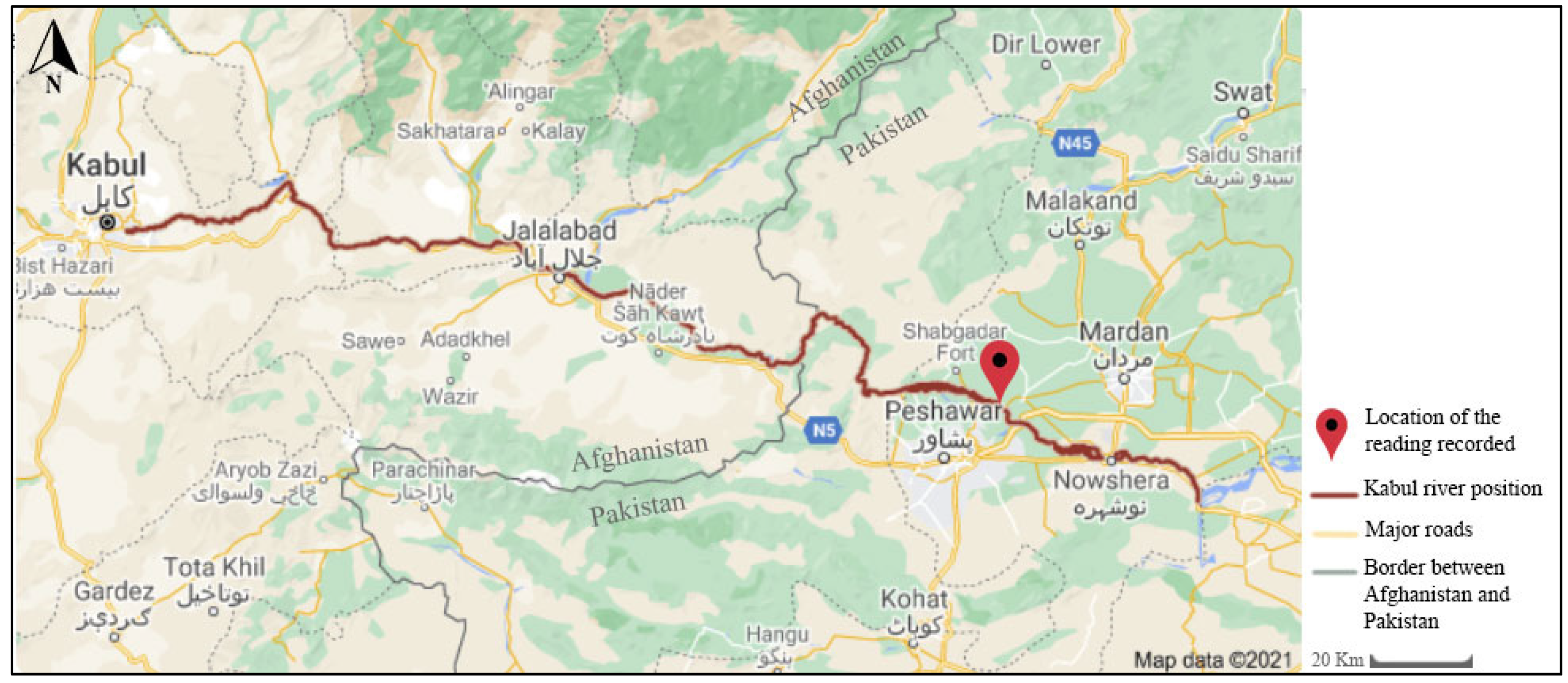
Figure 1. Kabul River position between Pakistan and Afghanistan (Google Maps).
Sustainability 13 10720 g001
Figure 2. Seasonal decomposition of the data set.
Sustainability 13 10720 g002
Figure 3. Methodology flowchart.
Sustainability 13 10720 g003
Figure 4. ARIMA forecasting summary.
Sustainability 13 10720 g004
Figure 5. Comparison of actual and forecasted value.
Sustainability 13 10720 g005
Figure 6. Comparison of overall ARMA models.
Sustainability 13 10720 g006
Figure 7. Residual analysis for the selected model.
Sustainability 13 10720 g007
Figure 8. Top 20 models based on AIC.
Sustainability 13 10720 g008
Figure 9. Water flow forecasting from 2011 to 2030.
Sustainability 13 10720 g009
Figure 10. Error comparison of actual and predicted error in the model.
Sustainability 13 10720 g010
Table 1. Error analysis using selected parameters.
ModelModel Fit Statistics
R-SquaredRMSEMAPEMAE
Water_level_10.92225.25320.11014.188
Publisher’s Note: MDPI stays neutral with regard to jurisdictional claims in published maps and institutional affiliations.