Observational Scale Matters for Ecosystem Services Interactions and Spatial Distributions: A Case Study of the Ussuri Watershed, China

Abstract

Understanding how observational scale affects the interactions and spatial distributions of ecosystem services is important for effective ecosystem assessment and management. We conducted a case study in the Ussuri watershed, Northeast China, to explore how observational scale (1 km to 15 km grid resolution) influences the correlations and spatial distributions of ecosystem services. Four ecosystem services of particular importance for the sustainable development of the study area were examined: carbon sequestration, habitat provision, soil retention, and water retention. Across the observational scales examined, trade-offs and synergies of extensively distributed ecosystem services were more likely to be robust compared with those of sparsely distributed ecosystem services, and hot/cold-spots of ecosystem services were more likely to persist when associated with large rather than small land-cover patches. Our analysis suggests that a dual-purpose strategy is the most appropriate for the management of carbon sequestration and habitat provision, and cross-scale management strategies are the most appropriate for the management of soil retention and water retention in the study area. Further studies to deepen our understanding of local landscape patterns will help determine the most appropriate observational scale for analyzing the spatial distributions of these ecosystem services.

1. Introduction

Understanding the impact of observational scale on the interactions and spatial distribution of ecosystem services is an integral part of mainstreaming the incorporation of ecosystem services knowledge into ecosystem management strategies at the science–policy interface [1,2,3]. In ecological studies, observational scale can be defined in several ways depending on the context. For example, in studies based on remote sensing and modeling, observational scale is usually described as having four components: (1) level of spatial detail, (2) numerical fraction, (3) spatial extent, and (4) process scale [4,5,6], which together indicate that ecological phenomena and objects each have their own distinct scale, or a range of scales, at which their characteristics and patterns are best observed [7,8]. An example to clarify the importance of observational scale selection is the competition between individual plants, which can be observed and discussed at the habitat scale but not at the regional or global scale [9,10]. At these larger scales, the break-out of pests or diseases (regional scale) and climate change (global scale) are more suitable topics for observation [11].

Ecosystem services, which, broadly speaking, are the benefits humans receive from the natural environment, are examples of ecological phenomena that have distinct observational scales at which their dynamics can be most efficiently observed and understood. In the context of ecosystem service assessment, observational scale is usually defined as the scale at which samples are collected from the ecosystem service [8]. However, if observational scale is assumed to comprise several hierarchical levels, with each level associated with a scale break [9,10], it can be expected that an ecosystem service could have different characteristics at different observational scales. Recently, there has been increased interest in the issue of appropriate observational scale selection, which has resulted in the terms “scale effect” and “scale dependence” being used to describe the differences in ecological patterns and processes when observed at different scales [12,13]. However, despite ecosystem services currently being observed at many different observational scales [2], the effects of observational scale on ecosystem service assessment remain under-explored [8].

Identifying strategies that favor the management of multiple ecosystem services is an issue that is impacted by observational scale selection because ecosystem service management practices are developed based on feedback obtained from direct observation of ecosystem services [14,15,16]. Some scholars have recommended that ecosystem service assessments be made at the spatial scale where decision making occurs (e.g., at the local, subnational, national, regional, continental, or global scale) to provide assessments that are relevant to pre-defined social concerns [17]. However, such social concerns often span multiple spatial scales, and addressing those concerns requires an in-depth understanding of the complexities associated with multi-scale assessments [18]. Thus, elucidating how to identify the most appropriate observational scales at which to conduct ecosystem service assessments remains an important concern in the area of ecosystem services management.

Recently, a study in northeast China has suggested the need to reduce the ecosystem and service losses resulting from inappropriate policymaking and to improve the effectiveness of ecosystem management in the area [19]. However, a simple tally of ecosystem services would not reveal which factors are most important in this regard. Sometimes, factors that hamper the effectiveness of ecosystem management could be the intrinsic trade-offs among ecosystem services that were not anticipated during the management design phase [1]. Typical trade-offs among ecosystem services could occur across observational scales [20]. For example, strengthened food production observed at the site scale could impact habitat quality at a broader observational scale and potentially threaten water quality when observing at the watershed scale [21]. Thus, comprehending the impact of observational scale on ecosystem services’ interactions is crucial for promoting the efficiency of ecosystem management.

In previous ecological studies, the concept of hot/cold-spots has been used to delineate areas of ecological importance [22]. In the context of ecosystem service assessment, hot-spots indicate areas with a high concentration of ecosystem service value, whereas cold-spots indicate the contrary. Greater understanding of the hot/cold-spots of ecosystem services has led to the spatial distributions of ecosystem services becoming essential topics of research [8,21]. However, most previous studies have used administrative divisions or the original resolution at which the data were collected as the observational scale rather than taking a multi-scale approach, which may have distorted the study outcomes [8]. Therefore, improving our understanding of how observational scale affects the spatial distributions of ecosystem services is expected to contribute to the development of improved ecosystem service management strategies.

One approach to better understand observational scales’ impact on ecosystem services is to examine the robustness of ecosystem service assessments across various observational scales and determine how the characteristics of each ecosystem service are influenced by observational scale. Here, taking the Ussuri watershed in Northeast China as the study area, we examined how observational scale affects four ecosystem services in the area. For our observations, instead of using a conventional administrative scale (e.g., county, township), we used grids with resolutions ranging from 1 to 15 km. We then used our data to examine the changes in correlations between pairs of ecosystem services at increasing observational scales and how ecosystem service distributions react to different observational scales. Based on our findings, we discuss policy-relevant implications of choosing a specific scale for ecosystem service observation and assessment.

2. Data and Methods

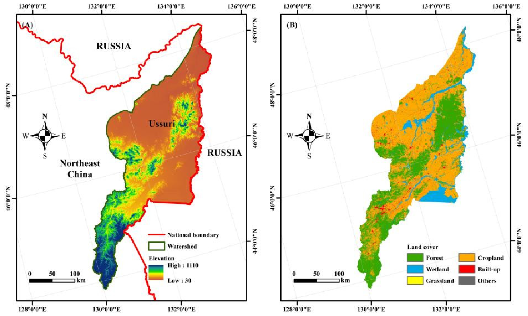
2.1. Study Site and Ecosystem Services

The Ussuri watershed in the Northern China Plain covers an area of approximately 61,460 km² and comprises a range of land covers and natural habitats, although it is predominantly plain in character (Figure 1A). The region is dominated by cropland (approx. 55% of the watershed in 2015) followed by green spaces (grassland, forest, and wetland; approx. 40% in 2015), but it also contains sparsely distributed rural and urban settlements (approx. 2.5% in 2015). The region is a typical peri-urban agricultural landscape that has been subjected to progressively industrialized farming, settlement development growth, and tourism exploitation (Figure 1B). A total of 15 cities/counties are entirely or partially located in the watershed, giving it a population of about 3,700,000. The Ussuri watershed is the largest component of the Sanjiang Plain (the largest marsh area in China and an important grain production base). However, the region has experienced tremendous wetland loss since the 1950s [23,24] and has been the recipient of strict management attention since 2000 [19,25,26].

Management for the rational and sustainable use of resources in the watershed is overseen by an assortment of government and public institutions. Alternative livelihood activities have been jointly implemented by the government of Heilongjiang, the Asian Development Bank, and the Global Environmental Facility to offer support and build consensus on common objectives for the management and use of forest/wetland resources, recognizing that the success of management strategies ultimately rests on the involvement of individuals [26]. The National Wetland Conservation Project of the National Forestry Administration is presently overseeing wetland resources management and is therefore responsible for the management framework [27].

Ecosystem services in the Ussuri watershed and adjacent regions are frequently mentioned in the literature, providing methodologies and data for diagnosing management problems [19,28,29]. In the present study, we examined four ecosystem services (i.e., carbon sequestration, habitat provision, water retention, and soil retention) that are related to the main concerns addressed by present ecosystem management strategies in the watershed (i.e., climate change mitigation, habitat rehabilitation, and headwater protection) [27].

Figure 1. Maps of the study site and elevation (m) (A) and land cover in 2015 (B). Forest: mixed forest, deciduous broadleaf forest, deciduous conifer, deciduous shrub, evergreen conifer, evergreen shrub, and tree garden; wetland: lake, reservoir, river, tree wetland, shrub wetland, herbaceous wetland, and canal; grassland: temperate steppe, tussock, and lawn; cropland: paddy field and dry farmland; built-up area: mine, transportation network, and settlements; other: barren land and desert [28].

Figure 1. Maps of the study site and elevation (m) (A) and land cover in 2015 (B). Forest: mixed forest, deciduous broadleaf forest, deciduous conifer, deciduous shrub, evergreen conifer, evergreen shrub, and tree garden; wetland: lake, reservoir, river, tree wetland, shrub wetland, herbaceous wetland, and canal; grassland: temperate steppe, tussock, and lawn; cropland: paddy field and dry farmland; built-up area: mine, transportation network, and settlements; other: barren land and desert [28].

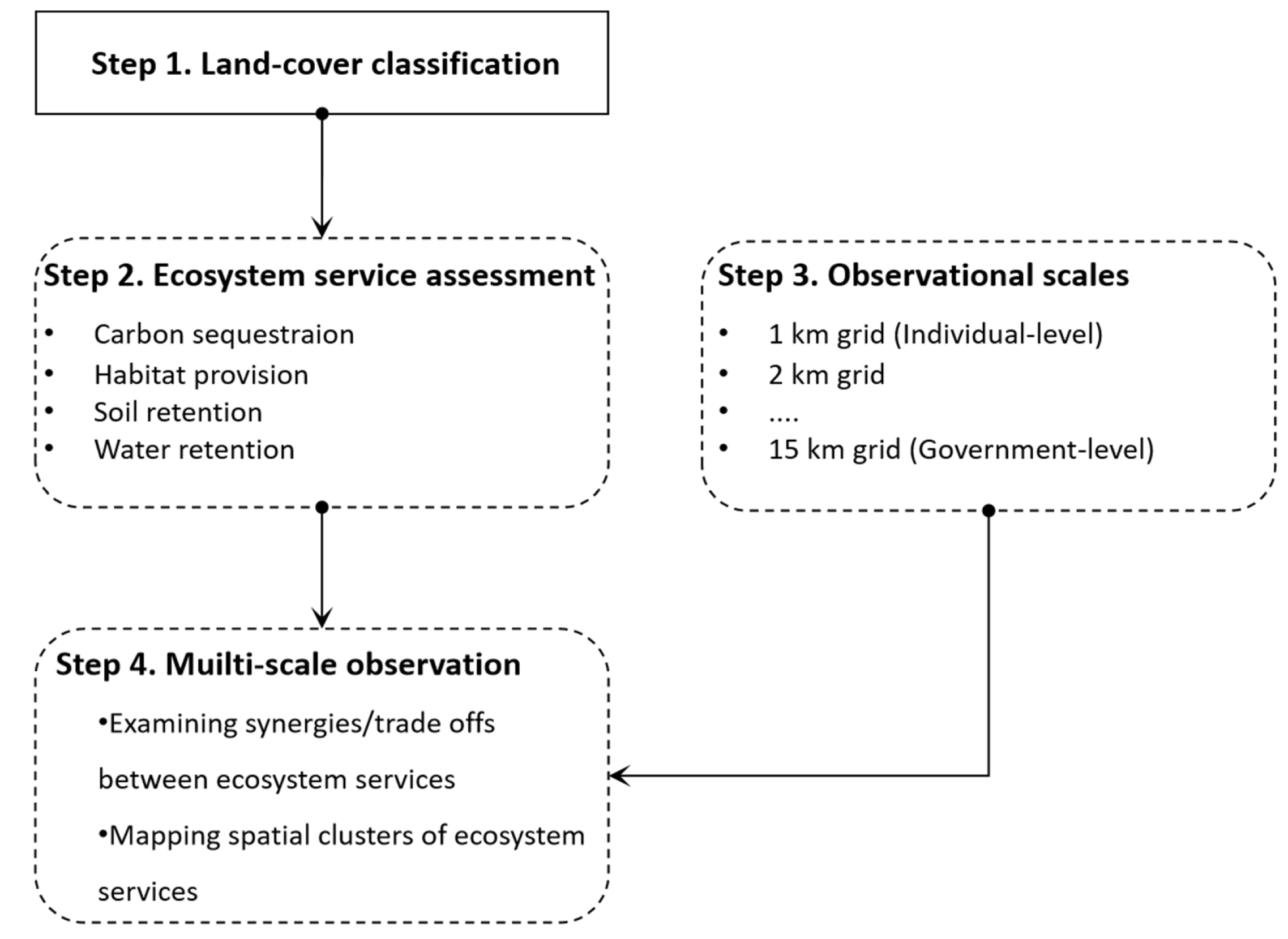
2.2. Methodological Steps

Figure 2 summarizes the methodological steps of estimating and analyzing ecosystem services across varied observational scales. The following sub-sections describe each step in detail.

2.3. Land-Cover Classification

Panchromatic images with 15/30 m spatial resolution collected in 2015 by the LANDSAT Enhanced Thematic Mapper Plus (NASA) and Operational Land Imager (NASA) were used as the source data for land-use classification (

Table 1. Descriptions of data used in land cover classification and ecosystem service assessment. All the websites were accessed on 16th April 2020).

Data	Resolution	Type	Data Sources
Satellite image	15/30 m	Raster	Geospatial Data Cloud (http://www.gscloud.cn).
Precipitation	1 km	Raster	National Meteorological Information Center (http://data.cma.cn/user/toLogin.html)
Daily minimum/ maximum temperature	1 km	Raster	National Meteorological Information Center (http://data.cma.cn/user/toLogin.html)
DEM	30 m	Raster	Geospatial Data Cloud (http://www.gscloud.cn).
Soil features	1 km	Raster	National Earth System Science Data Center
Carbon density	-	Text	Reference: Xiang et al., 2020.

). Cloudless satellite images (cloud coverage < 8%) collected in July, August, and early September were used for object-based classification. A total of 25 land-cover types were identified by using the multi-resolution segmentation and object-based classification approach of Mao et al. [19]. The accuracy of classification was assessed based on a total of 2388 historical ground-truth samples, affording an overall accuracy of 94%. Classification results were further compared with the land-use maps presented in recent studies to guarantee the applicability of the results for ecosystem service calculation [28,29,30]. For the quantification of ecosystem services, we used the original land-cover map with 25 land-cover types; for clearer display, the land-cover map for 2015 was further re-classified into six major land-cover types (forest, wetland, grassland, cropland, built-up area, and other) using the classification system of Wang et al. [28] (Figure 1B).

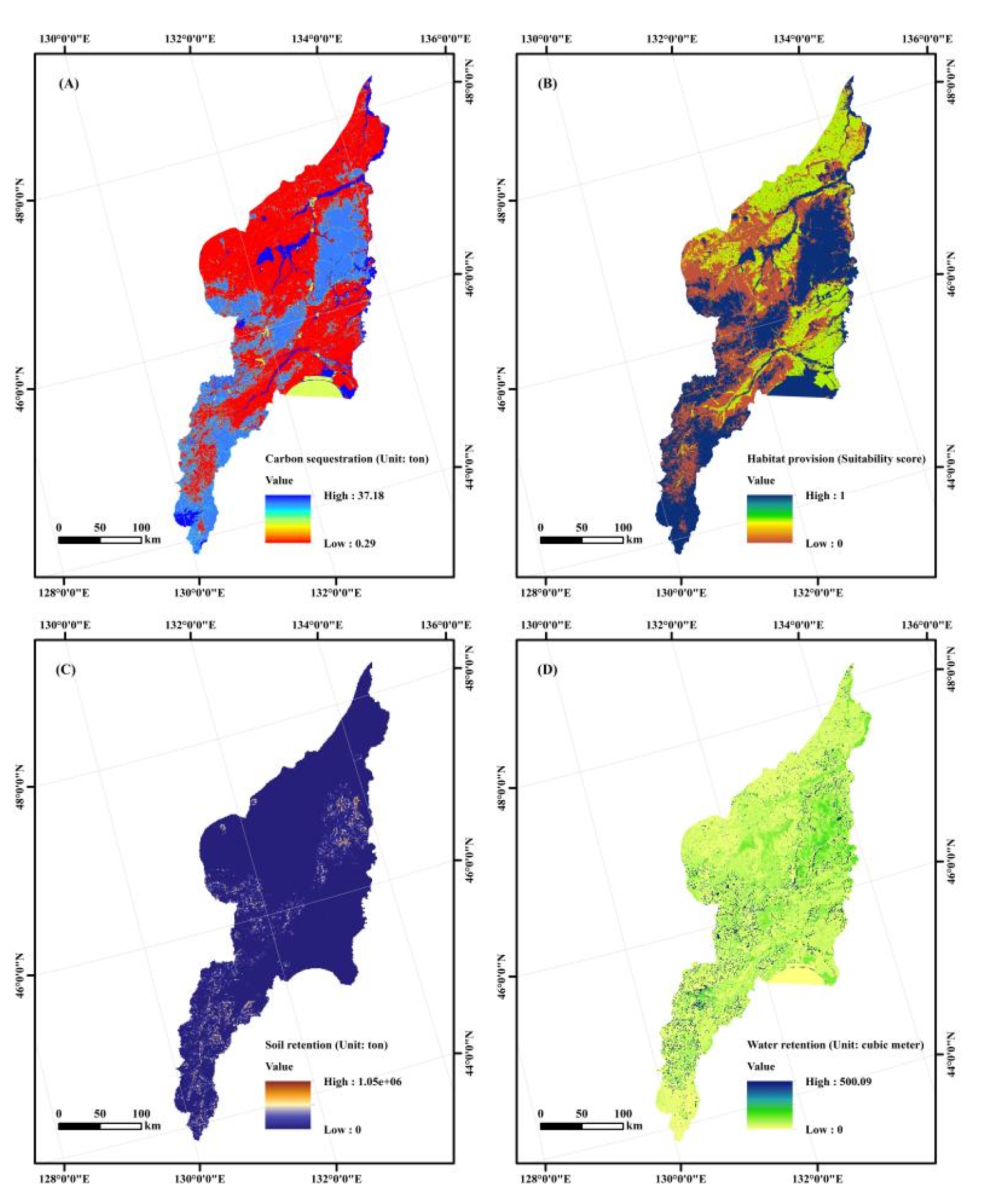
2.4. Quantification of Ecosystem Services

2.4.1. Carbon Sequestration

Carbon sequestration service (CS) measures the capture and secure storage of carbon dioxide that would otherwise be emitted to, or remain, in the atmosphere and is of great importance to tackling global warming. We used the Carbon module of InVEST 3.2.0 to generate a distribution map of carbon sequestration in the study area [31] (Figure 3A). The amounts of carbon stored in four carbon pools (above-ground biomass, below-ground biomass, soil, and litter layer organic matter) for all land cover types was determined by using the formula:

$$C_{total}={\displaystyle \sum }_i^n{C}_i\times S_i$$

(1)

where $C_{total}$ is the total amount of carbon sequestration in the Ussuri watershed, $C_i$ is the summed carbon density in the four carbon pools for land cover i, $S_i$ is the area of land cover i, and n is the number of land cover types we detected in the land-cover classification phase (n = 25). Carbon density data were obtained from Xiang et al. (Table 1) [32].

2.4.2. Habitat Provision

Habitat provision services (HP) are relevant to both permanent and transient populations of wildlife [33] and are extremely important for maintaining biodiversity [34]. We used the Habitat Quality module of InVEST to rate habitat quality on a scale of 0 to 1 (higher value indicates higher habitat quality) (Figure 3B). This module uses the following formula to estimate the spatial extent, vegetation type across a landscape, and state of degradation by combining information on land cover and threats to biodiversity:

$$Q_{xj}=H_j\left(1-\left(\frac{D_{xj}^z}{D_{xj}^z+k^z}\right)\right)$$

(2)

where $Q_{xj}$ is the habitat quality of pixel $x$ in land-cover type $j$, $H_j$ is the expert knowledge-based habitat quality score obtained from the InVEST 3.2.0 User’s Guide, ${\mathrm{D}}_{xj}$ is the state of degradation of pixel $x$ in land-cover type $j$ [31], and K is the half-saturation constant taken as 0.3 [29]. Note that the exponent Z assigned to ${\mathrm{D}}_{xj}$ and K refers to the scaling parameter, which was taken as 2.5 [29]. The data prepared for the estimation of $Q_{xj}$ comprise a land-cover map, the sensitivity of each land cover to each threat, and a list of threats and their features. The sensitivity of each land-cover type to each threat and the weight of their impact were obtained from Xiang et al. [29].

2.4.3. Soil Retention

Soil retention (SR) (Figure 3C), here defined as the difference between the potential worst case soil erosion under bare soil conditions and the actual soil erosion calculated by using the Universal Soil Loss equation [35], was calculated as follows:

$$SR=R\times K\times LS\times \left(1-C\right)$$

(3)

where $R$ is rainfall erosivity (MJ mm, ha⁻² ha⁻¹ yr⁻¹) (calculated based on daily precipitation), $K$ is soil erodibility (t h MJ⁻¹ mm⁻¹), $LS$ is slope length gradient factor (calculated based on DEM), and $C$ is the percentage of vegetation coverage. Data sources of daily precipitation, soil erodibility, and DEM are from the National Earth System Science Data Center (http://www.geodata.c, accessed 16 April 2020.) (Table 1).

2.4.4. Water Retention

Water retention service (WR) measures soil’s ability to retain water. A two-step process was used to estimate water retention (Figure 3D). First, water yield was calculated using the Annual Water Yield module of InVEST and the following formula [31]:

$$W{Y}_{total}={\displaystyle \sum }_n^i\left(P_{i }-AE{T}_i\right)\times A_i$$

(4)

where $W{Y}_{total}$ is annual total water yield (t yr⁻¹), $P_i$ is annual precipitation (mm), $AE{T}_i$ is evapotranspiration (mm), $A_i$ is area (km²), and i is the pixel of interest. The calculation of $W{Y}_{total}$ followed the detailed methods presented in InVEST 3.2.0 User’s Guide. We then used the value of $W{Y}_{total}$ to calculate the water retention capacity using the method of Wang et al. [36] as follows:

$$W{R}_{capacity}=\mathrm{MIN}\left(1, \frac{249}{V}\right)\times \mathrm{MIN}\left(1,\frac{0.9\times TI}{3}\right)\times \mathrm{MIN}\left(1,\frac{K_{sat}}{300}\right)\times W{Y}_{total}$$

(5)

$$\mathrm{TI}=\mathrm{Log}\left(\frac{Surface}{SoilDepth\times PercentSlope}\right)$$

(6)

where $W{R}_{capacity}$ is the annual average water retention capacity (mm); $V$ is the velocity coefficient, which is a constant value (dimensionless); $TI$ is the topographic index (dimensionless); and $K_{sat}$ is the saturated hydraulic conductivity (mm/d). “$Surface$” in Formula (6) is the number of grids in the watershed, “$SoilDepth$” is the soil thickness (mm), and “$PercentSlope$” is the slope percentage (Table 1). The calculation methods of $TI$ and $K_{sat}$ were referenced from Li et al. [37], and the data sources and biophysical parameters used in Formulas (4)–(6) were obtained from Xiang et al. [29].

2.5. Method of Analysis

2.5.1. Observational Scales

The observational scales employed in this study were developed on the basis of management scales (scales at which ecosystem management is formally implemented in the Ussuri watershed) and scale hierarchies [10]. The management scales were determined by identifying the principal managers of ecosystem services. Usually, principal managers of ecosystem services refer to individuals who are formally incentivized to engineer the landscape to manage the ecosystem, and the institutions that develop rules to regulate access to ecosystem services [8]. In the Ussuri watershed, the principal managers of ecosystem services were (1) farmers who grant part of their croplands for wetland and forest restoration or manage their farmland for soil condition and grain yield, and (2) the government bureau that supervises national nature reserves therein [19,26,29]. The management decisions and implementations often occur at the individual level, government level, or some compromised level between them. Therefore, the 1 km grid, which was considered to approximate the spatial scale at which individual land-use management occurs, was designated as the finest observational scale. Meanwhile, the 15 km grid, which was considered to approximate areas of land similar in size to the smallest nature reserve (the Qixinghe wetland reserves that covers an area of 208 km²) and the spatial scale at which national directives and local interventions are applied, was designated as the coarsest observational scale. In addition, 13 intermediate observation scales (scales between the 1 km and 15 km grids where sampling is conducted and measurements are taken) were added to clarify how features of ecosystem services react to changes in observational scale [8,38]. These intermediate observational scales were simulated with a 1 km grid interval (i.e., from 2 to 14 km grid resolution). All 15 grids were generated in ArcGIS 10.7 using the Fishnet tool.

2.5.2. Correlations between Ecosystem Service Pairs

A correlation analysis was conducted to examine the suitability of using a dual-purpose management strategy (a management strategy that regulates two ecosystem services at the same time) for each pair of ecosystem services. We hypothesized that (1) a dual-purpose management alignment will occur at an observational scale when there is synergy between a pair of ecosystem services, indicating that the two ecosystem services can be managed simultaneously, and (2) a dual-purpose management mismatch will occur at an observational scale when there is a trade-off or no correlation between a pair of ecosystem services, indicating that the two ecosystem services cannot be managed simultaneously.

Pearson’s parametric correlation test was performed in IBM SPSS 22 to identify potential synergies and trade-offs among pairs of ecosystem services. Min max normalization was applied to nondimensionalize the data before analysis. The Shapiro–Wilk test was used to verify the normality of the data before the correlation analysis. If the coefficient between pairwise ecosystem services was significant (p < 0.05), the correlation was considered valid. A significant negative coefficient was considered to indicate the existence of a trade-off (one ecosystem service increases while the other decreases), and a significant positive correlation was considered to indicate the existence of a synergy (both ecosystem services increase) [39]. The correlation analysis was performed at each of the predetermined observational scales to examine the changes in ecosystem service interactions across observational scales. When using the coarsest observational scale (15 km grid), the maximum sample size of ecosystem services was 229 in this study. Therefore, the ecosystem service samples at each observational scale were all set to 229 to avoid the impact of varied sample sizes on the significance test. The sampling points at all observational scales except for the coarsest observational scale were randomly selected using ArcGIS 10.7 and manually edited to avoid an over-concentrated distribution.

2.5.3. Spatial Patterns of Ecosystem Services

To quantify the spatial patterns of the ecosystem services, we used Anselin’s local Moran’s indicator [40]. This indicator is used to decompose a global statistic into its constituent parts [40], and then each part is classified as a hot-spot (high–high clusters), cold-spot (low–low clusters), outlier (high–low or low–high clusters), or non-significant spot. We used this approach to identify areas of the watershed where different management approaches could be successful [22]. The hot-spots indicated areas where high-value ecosystem services are highly aggregated, suggesting that a reactive management approach would be appropriate; the cold-spots indicated areas where low-value ecosystem services are highly aggregated, suggesting that a proactive management approach would be appropriate.

A step-wise process was used to analyze the spatial clusters of the ecosystem services. First, the spatially explicit evaluation of the ecosystem services derived by InVEST simulation was re-calculated in ArcGIS for all observational scales. Then, Anselin’s local Moran’s indicator [40] with queen contiguity was calculated in ArcGIS and compared at all observational scales. Finally, the hot/cold-spots were screened out and counted. A local regression (LOESS) curve fitting was performed to visualize the general trends as the observational scale was changed.

3. Results

3.1. Correlations between Ecosystem Service Pairs at Different Observational Scales

Correlation analysis revealed only one ecosystem service pair, CS–HP, with significant, high synergy at all observational scales (r = 0.860–0.923;

Table 2. Pearson correlation coefficients for pairs of ecosystem services at different observational scales. Synergies are shown in green, trade-offs are shown in red, and no correlations are shown in yellow. ** p < 0.01; * p < 0.05. CS, carbon sequestration; HP, habitat provision; SR, soil retention; WR, water retention.

	CS-HP	CS-SR	CS-WR	HP-SR	HP-WR	SR-WR
1 km grid	0.893 **	0.423 **	−0.127	0.373 **	−0.198	−0.191
2 km grid	0.894 **	0.386 **	−0.136	0.351 *	−0.211	0.026
3 km grid	0.891 **	0.331 *	−0.422 **	0.318 *	−0.555 **	−0.062
4 km grid	0.882 **	0.306 *	−0.398 **	0.296 *	−0.564 **	−0.031
5 km grid	0.877 **	0.253	−0.401 **	0.238	−0.580 **	0.004
6 km grid	0.875 **	0.244	−0.373 **	0.209	−0.551 **	0.120
7 km grid	0.874 **	0.253	−0.355 *	0.194	−0.540 **	0.173
8 km grid	0.873 **	0.254	−0.306 *	0.169	−0.499 **	0.187
9 km grid	0.869 **	0.291 *	−0.239	0.184	−0.459 **	0.253
10 km grid	0.868 **	0.302 *	−0.231	0.188	−0.448 **	0.304 *
11 km grid	0.867 **	0.322 *	−0.217	0.189	−0.442 **	0.335 *
12 km grid	0.860 **	0.301 *	−0.224	0.159	−0.471 **	0.380 **
13 km grid	0.862 **	0.309 *	−0.213	0.161	−0.452 **	0.375 **
14 km grid	0.864 **	0.323 *	−0.194	0.164	−0.440 **	0.427 **
15 km grid	0.923 **	0.674 **	0.288 *	0.630 **	0.181	0.613 **

). A mix of synergies and trade-offs were found for the other ecosystem service pairs depending on the observational scale.

Synergies were observed for CS–SR, HP–SR, and WR–SR. For CS–SR, low synergy was observed at 1–4 km grid resolution (r = 0.306–0.423) and 9–14 km grid resolution (r = 0.291–0.323), and high synergy was observed at 15 km grid resolution (r = 0.674). For HP–SR, low synergy was observed at 1–4 km grid resolution (r = 0.296–0.373) and high synergy was observed at 15 km grid resolution (r = 0.630). For WR–SR, low to high synergy was observed at 10–15 km grid resolution (r = 0.304–0.613).

Negative correlations, which indicate trade-offs between ecosystem services, were observed for CS–WR and HP–WR. For CS–WR, trade-offs were observed at 3–8 km grid resolution (r = −0.422 to −0.306) but synergy was observed at 15 km grid resolution (r = 0.288). For, HP–WR, trade-offs were observed at 3–14 km grid resolution (r = −0.580 to −0.440).

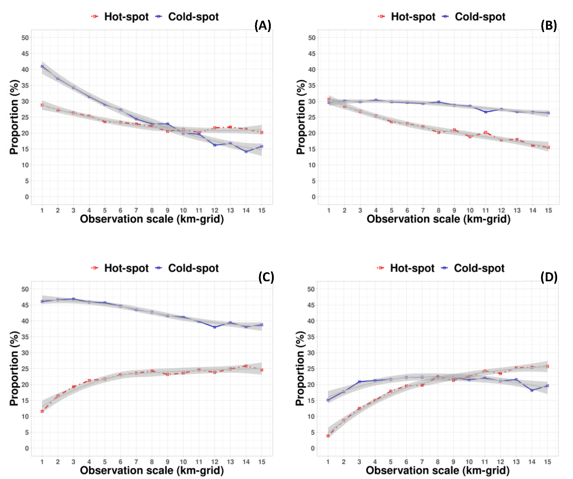
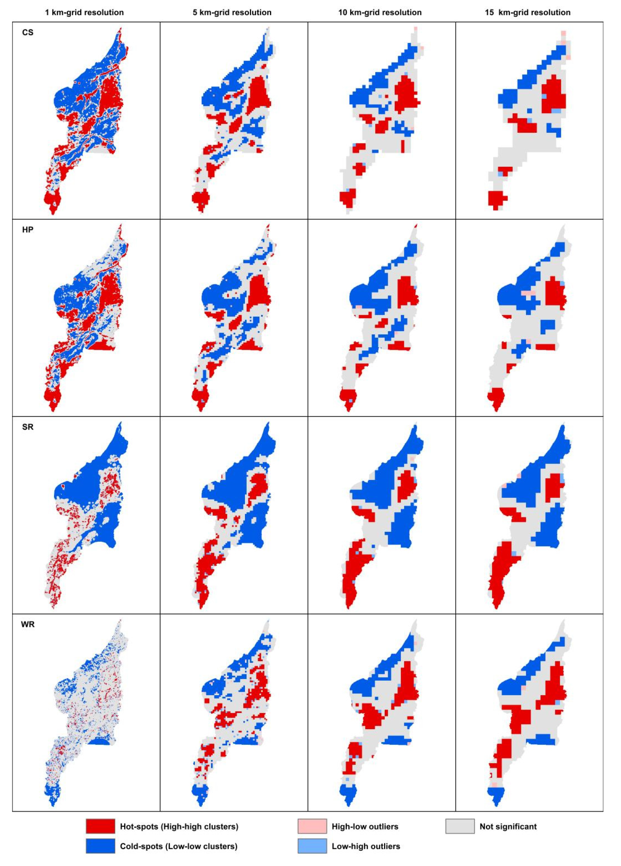
3.2. Spatial Distributions of the Ecosystem Services at Different Observational Scales

We used the local Moran’s indicator to examine the spatial distribution of each of the four ecosystem services across the 15 observational scales. Figure 4 shows the distributions of hot-spots (high–high clusters), cold-spots (low–low clusters), outliers (high–low or low–high clusters), and non-significant spots. When the observational scale was increased, adjacent grid areas of any cluster type were merged and then smoothed before the new grid area was assigned a new cluster type. This resulted in the scaling behavior of the different ecosystem service clusters across the observational scales being characterized as either merge–shrink or merge–expand. For example, for WR, small hot-spots were scattered across the study area at the finest observational scale (1 km grid resolution); however, as the observational scale was increased, these areas merged together and increased in size, resulting in a merge–expand behavior.

Figure 5 shows the changes in the proportion of land classified as hot/cold-spots for each ecosystem service with increasing observational scale; LOESS curves are shown to clarify the general trends. The proportion changes of 1 km vs. 15 km grid resolution observation were calculated. For CS, HP, and SR, the proportion of cold-spots decreased with increasing observational scale, with decreases of 25.2% for CS, 3.3% for HP, and 7.3% for SR (Figure 5A–C). In contrast, for WR, the proportion of cold-spots increased by 4.5% (Figure 5D). For CS and HP, the proportion of hot-spots decreased by 8.6% and 15.1%, respectively (Figure 5A,B), whereas for SR and WR, the proportion of hot-spots increased by 13.0% and 21.8%, respectively (Figure 5C,D).

Shifts in whether hot- or cold-spots were dominant were observed for CS, HP, and WR (Figure 5A,B,D). For CS and WR, there was a greater proportion of cold-spots compared with hot-spots at lower grid resolutions, but a greater proportion of hot-spots compared with cold-spots at higher resolutions; this reversal occurred at 10 km grid resolutions for CS and at 8 km grid resolution for WR. For HP, the proportion of hot-spots was greater than that of cold-spots at 1 km grid resolution, but this situation reversed from 2 km grid resolution.

4. Discussion

Understanding the spatial distributions and interactions of ecosystem services is crucial for the development of effective ecosystem service management strategies. The scales at which ecosystem services are observed or monitored fundamentally shape this understanding. Here, we conducted a case study of the area of the Ussuri watershed within the border of the People’s Republic of China to examine how observational scale affects the mapping of ecosystem services and their pairwise synergies and trade-offs. Based on our findings, we discuss how best to select the most appropriate observational scale for ecosystem service assessment and management.

4.1. Synergies and Trade-Offs across Observational Scales

First, we determined pairwise correlations among the four ecosystem services to examine how their correlations change with increasing observational scale (Table 2). The authors of previous case studies conducted for Quebec, Canada [8], and the Ningxia Hui Autonomous Region, China [12], concluded that most pairwise correlations are robust across different observational scales and that significant correlations are more often observed at finer than at coarser observational scales. However, based on our present data, we do not agree with these previous conclusions, although it must be noted that ecosystem service selection and the biophysical context of the study area must be taken into consideration when comparing the present and previous data.

In our analysis, we found that the correlation between CS and HP was robustly synergistic across all observational scales. Our distribution maps for CS and HP revealed that these ecosystem services are distributed extensively throughout the study area and are frequently coincided with certain types of land cover (Figure 3). For example, areas of high CS value and HP suitability score were found to be areas classified as forest and wetland, which is natural given that these two land-cover types are characterized by their large carbon pools and abundance of wildlife [19,41,42]. Turner et al. noted that land cover types with extensive distribution tend to change evenly across observational scales because the local configuration does not influence scaling [43]. We consider that Turner’s summing applies equally to correlations between ecosystem services that are extensively distributed.

In contrast to the distribution maps for CS and HP, those for SR and WR revealed that these ecosystem services were unevenly and sparsely distributed throughout the study area. Areas of high SR were primarily areas of forest at high elevation, and that of WR shared a similar distribution but appeared as more fragmented patches (Figure 3). In addition, we found that the correlations involving these ecosystem services were a mix of synergies, trade-offs, and no correlations (Table 2). For example, for CS–WR, trade-offs of various strengths were observed from 3 to 8 km grid resolution; no correlations were observed at 1, 2, and 9–14 km grid resolutions; and low synergy was observed at 15 km grid resolution.

Collectively, the results of our correlation analysis suggest that the distribution of an ecosystem service is an indicator of how robust its pairwise correlations are across observational scales; that is, correlations among extensively distributed ecosystem services are more likely to be robust, whereas those of ecosystem services with patchy distributions are more likely less robust, suggesting that more judicious selection of observational scale would be required when conducting assessments of these ecosystem services.

Assuming that observational scale equals the spatial scale at which future management occurs, our data suggest two implications with regard to the use of a dual-purpose ecosystem service management strategy. First, the robust synergy between CS–HP at all observational scales suggests that dual-purpose management of these two ecosystem services may be a cost-effective means of providing synergistic enhancements to both ecosystem services, and that such a management strategy could be applied at any scale. Evidence supporting our viewpoint could be found in several previous studies, where Zheng et al. [44] and Xiang et al. [29] have reported that widespread natural habitat restoration has increased biodiversity in the Sanjiang plain. The restoration of high-diversity ecosystems on degraded or abandoned land merits further implementation for its potential to provide increased CS [45].

Second, despite the present dual-purpose management of WR and SR in the Ussuri watershed by the Grain for Green Project [19], which is overseeing the reforestation of marginal cropland to reduce soil erosion and water loss, we only found synergies between these two ecosystem services at the coarser observational scales examined (10 to 15 km grid resolution; Table 2), suggesting that the current dual-purpose management approach is not suitable at all observational scales. Improving SR by improving erosion control in specific areas also improves WR [46,47]; however, WR often relies on large-scale landscape patterns and watershed dynamics [48,49,50]. These characteristics of the two ecosystem services are consistent with our findings of a dual-purpose management mismatch between WR–SR at the fine and intermediate scales. One means of resolving this mismatch could be to increase the number of soil erosion control sites in the Ussuri watershed to create a more extensive distribution pattern; however, soil erosion control is a costly investment when implemented over a sizeable spatial scale. Therefore, we suggest introducing a cross-scale strategy for the management of SR and WR [8]. That is, we suggest incentivizing the participation of individual managers or management institutions in improving WR via implementing erosion control, which will reduce the workload and financial burdens placed on government-level WR management. Meanwhile, the government-level managers need to carry out plans to specify the spatial extent in the Ussuri watershed to guide individual and institutional managers to put erosion control into effect. It is also noteworthy that the plans should be based on the in-depth knowledge of the local landscape and spatial pattern of ecosystem services.

Despite our observation of moderate synergies for CS–SR and HP–SR at the 15 km grid resolution, more low-level synergies and no-correlations occurred for them during the scaling-up of observation (Table 2). Further research is needed to explore the potential of dual-purpose management for such ecosystem service pairs in the Ussuri watershed.

4.2. Ecosystem Service Clusters at Different Observational Scales

Mapping hot/cold-spots provides straightforward information for determining where to implement different management options. Cold-spots are areas where there is a lower possibility of harvesting an ecosystem service, suggesting that the ecosystem service therein is better left undisturbed. In contrast, hot-spots are areas where there is a higher possibility of harvesting an ecosystem service, suggesting that the ecosystem service therein may potentially be harvested with high acceptance by management institutions and other stakeholders.

Here, we found that observational scale substantially influenced the spatial distributions of hot/cold-spots in two ways (Figure 4). First, increasing the observational scale altered the location and size of the hot/cold-spot clusters, such that the land-cover type associated with some of the clusters also changed. For example, whereas CS hot-spots associated with large patches of forest and cold-spots associated with continuous cropland were relatively preserved across the observational scales, those associated with wetland in the central part of the study area at fine observational scales (1–3 km grid resolution) had disappeared at the intermediate and coarse observational scales. Similar findings were also observed for HP, SR, and WR, although the clusters associated with continuous cropland, large patches of forest, and sizeable water bodies were relatively persistent across the observational scales.

Second, changing the observational scale altered the proportion of land covered by the cold/hot-spots, and for CS, HP, and WR, increasing the observational scale altered whether it was hot- or cold-spots that were the dominant cluster type (Figure 5). Both the trends and the spatial extent of the ecosystem service clusters varied at different observational scales. We speculate that regardless of whether or not an ecosystem service is extensively distributed throughout an area, observation at certain scales will fail to capture the real spatial pattern of hot/cold-spots because land-cover features shape the distribution of these clusters as well as how these clusters react at different observational scales. A widely used principle that emerged in the field of mapping ecosystem services is observing ecosystem services at the scale of administrative, policy, and management boundaries to facilitate the relevance between the assessment output and management decision making [8,19]. This principle implies that the mapping of ecosystem services should be based on the question being asked and the type of details required. We argue that, indeed, the assessment needs to match with the need of decision makers, but, more importantly, the assessment should capture the complexities of ecosystem services. Therefore, the selection of an appropriate observational scale for ecosystem service cold/hot-spots can only be interpreted by taking into consideration the social-ecological heterogeneity of the local landscape. The landscape pattern in the Ussuri watershed is a combined result of the gradual encroachment of cropland on wetland since the 1980s, the implementation of forest and wetland conservation measures around 2000 [19], and the watershed’s distance from the urban agglomeration of Harbin. Therefore, understanding the underlying mechanisms that shape local social-ecological conditions can help define the appropriate scales for observing the spatial patterns of ecosystem service hot/cold-spots.

We argue that, indeed, the assessment needs to match with the need of decision makers, but, more importantly, the assessment should capture the complexities of ecosystem services.

4.3. Methodological Limitations and Future Study

Many previous studies have elucidated the factors that affect the correlations and distributions of ecosystem services (e.g., the accuracy of input data and aggregation method used), but observational scale has not yet been examined [51,52,53]. We found here that the effects of changing observational scale are similar to those produced by smoothing to create an approximate function that captures important patterns in a data set while leaving out noise and outliers. That is, we found that when the observational scale was changed, data points of value were modified so that individual points higher in value than the adjacent points were reduced, and points that were lower in value than the adjacent points were increased, leading to compromised values. Therefore, observational scale should be considered a double-edged sword [47,54]. On the one hand, because it clearly determines the fitness and coarseness of the data and patterns that are obtained, it brings convenience to decision makers by letting the assessment results feed the management goal; on the other hand, it brings challenges with respect to accuracy because increasing the observational scale may introduce redundant or inaccurate data.

Other limitations of the present study are the simulation method and quality of input data used to measure the ecosystem services. The InVEST model provides a straightforward approach to map and monitor habitat quality that can be used as an estimate of biodiversity [55]. However, when there are multiple definitions of natural habitats and threats (i.e., habitat patches would be defined differently by large mobile wildlife compared to rare species of plants) [53], different spatial distributions or other land cover-based data may be obtained. Although we conducted our analysis using the best available data to provide qualified results, our use of average inventory values for carbon density associated with specific land covers and default model parameters in the WR and SR simulations may have failed to capture the effects of management types, climate factors, and geographic traits. In addition, validation is often absent in ecosystem service mapping and monitoring, so a better understanding of the uncertainties involved in the models used is needed [56].

Regarding future study, we suggest including more aspects of ecosystem services, such as the societal values and consumption of ecosystem services, in multi-observational scale analysis to select suitable observational scales [8,15]. The societal values of ecosystem services influence the rules and actions that alter the provision and access to ecosystem services [15], and the consumption of ecosystem services implies appropriate management incentives [8]. Comprehending how these aspects of ecosystem services vary across different observational scales allows identifying potential conflicts in ecological/environmental management, particularly among different stakeholders and managers, thereby building an effective, accountable, and inclusive framework to guarantee the sustainability of ecosystems in the Ussuri watershed.

5. Conclusions

Here, we present a case study conducted in the Ussuri watershed, Northeast China, in which we examined how observational scale affects ecosystem service assessment. We examined four ecosystem services (regulating and supporting services) at 15 observational scales (1 to 15 km grid resolution), which included two approximate scales at which ecosystem management is formally implemented. Correlation analysis revealed that ecosystem service distribution may be an indicator of the robustness of the correlation between pairs of ecosystem services across various observational scales. That is, a correlation is likely to be robust when an ecosystem service is extensively distributed across the study area (i.e., CS and HP in the present study), but not robust when an ecosystem service is sparsely distributed (i.e., SR and WR). Based on our findings, we suggest that a dual-purpose management strategy is most appropriate for the management of CS–HP in the Ussuri watershed, and that cross-scale management strategies are the most appropriate for the management of WR and SR.

The pattern of ecosystem service clusters (cold/hot-spots) across the various observational scales was associated with the size of land cover patches. Indeed, complex networks of ecosystem service clusters were observed in association with dispersed land covers at finer observational scales, but these networks became less complex, homogenous clusters at coarser scales. In contrast, the ecosystem service clusters associated with continuous land covers were persistent across the various observational scales. Thus, selecting an appropriate observational scale for delineating ecosystem service clusters should take into account the local landscape patterns and an understanding of local social-ecological complexity.

Though our results have the potential to improve the management decision making in ecosystem services, there are still several limitations that need to be addressed in future study. Technically, enhancing the sensitivity of the models used results in better accuracy of the input data, and the use of local parameters could help achieve a better estimation of ecosystem services. Moreover, including societal values and consumption of ecosystem services in the multi-observational scale analysis will bring better negotiation and coordination between stakeholders and managers at different scales, thereby ensuring the sustainable development of the Ussuri watershed.

References

1. Tallis, H.; Kareiva, P.; Marvier, M.; Chang, A. An ecosystem services framework to support both practical conservation and economic development. Proc. Natl. Acad. Sci. USA 2008, 105, 9457–9464. [Google Scholar] [CrossRef] [Green Version]
2. Malinga, R.; Gordon, L.J.; Jewitt, G.; Lindborg, R. Mapping ecosystem services across scales and continents–A review. Ecosyst. Serv. 2015, 13, 57–63. [Google Scholar] [CrossRef]
3. Costanza, R.; De Groot, R.; Braat, L.; Kubiszewski, I.; Fioramonti, L.; Sutton, P.; Farber, S.; Grasso, M. Twenty years of ecosystem services: How far have we come and how far do we still need to go? Ecosyst. Serv. 2017, 28, 1–16. [Google Scholar] [CrossRef]
4. Farina, A. Principles and Methods in Landscape Ecology, 1st ed.; Chapman & Hall: London, UK, 1998. [Google Scholar]
5. Goodchild, M.F. Models of scale and scales of modeling. In Modeling Scale in Geographical Information; Tate, N.J., Atkinson, P.M., Eds.; Willey & Sons: Chichester, UK, 2001; pp. 3–10. [Google Scholar]
6. Wu, H.; Li, Z.L. Scale issues in remote sensing: A review on analysis, processing and modeling. Sensors 2009, 9, 1768–1793. [Google Scholar] [CrossRef]
7. Emmett, B.A.; Cooper, D.; Smart, S.; Jackson, B.; Thomas, A.; Cosby, B.; Evans, C.; Glanville, H.; McDonald, J.E.; Malham, S.K.; et al. Spatial patterns and environmental constraints on ecosystem services at a catchment scale. Sci. Total Environ. 2016, 572, 1586–1600. [Google Scholar] [CrossRef]
8. Raudsepp-Hearne, C.; Peterson, G.D. Scale and ecosystem services: How do observation, management, and analysis shift with scale—Lessons from Québec. Ecol. Soc. 2016, 21, 16. [Google Scholar] [CrossRef] [Green Version]
9. O’Neill, R.V.; Gardner, R.H.; Milne, B.T.; Turner, M.G.; Jackson, B. Heterogeneity and Spatial Hierarchies; Kolasa, J., Pickett, S.T.A., Eds.; Ecological Heterogeneity; Springer: New York, NY, USA, 1991; pp. 85–96. [Google Scholar]
10. Wu, J. Hierarchy and scaling: Extrapolating information along a scaling ladder. Can. J. Remote Sens. 1999, 25, 367–380. [Google Scholar] [CrossRef] [Green Version]
11. Kremen, C. Managing ecosystem services: What do we need to know about their ecology? Ecol. Lett. 2005, 8, 468–479. [Google Scholar] [CrossRef]
12. Xu, S.N.; Liu, Y.F.; Wang, X.; Zhang, G.X. Scale effect on spatial patterns of ecosystem services and associations among them in semi-arid area: A case study in Ningxia Hui Autonomous Region, China. Sci. Total Environ. 2017, 598, 297–306. [Google Scholar] [CrossRef]
13. Zhang, Y.H.; He, N.P.; Loreau, M.; Pan, Q.M.; Han, X.G. Scale dependence of the diversity-stability relationship in a temperate grassland. J. Ecol. 2017, 106, 1227–1285. [Google Scholar] [CrossRef] [PubMed] [Green Version]
14. Fisher, B.; Turner, R.K.; Morling, P. Defining and classifying ecosystem services for decision making. Ecol. Econ. 2009, 68, 643–653. [Google Scholar] [CrossRef] [Green Version]
15. Reyers, B.; Biggs, R.; Cumming, G.S.; Elmqvist, T.; Hejnowicz, A.P.; Polasky, S. Getting the measure of ecosystem services: A social–ecological approach. Front. Ecol. Environ. 2013, 11, 268–273. [Google Scholar] [CrossRef] [Green Version]
16. Bennett, E.M.; Cramer, W.; Begossi, A.; Cundill, G.; Díaz, S.; Egoh, B.N.; Geijzendorffer, I.R.; Krug, C.B.; Lavorel, S.; Lazos, E.; et al. Linking biodiversity, ecosystem services, and human well–being: Three challenges for designing research for sustainability. Curr. Opin. Env. Sust. 2015, 14, 76–85. [Google Scholar] [CrossRef]
17. Gitay, H.; Raudsepp-Hearne, C.; Blanco, H.; Garcia, K.; Pereira, H. Assessment process. In Ecosystems and Human Well–Being. Volume 4, Multiscale Assessments; Capistrano, D., Samper, C., Lee, M.J., Raudsepp-Hearne, C., Eds.; Island: Washington, DC, USA, 2005; pp. 119–140. [Google Scholar]
18. Scholes, R.J.; Reyers, B.; Biggs, R.; Spierenburg, M.J.; Duriappah, A. Multi-scale and cross-scale assessments of social–ecological systems and their ecosystem services. Curr. Opin. Environ. Sust. 2013, 5, 6–25. [Google Scholar] [CrossRef]
19. Mao, D.H.; He, X.Y.; Wang, Z.M.; Tian, Y.L.; Xiang, H.X.; Yu, H.; Man, W.D.; Jia, M.M.; Ren, C.Y.; Zheng, H.F. Diverse policies leading to contrasting impacts on land cover and ecosystem services in Northeast China. J. Clean Prod. 2019, 240, 117961. [Google Scholar] [CrossRef]
20. Rodríguez, J.P.; Beard, T.D.; Bennett, E.M.; Cumming, G.S.; Cork, S.J.; Agard, J.; Dobson, A.P.; Peterson, G.D. Trade-offs across space, time, and ecosystem services. Ecol. Soc. 2006, 11, 28. [Google Scholar] [CrossRef] [Green Version]
21. Holland, R.A.; Eigenbrod, F.; Armsworth, P.R.; Anderson, B.J.; Thomas, C.D.; Heinemeyer, A.; Gillings, S.; Roy, D.B.; Gaston, K.J. Spatial covariation between freshwater and terrestrial ecosystem services. Ecol. Appl. 2011, 21, 2034–2048. [Google Scholar] [CrossRef] [PubMed] [Green Version]
22. Schröter, M.; Remme, R.P. Spatial prioritisation for conserving ecosystem services: Comparing hotspots with heuristic optimisation. Landsc. Ecol. 2016, 31, 431–450. [Google Scholar] [CrossRef] [PubMed] [Green Version]
23. Yan, F.; Zhang, S. Ecosystem service decline in response to wetland loss in the Sanjiang Plain, Northeast China. Ecol. Eng. 2019, 130, 117–121. [Google Scholar] [CrossRef]
24. Shi, S.X.; Chang, Y.; Wang, G.D.; Li, Z.; Hu, Y.M.; Liu, M.; Li, Y.H.; Li, B.L.; Zong, M.; Huang, W.T. Planning for the wetland restoration potential based on the viability of the seed bank and the land-use change trajectory in the Sanjiang Plain of China. Sci. Total Environ. 2020, 733, 139208. [Google Scholar] [CrossRef]
25. Day, K.A. China’s Environment and the Challenge of Sustainable Development, 1st ed.; Routledge: Armonk, NY, USA, 2005. [Google Scholar]
26. Asian Development Bank (ADB). Peoples’ Republic of China: Sanjiang Plain Wetland Protection Project; Asian Development Bank: Changchun, China, 2016. [Google Scholar]
27. Wang, Z.M.; Wu, J.G.; Madden, M.; Mao, D.H. China’s Wetlands: Conservation Plans and Policy Impacts. Ambio 2012, 41, 782–786. [Google Scholar] [CrossRef] [Green Version]
28. Wang, Z.M.; Mao, D.H.; Li, L.; Jia, M.M.; Dong, Z.Y.; Miao, Z.H.; Ren, C.Y.; Song, C.C. Quantifying changes in multiple ecosystem services during 1992–2012 in the Sanjiang Plain of China. Sci. Total Environ. 2015, 514, 119–130. [Google Scholar] [CrossRef] [PubMed]
29. Xiang, H.M.; Wang, Z.M.; Mao, D.H.; Zhang, J.; Xi, Y.B.; Du, B.J.; Zhang, B. What did China’s National Wetland Conservation Program Achieve? Observations of changes in land cover and ecosystem services in the Sanjiang Plain. J. Environ. Manag. 2020, 267, 110623. [Google Scholar] [CrossRef] [PubMed]
30. Song, K.S.; Wang, Z.M.; Du, J.; Liu, L.; Zeng, L.H.; Ren, C.Y. Wetland degradation: Its driving forces and environmental impacts in the Sanjiang Plain, China. Environ. Manag. 2014, 54, 255–271. [Google Scholar] [CrossRef]
31. Sharp, R.; Chaplin-Kramer, R.; Wood, S.; Guerry, A.; Tallis, H.; Ricketts, T. InVEST 3.2.0 User’s Guide. The Natural Capital Project. Stanford University, University of Minnesota; The Nature Conservancy; World Wildlife Fund: Stanford, CA, USA, 2015. [Google Scholar]
32. Xiang, H.X.; Jia, M.M.; Wang, Z.M.; Li, L.; Mao, D.H.; Zhang, D.; Cui, G.S.; Zhu, W.H. Impacts of land cover changes on ecosystem carbon stocks over the transboundary Tumen River Basin in Northeast Asia. Chin. Geogr. Sci. 2018, 28, 973–985. [Google Scholar] [CrossRef] [Green Version]
33. Groot, R.D.; Wilson, M.; Boumans, R. A Typology for the Classification Description and Valuation of Ecosystem Functions, Goods and Services. Ecol. Econ. 2002, 41, 393–408. [Google Scholar] [CrossRef] [Green Version]
34. Krauss, J.; Bommarco, R.; Guardiola, M.; Heikkinen, R.; Helm, A.; Kuussaari, M.; Lindborg, R.; Öckinger, E.; Pärtel, M.; Pino, J.; et al. Habitat fragmentation causes immediate and time-delayed biodiversity loss at different trophic levels. Ecol. Lett. 2010, 13, 597–605. [Google Scholar] [CrossRef] [Green Version]
35. Jiang, C.; Zhang, H.; Zhang, Z. Spatially explicit assessment of ecosystem services in China’s Loess Plateau: Patterns, interactions, drivers, and implications. Glob. Planet. Chang. 2018, 161, 41–52. [Google Scholar] [CrossRef]
36. Wang, Y.C.; Zhao, J.; Fu, J.W.; Wei, W. Effects of the grain for green program on the water ecosystem services in an arid area of China—Using the shiyang river basin as an example. Ecol. Indic. 2019, 104, 659–668. [Google Scholar] [CrossRef]
37. Li, M.Y.; Liu, T.X.; Luo, Y.Y.; Duan, L.M.; Zhang, J.Y.; Zhou, Y.J.; Scharaw, B. Pedo-transfer function and remote-sensing-based inversion saturated hydraulic conductivity of surface soil layer in Xilin river basin. Acta Pedol. Sin. 2019, 56, 90–100. [Google Scholar]
38. Wu, J.; Jones, K.B.; Li, H.; Loucks, O.L. Scaling and Uncertainty Analysis in Ecology: Methods and Applications; Springer: Berlin/Heidelberg, Germany, 2006. [Google Scholar]
39. Bennett, E.M.; Peterson, G.D.; Gordon, L.J. Understanding relationships among multiple ecosystem services. Ecol. Lett. 2009, 12, 1394–1404. [Google Scholar] [CrossRef]
40. Anselin, L. Local indicators of spatial association-LISA. Geogr. Anal. 1995, 27, 93–115. [Google Scholar] [CrossRef]
41. Chiang, L.C.; Lin, Y.P.; Huang, T.; Schmeller, D.S.; Verburg, P.H.; Liu, Y.L.; Ding, T.S. Simulation of ecosystem service responses to multiple disturbances from an earthquake and several typhoons. Landsc. Urban Plan. 2014, 122, 41–55. [Google Scholar] [CrossRef]
42. Liu, X.; Meng, M.; Wang, Q.; Zhou, X.H.; Zhao, Y.N. Economic mechanisms for oriental white stork conservation. Chin. J. Wild. life. 2019, 40, 240–246. [Google Scholar]
43. Turner, M.G. Disturbance and landscape dynamics in a changing world. Ecology 2010, 91, 2833–2849. [Google Scholar] [CrossRef] [PubMed] [Green Version]
44. Zheng, H.F.; Shen, G.Q.; Shang, L.Y.; Lv, X.G.; Wang, Q.; McLaughlin, N.; He, X.Y. Efficacy of conservation strategies for endangered oriental white storks (Ciconia boyciana) under climate change in Northeast China. Biol. Conserv. 2016, 204, 367–377. [Google Scholar] [CrossRef]
45. Yang, Y.; Tilman, D.; Furey, G.; Lehman, C. Soil carbon sequestration accelerated by restoration of grassland biodiversity. Nat. Commun. 2019, 10, 718. [Google Scholar] [CrossRef] [Green Version]
46. Conroy, M.; Allen, C.; Peterson, J.; Pritchard, L.; Moore, C. Landscape Change in the Southern Piedmont: Challenges, Solutions, and Uncertainty Across Scales. Conserv. Ecol. 2003, 8, 17. [Google Scholar] [CrossRef] [Green Version]
47. Lant, C.L.; Kraft, S.E.; Beaulieu, J.; Bennett, D.; Loftus, T.; Nicklow, J. Using GIS-based ecological–economic modeling to evaluate policies affecting agricultural watersheds. Ecol. Econ. 2005, 55, 467–484. [Google Scholar] [CrossRef]
48. Tscharntke, T.; Klein, A.M.; Kruess, A.; Steffan-Dewenter, I.; Thies, C. Landscape perspectives on agricultural intensification and biodiversity–ecosystem service management. Ecol. Lett. 2005, 8, 857–874. [Google Scholar] [CrossRef]
49. Jaarsveld, A.S.V.; Biggs, R.; Scholes, R.J.; Bohensky, E.; Reyers, B.; Lynam, T.; Musvoto, C.; Fabricius, C. Measuring conditions and trends in ecosystem services at multiple scales: The Southern African Millennium Ecosystem Assessment (SAfMA) experience. Philos. Trans. R. Soc. B 2005, 360, 425–441. [Google Scholar] [CrossRef] [PubMed] [Green Version]
50. Brauman, K.A.; Daily, G.C.; Duarte, T.K.; Mooney, H.A. The nature and value of ecosystem services: An overview highlighting hydrologic services. Annu. Rev. Env. Resour. 2007, 32, 67–98. [Google Scholar] [CrossRef]
51. Myers, N.; Mittermeier, R.A.; Mittermeier, C.G.; Fonseca, G.A.B.D.; Kent, J. Biodiversity hotspots for conservation priorities. Nature 2000, 403, 853–858. [Google Scholar] [CrossRef] [PubMed]
52. Schröter, M.; Rusch, G.M.; Barton, D.N.; Blumentrath, S.; Nordén, B. Ecosystem services and opportunity costs shift spatial priorities for conserving forest biodiversity. PLoS ONE 2014, 9, e112557. [Google Scholar]
53. Ceauşu, S.; Gomes, I.; Pereira, H.M. Conservation planning for biodiversity and wilderness: A real-world example. Environ. Manage. 2015, 55, 1168–1180. [Google Scholar] [CrossRef] [Green Version]
54. Martín-López, B.; Gómez-Baggethun, E.; Lomas, P.L.; Montes, C. Effects of spatial and temporal scales on cultural services valuation. J. Environ. Manag. 2009, 90, 1050–1059. [Google Scholar] [CrossRef]
55. Lindenmayer, D.B.; Barton, P.S.; Lane, P.W.; Westgate, M.J.; McBurney, L. An Empirical Assessment and Comparison of Species-Based and Habitat-Based Surrogates: A Case Study of Forest Vertebrates and Large Old Trees. PLoS ONE 2014, 9, e89807. [Google Scholar]
56. Schulp, C.J.E.; Burkhard, B.; Maes, J.; Vliet, J.V.; Verburg, P.H. Uncertainties in Ecosystem Service Maps: A Comparison on the European Scale. PLoS ONE 2014, 9, e109643. [Google Scholar] [CrossRef] [Green Version]
Figure 2. Diagram of methodologies used in this study.
Sustainability 13 10649 g002
Figure 3. Distribution maps for the four ecosystem services examined in the present study. (A) Carbon sequestration; (B) habitat provision; (C) soil retention; (D) water retention.
Sustainability 13 10649 g003
Figure 4. Spatial patterns of ecosystem service clusters (99% confidence interval) at four representative grid resolutions. CS, carbon sequestration; HP, habitat provision; SR, soil retention; WR, water retention.
Sustainability 13 10649 g004
Figure 5. Changes in the proportion of land classified as hot/cold-spots with increasing observational scale for the four ecosystem services. (A) Carbon sequestration. (B) Habitat provision. (C) Soil retention. (D) Water retention. Gray curves are fitted curves that indicate the general trend (95% confidence interval).
Sustainability 13 10649 g005