Article

Study on the Optical Properties of the Point-Focus Fresnel System

Department of Environmental Science and Engineering, University of Science and Technology of China, 96 Jinzhai Road, Hefei 230026, China
*
Author to whom correspondence should be addressed.
Sustainability 2021, 13(18), 10367; https://doi.org/10.3390/su131810367
Submission received: 22 July 2021 / Revised: 16 August 2021 / Accepted: 18 August 2021 / Published: 16 September 2021
(This article belongs to the Collection Sustainable Electric Power Systems Research)

Abstract

:
The characteristic analysis of the flux formed by the heliostat in the optical system is the basis in design and optimization of the whole system. In this paper, our research subject is a pilot installation of the point-focus Fresnel system, which is a new optical design between the tower system and the dish system. For the optical system, it is very important to accurately calculate the solar flux density distribution on the receiver plane. Aiming at the case that the focal length of the heliostat is not equal to the distance from the center of the heliostat to the center of the receiver plane, based on the projection, an approximate calculation method is proposed. Using the method to calculate the solar flux density distribution of the point-focus Fresnel system, and the results are compared with that calculated by SolTrace code, it is found that the solar flux density distribution of both is relatively consistent in shape and numerical value, which verifies the accuracy of the method and it can be used for design and optimization of the point-focus Fresnel system.

1. Introduction

With the environmental problems such as resource depletion and emission pollution caused by the extensive use of fossil fuels, the development of renewable energy has become a very urgent issue facing human society. Focused solar thermal power generation uses a low cost and high efficiency heat storage system, which can continuously generate electricity. It is the only continuous power generation technology that can be applied on a large scale at present [1].
Solar thermal power generation technologies work in a way that solar rays are focused and reflected to the specific receiver plane. Solar thermal power generation systems can be classified as linear Fresnel systems, dish systems, trough systems and tower systems depending on their different structures and focusing types. In this paper, a new design [2], named point-focus Fresnel system, also known as integrated azimuth tracking solar tower system, is studied. The optimized average efficiency is 20% higher than that of the traditional tower system, which is almost the same as that of the dish system.
For the optical system, it is very important to accurately calculate the solar flux density distribution on the receiver plane. The intercept factor can be obtained by calculating the flux density distribution [3], so as to optimize the design of the system. In addition, the solar flux at the receiver can be calculated to predict the temperature of the receiver and prevent damage caused by local overheating of the receiver [4,5]. The existing methods are mainly divided into two categories: the ray tracing method and the convolution integral method.
Based on the convolution integration method, Huang [6] developed a new flux density function for a focusing heliostat. The elliptical Gaussian model uses a Gaussian function to fit the heliostat image function and applies the elliptical Gaussian to describe optical error. The proposed function can directly calculate the flux density of various round or rectangular focusing heliostat on the image plane. In this paper, we use the Gaussian flux density function to calculate the flux density distribution of rectangular focusing heliostats on the image plane which is perpendicular to the central reflected ray, then the flux density distribution on the receiver plane is calculated through projection. We compare and validate the method with ray-tracing method.

2. Materials and Methods

2.1. The Point-Focus Fresnel System

Figure 1 shows the layout of the heliostats for the point-focus Fresnel system in which all of the heliostats and receiver are installed on an azimuth tracking device, multi heliostats are fixed to a horizontal shaft which rotate to track the solar elevation variance. It is an experimental system in building. The height of the tower is 2.5 m, the tilt angle of the receiver plane to the vertical line is 0°. The parameters for calculation of the heliostats are listed in Table 1.

2.2. Computational Methods

The image plane is perpendicular to the solar ray reflected by the center of the heliostat from the center of the sun. The Gaussian flux density function [6] is used to calculate the flux density on the image plane. The main computational steps are as follows:
(1)
The receiver plane is discretized into a grid of equidistant nodes;
(2)
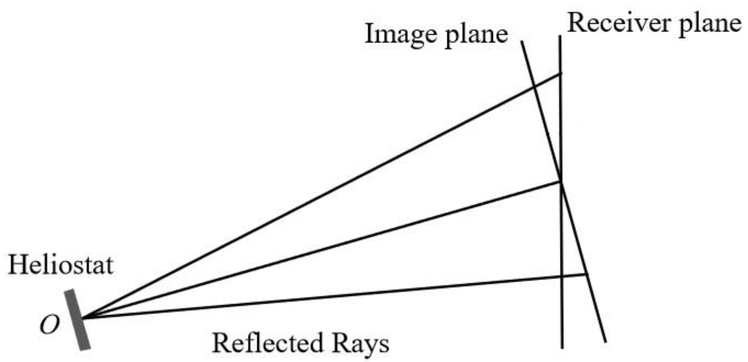
As shown in Figure 2, in order to calculate the flux density on the receiver plane, the grid nodes are projected onto the image plane in the direction to the center of the heliostat;
(3)
The flux density at projected point of the image plane is calculated by using the Gaussian flux density function which is shown in Table 2;
(4)
The flux density at a point of the receiver plane is proportional to that of its projected point of the image plane, although affected by the angel of incidence with the receiver plane, ω. The relationship between the flux density at a point of the receiver plane and the flux density at the projected point of the image plane satisfies:
F r e c e i v e r = F i m a g e × d i m a g e 2 d r e c e i v e r 2 × cos ω ,
where Freceiver is the solar flux density on the receiver plane, dreceiver is the distance from the grid nodes on the receiver plane to the center of the heliostat; Fimage is the solar flux density on the image plane, dimage is the distance from the grid nodes on the image plane to the center of the heliostat.
Where, H and W are the length and width of the actual rectangular heliostat, Am is the area of the heliostat, D is distance from a point at image plane to the reflection point, I0 is intensity of reflected light, f is the focus length of the heliostat, σslopexslopey respectively represent standard deviation of the slope errors at optical surface in transverse(x) and longitudinal(y) direction, σx,y, respectively represent standard deviation of the optical error distribution in x or y direction, σ ¯ s x , s y respectively represent the average standard deviations in the x or y direction, σi is the Gaussian function parameter of heliostat mirror image error, σsun represents the sunshape error, σtr is heliostat tracking error.
The Gaussian function parameters of a rectangular heliostat image are given as:
σ i x = W ( 1 cos λ ) 2 2 D           σ i y = H ( 1 cos λ ) 2 2 D ,
where, H and W are the length and width of the actual rectangular heliostat.
The average standard deviations in both directions are given as:
σ ¯ s y 2 = 4 σ s l o p e y 2 + ( 1 cos λ ) 2 8 c o s λ σ s l o p e x 2     σ ¯ s x 2 = 4 σ s l o p e x 2 + ( 1 cos λ ) 2 8 c o s λ σ s l o p e y 2
where λ is the incident angle of solar ray to the heliostat.

2.3. SolTrace Code

SolTrace [7] is a software package developed at the U.S. National Renewable Energy Laboratory to model solar power optical systems and analyze their performance. The code utilizes ray-tracing methodology. The user selects a given number of rays to be traced. Each ray is traced through the system while encountering various optical interactions. It replicates real photon interactions and therefore can provide accurate results for complex systems that cannot be modeled otherwise. The disadvantage is longer processing time. Accuracy increases with the number of rays traced and larger ray numbers means more processing time.

2.4. The Calculation Method of Average Absolute Difference for Flux Contours

In this paper, the flux density distribution of the point-focus Fresnel system is calculated by the elliptic Gaussian model and SolTrace code in several different situations. In order to analyze the reliability of the model, the average absolute difference between these two methods is calculated. The average absolute difference calculating formula of flux density distribution is as follows [6]:
R M S E = 1 u 1 v [ F s ( x u , y v ) F s   max F c ( x u , y v ) F c   max ] u v 1 ,
In the formula above, the receiver plane is discretized into a series of grids, in which u represents the number of discrete points in the X-axis direction, v represents the number of discrete points in the Y-axis direction, Fs and Fc represent the flux density calculated by SolTrace code and the proposed method, respectively.

2.5. Intercept Factor Calculation

We assume that there is a square receiver centered over the receiver plane [8], the intercept factor is the integration of the flux density over the receiver domains. As the side length of the square receiver changes, the value of the intercept factor is also different. The receiver plane is discretized into a certain number of cells, each cell has a length Δx and a width Δy. And the calculation formula of intercept factor is as follows:
f int = ( u , v ) F ( u , v ) × Δ x × Δ y E ,
where fint represents the intercept factor, F represents the solar flux density on the receiver plane, E represents the total energy reflected from the heliostat onto the receiver plane.

3. Results

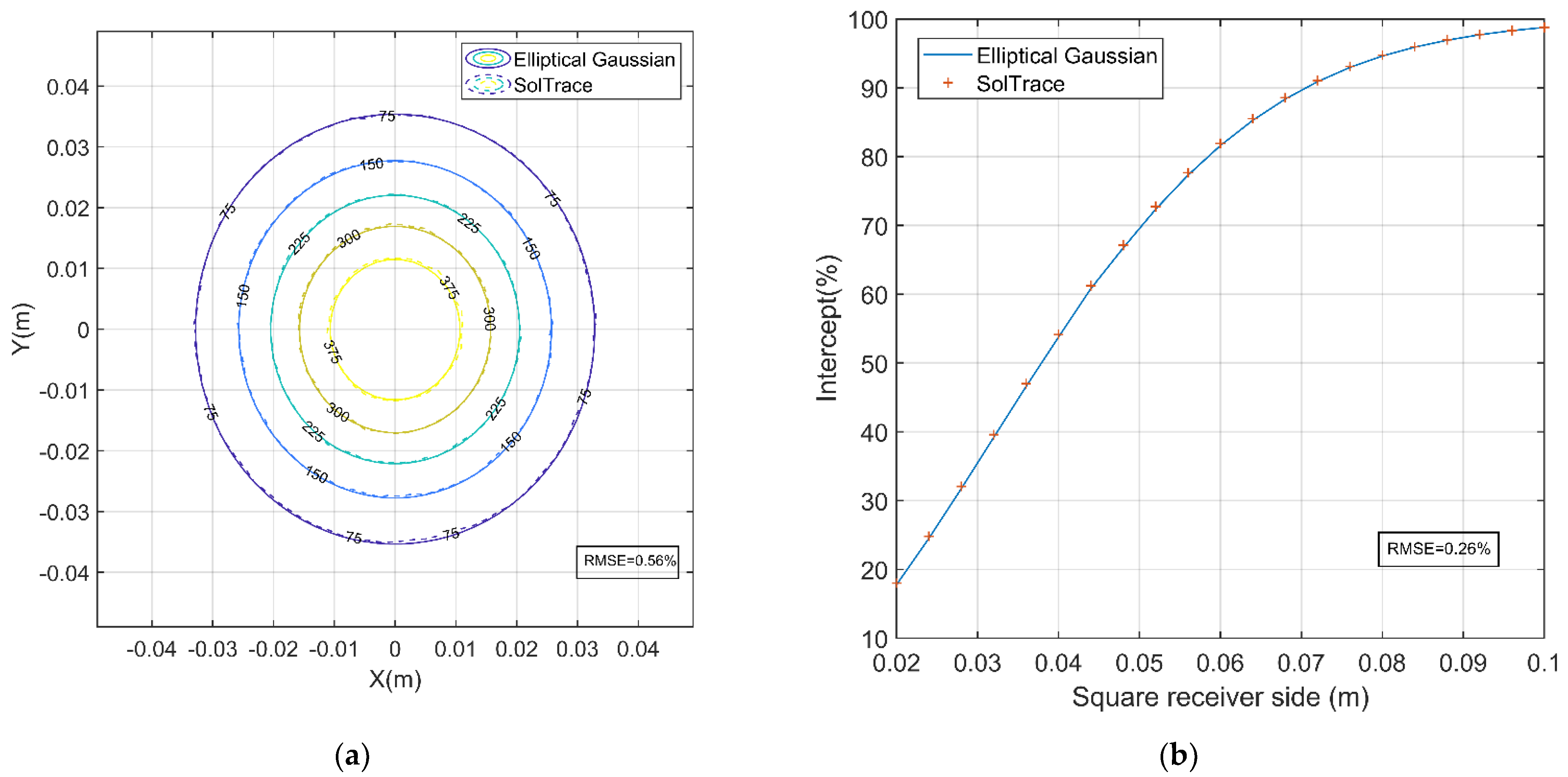
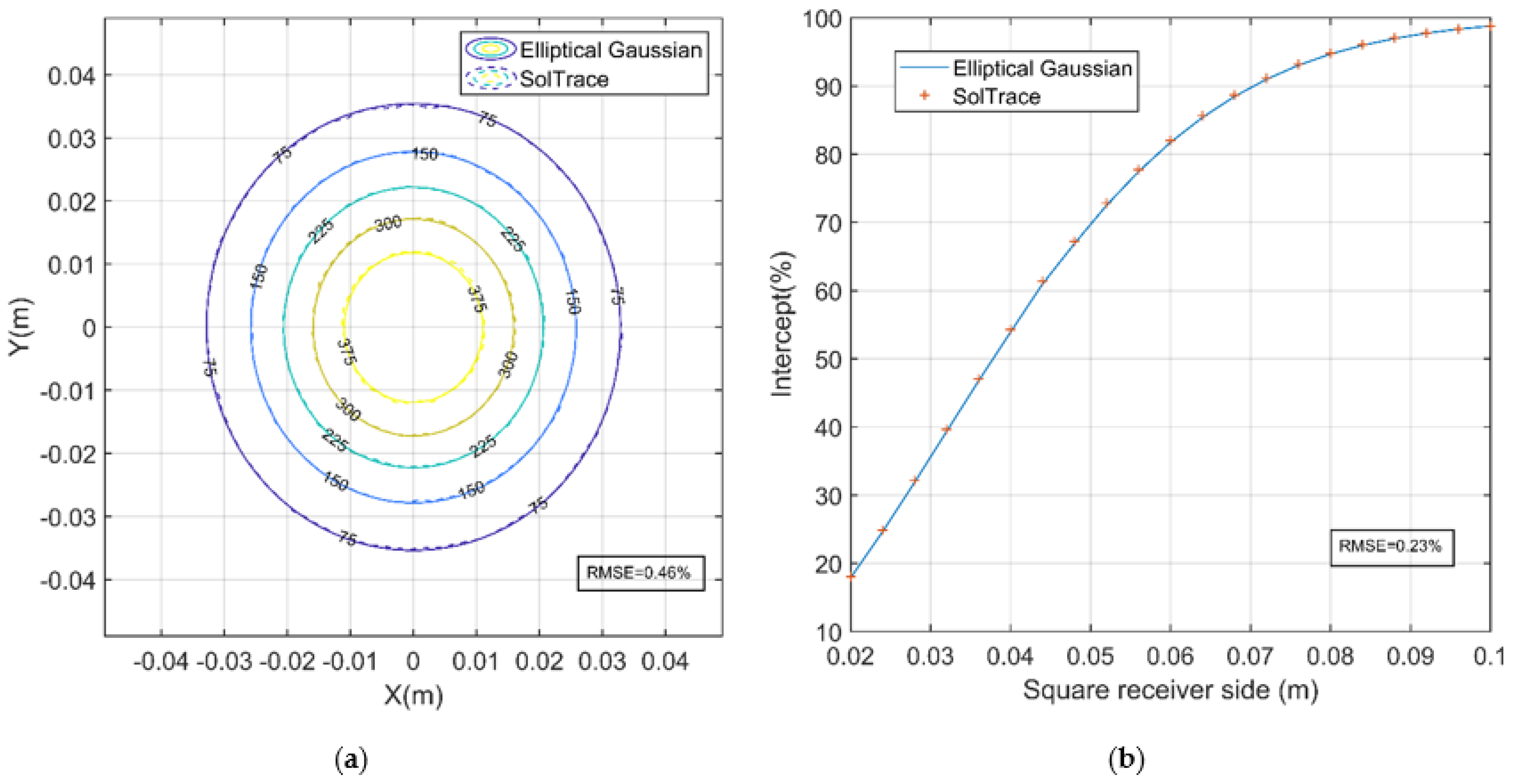
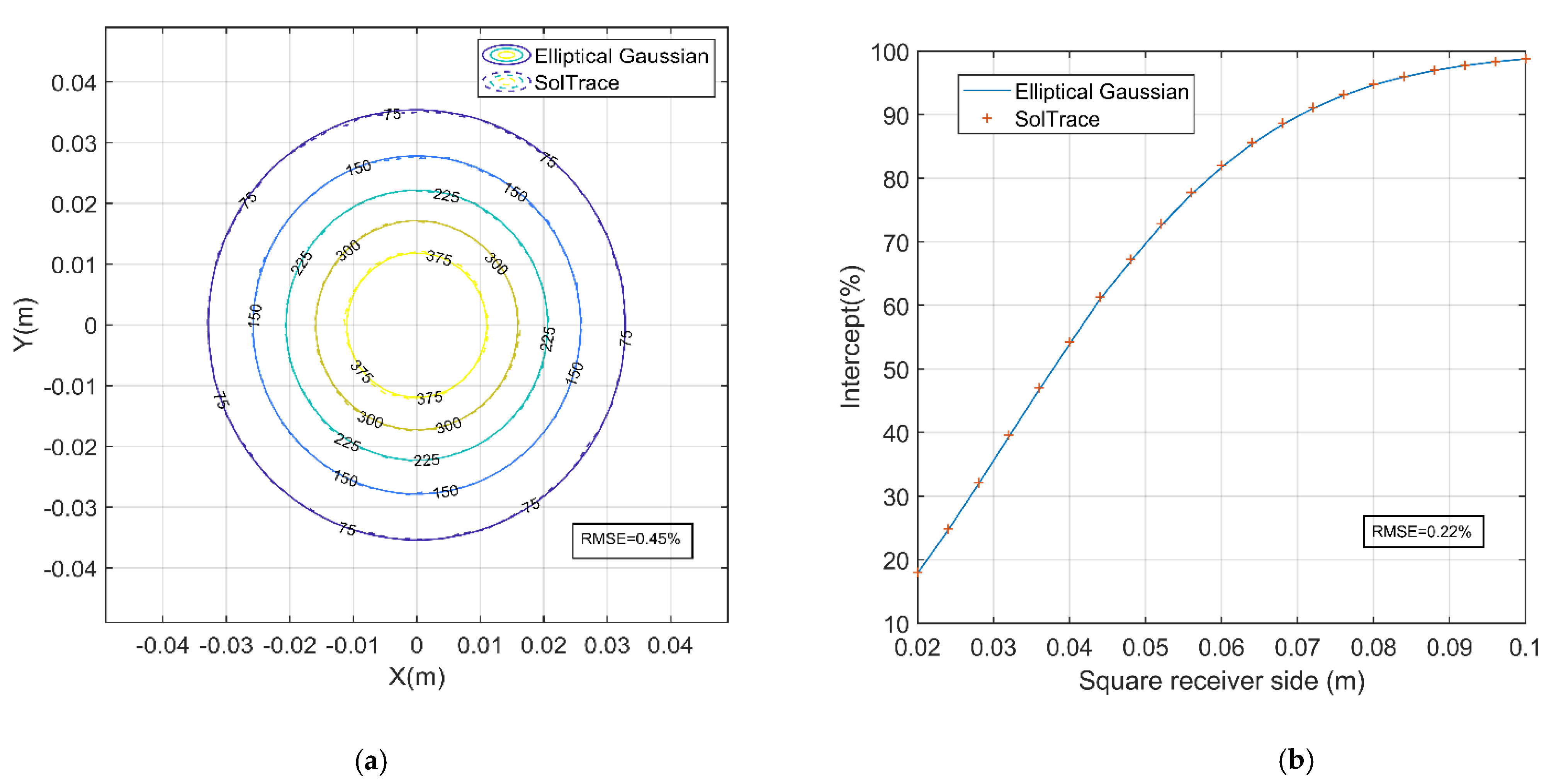
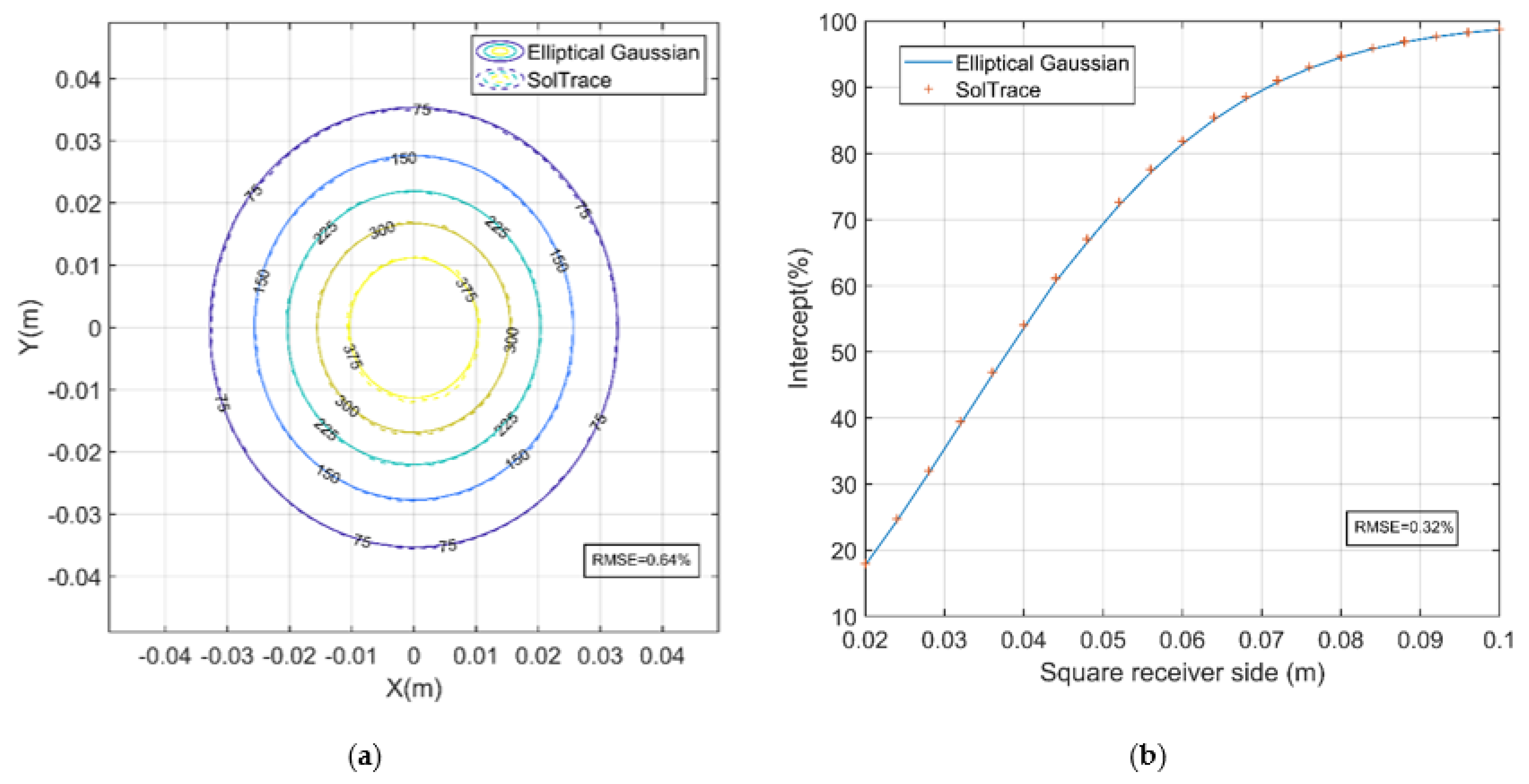
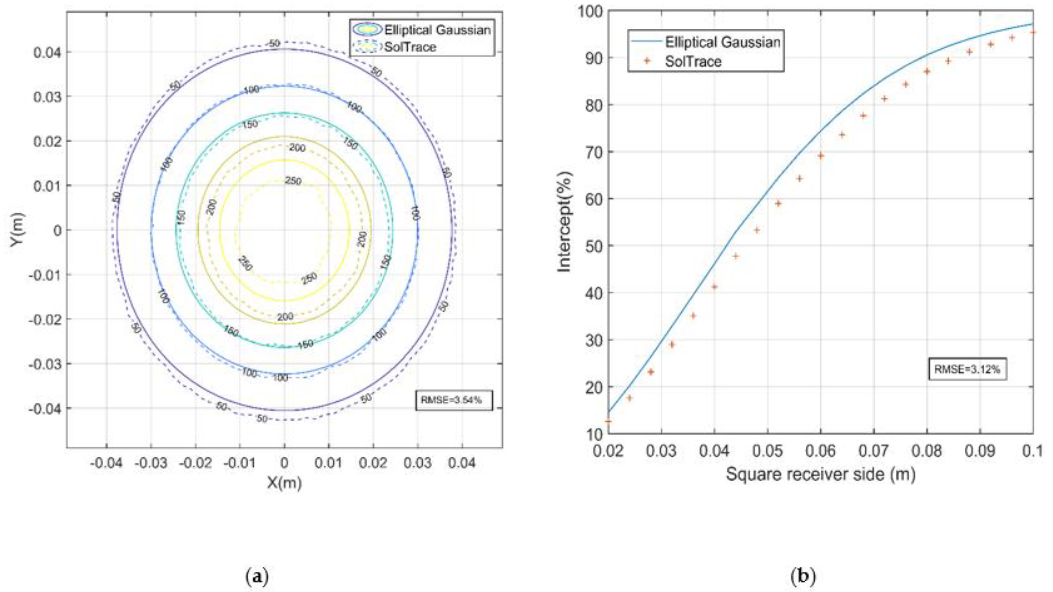
3.1. Model Validation: Compared to SolTrace

We use the Gaussian flux density function for a rectangular heliostat to calculate the solar flux density distribution formed by a single heliostat of the point-focus Fresnel system at different altitude angles of the Sun. The solar flux density distribution of the whole system is calculated by summation, and the results are compared with that calculated by SolTrace. In SolTrace code, the solar flux density calculated by 5 million random rays is accurate enough [9], so the desired number of ray intersections is set to 10 million. The origin of the global coordinate system is at the bottom of the receiver tower, with the positive X-axis pointing to the east, the positive Y-axis pointing to the north, and the positive Z-axis pointing to the zenith. The azimuth angle of the Sun is 0°, and other parameters are shown in Table 3.
Figure 3, Figure 4, Figure 5, Figure 6, Figure 7 and Figure 8 show the contours of solar flux density and intercepts which are calculated by SolTrace and the elliptical Gaussian model at the receiver plane, respectively.
The results, which show great consistency with that of SolTrace code, are listed in the Table 4.

3.2. The CPU Time of the SolTrace Code and Proposed Method

Simulations are carried out in an Intel(R) CoreTM i7-8700 microprocessor at 3.20 GHz equipped with 16 GB of RAM memory. Our code takes 0.22 s on average to execute, while SolTrace simulations with 10 million rays require an average time of 31.79 s. Figure 9 shows the CPU time for different numbers of rays, which indicates that the computational efficiency of the proposed method in this paper is higher than that of the SolTrace code.

4. Discussion

In summary, the results calculated by elliptical Gaussian model and SolTrace code are relatively consistent, the maximum error is 3.54%, and the minimum error is 0.45%. The largest differences correspond to the highest altitude angle of the Sun. The incidence angle of solar rays to the heliostat is about 25°, which is the largest in all cases. For the elliptical Gaussian model, according to the central limit theorem [10], when the parameters of the optical error distribution function is equivalent to or larger than that of Gaussian function parameters of heliostat image, the Gaussian distribution dominates the solar flux distribution function, and the error caused by the non-Gaussian part can be neglected. However, when the incident angle of solar ray to the heliostat is large, from the calculation equations of error parameters which is listed in Table 2, the Gaussian function parameters of rectangular heliostat image will also be large and it doesn’t satisfy the condition above, so the error would be larger.
Furthermore, the elliptical Gaussian model proposed by Huang is based on the convolution integration method, this method assumes that the length of the image formed by the heliostat on the image plane in the sagittal and tangential direction is proportional to the length of the heliostat with the same ratio ([11], p. 181). However, this hypothetical image of the heliostat is different from the actual one, therefore the convolution integration method itself has some errors. According to the geometrical optical knowledge [12], generally, the aberration is inversely proportional to the focal length and directly proportional to the size of the heliostat. Thus the larger the ratio of the focal length to the size of the heliostat, the less error between the present method and SolTrace code.
Besides, in the point-focus Fresnel system in this study, due to the fact the focal length of the heliostat is not equal to the distance from the heliostat to the receiver, the focal point is not on the receiver plane. The projection from the receiver plane to the image plane is different from the general case [9]. The method proposed in this paper assumes that all the rays are reflected from the center of the heliostat, the solar flux projection from the image plane to the receiver plane may increase prediction errors. In general, the closer the focal point is to the receiver, the less RMSE between these two methods.
The other minor error source of the proposed method are analyzed as follows:
  • The contribution to the reflected rays from the optical error of the heliostat is different in different positions of the heliostat [13]. However, proposed method in this paper assume that it’s average, which would bring some errors;
  • It will bring some error to simulate the image function of the heliostat by Gaussian distribution.
Additionally, in terms of the computational efficiency, the ray tracing method requires about 5 million rays, and each ray needs multiple calculations, while for the method proposed in this paper, the flux density at all points on the image plane are calculated by a function, so the present method can reduce the amount of required calculations greatly when compared with the ray tracing method.

5. Conclusions

In this paper, a new design named point-focus Fresnel system, also known as integrated azimuth tracking solar tower system, is studied. We propose an approximate calculation method for the case that the focal length of the heliostat is not equal to the distance from the center of the heliostat to the center of the receiver plane. The SolTrace code is used to validate the accuracy of the proposed method. We calculate the solar flux density distribution on the receiver plane of the point-focus Fresnel system for different altitude angles of the Sun. The results indicate that the method presented in this paper is accurate in most cases and can be used for design and optimization of the point-focus Fresnel system. Furthermore, the computational efficiency of the proposed method in this study is higher than that of SolTrace.

Author Contributions

Conceptualization, W.H.; methodology, W.H.; software, F.S.; data curation, F.S.; writing—original draft preparation, F.S.; writing—review and editing, F.S. All authors have read and agreed to the published version of the manuscript.

Funding

This research received no external funding.

Institutional Review Board Statement

Not applicable.

Informed Consent Statement

Not applicable.

Data Availability Statement

The data that support the findings of this study are available from the authors upon reasonable request.

Acknowledgments

The authors acknowledge with thanks the support for this work by the Solar Thermal Energy Research Group at University of Science and Technology of China.

Conflicts of Interest

The authors declare no conflict of interest.

References

  1. Peng, H.; Weidong, H. Study on solar optics and industrialization of solar thermal power generation. China Sci. Technol. Achiev. 2020, 21, 4–5. [Google Scholar]
  2. Peng, H.; Weidong, H. Performance Analysis and Optimization of an Integrated Azimuth Tracking Solar Tower. Energy 2018, 157, 247–257. [Google Scholar]
  3. Collado, F.J. Quick evaluation of the annual heliostat field efficiency. Sol. Energy 2008, 4, 379–384. [Google Scholar] [CrossRef]
  4. Kistler, B.L. A User’s Manual for DELSOL3: A Computer Code for Calculating the Optical Performance and Optimal System Design for Solar Thermal Central Receiver Plants; Technical Report; SAND86-8018; Sandia National Lab: Albuquerque, NM, USA, 1986. [Google Scholar]
  5. Vant-Hull, L. The role of “Allowable Flux Density” in the design and operation of molten-salt solar central receivers. Sol. Energy 2002, 2, 165–169. [Google Scholar] [CrossRef]
  6. Weidong, H.; Liang, Y. Development of a new flux density function for a focusing heliostat. Energy 2018, 151, 358–375. [Google Scholar]
  7. Wendelin, T. SolTrace: A Ray-Tracing Code for Complex Solar Optical Systems; Technical Report; National Renewable Energy Lab (NREL): Golden, CO, USA, 2013. [Google Scholar]
  8. Collado, F.J. One-point fitting of the flux density produced by a heliostat. Sol. Energy 2010, 4, 673–684. [Google Scholar] [CrossRef]
  9. Alberto, S.G.; Domingo, S. Solar flux distribution on central receivers: A projection method from analytic function. Renew. Energ. 2015, 74, 576–587. [Google Scholar]
  10. Biggs, F.; Vittitoe, C.N. Helios Model for the Optical Behavior of Reflecting Solar Concentrators; Technical Report; Sandia National Lab: Albuquerque, NM, USA, 1979. [Google Scholar]
  11. Rabl, A. Active Solar Collectors and Their Applications; Oxford University Press: New York, NY, USA, 1985; p. 181. [Google Scholar]
  12. Xiao, Z. Engineering Optical Design; Publishing House of Electronics Industry: Beijing, China, 2003. [Google Scholar]
  13. Weidong, H.; Yongping, L.; Zhengfu, H. Theoretical analysis of error transfer from surface slope to refractive ray and their application to the solar concentrated collector. Renew. Energ. 2013, 74, 562–569. [Google Scholar]
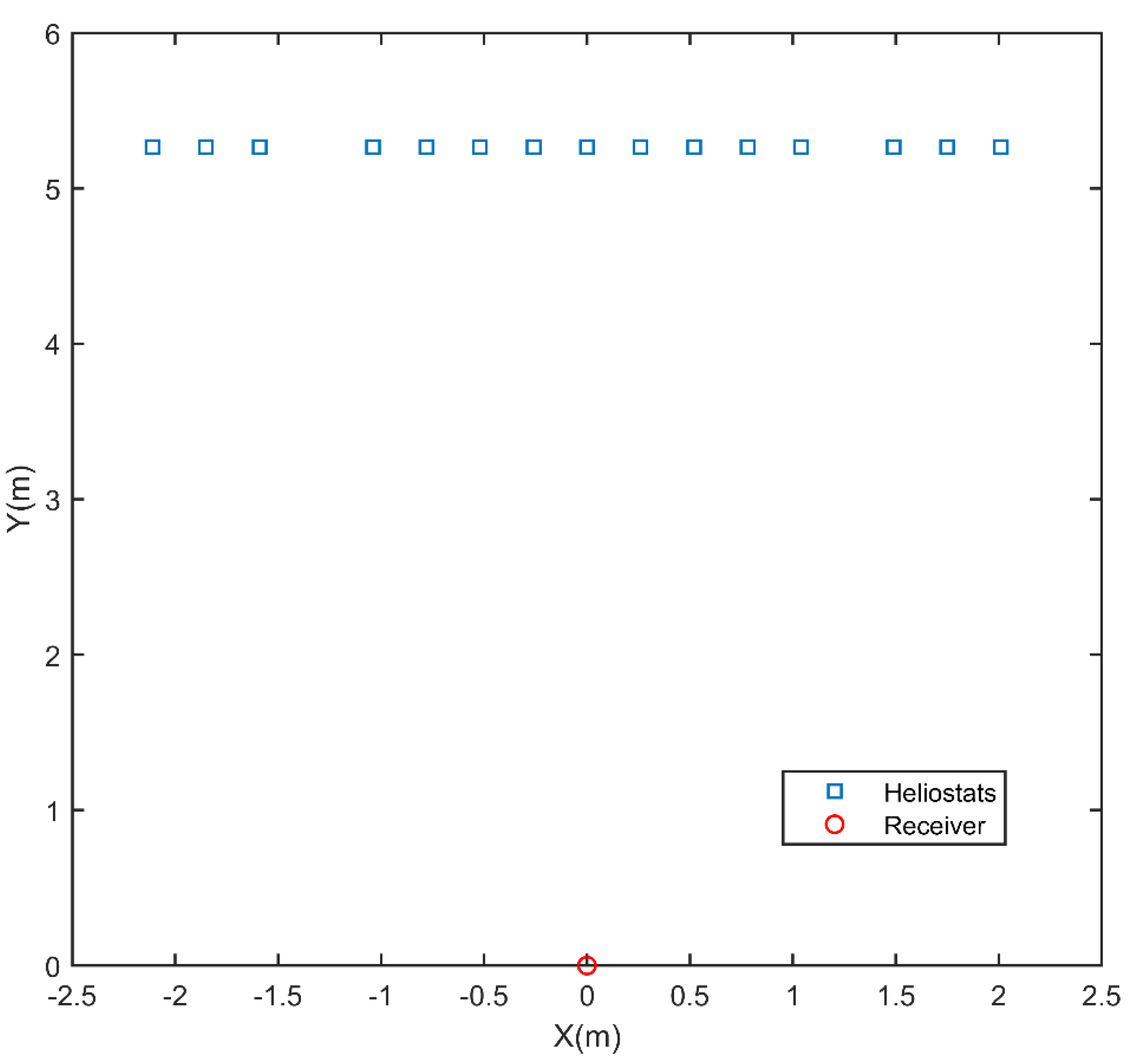
Figure 1. The layout of 15 heliostats.
Sustainability 13 10367 g001
Figure 2. The schematic diagram of the projection.
Sustainability 13 10367 g002
Figure 3. Altitude angle of the Sun: 10°. (a) Solar flux contours which is calculated by SolTrace and the elliptical Gaussian model at the image plane (kW/m2); (b) SolTrace and the elliptical Gaussian model intercepts vs. the side length of a square receiver.
Sustainability 13 10367 g003
Figure 4. Altitude angle of the Sun: 20°. (a) Solar flux Contours which is calculated by SolTrace and the elliptical Gaussian model at the image plane (kW/m2); (b) SolTrace and the elliptical Gaussian model intercepts vs. the side length of a square receiver.
Sustainability 13 10367 g004
Figure 5. Altitude angle of the Sun: 30°. (a) Solar flux Contours which is calculated by SolTrace and the elliptical Gaussian model at the image plane (kW/m2); (b) SolTrace and the elliptical Gaussian model intercepts vs. the side length of a square receiver.
Sustainability 13 10367 g005
Figure 6. Altitude angle of the Sun: 45°. (a) Solar flux Contours which is calculated by SolTrace and the elliptical Gaussian model at the image plane (kW/m2); (b) SolTrace and the elliptical Gaussian model intercepts vs. the side length of a square receiver.
Sustainability 13 10367 g006
Figure 7. Altitude angle of the Sun: 60°. (a) Solar flux Contours which is calculated by SolTrace and the elliptical Gaussian model at the image plane (kW/m2); (b) SolTrace and the elliptical Gaussian model intercepts vs. the side length of a square receiver.
Sustainability 13 10367 g007
Figure 8. Altitude angle of the Sun: 75°. (a) Solar flux Contours which is calculated by SolTrace and the elliptical Gaussian model at the image plane (kW/m2); (b) SolTrace and the elliptical Gaussian model intercepts vs. the side length of a square receiver.
Sustainability 13 10367 g008
Figure 9. CPU time for different number of rays. (Heliostat #1).
Sustainability 13 10367 g009
Table 1. The parameters of heliostats.
#X(m)Y(m)Z(m)Focal Length (m)Length and Width (m)
12.015.265905.90.25 × 0.25
21.755.265905.90.25 × 0.25
31.495.265905.90.25 × 0.25
41.045.265905.90.25 × 0.25
50.785.265905.90.25 × 0.25
60.525.265905.90.25 × 0.25
70.265.265905.90.25 × 0.25
805.265905.90.25 × 0.25
9−0.265.265905.90.25 × 0.25
10−0.525.265905.90.25 × 0.25
11−0.785.265905.90.25 × 0.25
12−1.045.265905.90.25 × 0.25
13−1.595.265905.90.25 × 0.25
14−1.855.265905.90.25 × 0.25
15−2.115.265905.90.25 × 0.25
Table 2. The flux density function expression and the calculation equations of main parameters for rectangular heliostats.
Gaussian ModelFlux Density FunctionThe Calculation Equations of Main Parameters
Elliptical
(for rectangular heliostats)
F ( x , y ) = A m I 0 2 π D 2 σ x σ y e x p [ 1 2 D 2 ( x 2 σ x 2 + y 2 σ y 2 ) ] σ x 2 = σ s u n 2 + σ ¯ s x 2 + 4 σ t r x 2 + σ i x 2 σ y 2 = σ s u n 2 + σ ¯ s y 2 + 4 σ t r y 2 + σ i y 2
Table 3. The parameters of the Sun and heliostats.
Incident Light IntensityReflectivityσsunσslopex,yσtrk
1 kW/m212 mrad1 mard0
Table 4. The average absolute difference of flux density and intercept factor.
Altitude Angle of the Sun10°20°30°45°60°75°
Flux density0.56%0.46%0.45%0.64%0.80%3.54%
Intercept0.26%0.23%0.22%0.32%0.70%3.12%
Publisher’s Note: MDPI stays neutral with regard to jurisdictional claims in published maps and institutional affiliations.

