UAV Based Spatiotemporal Analysis of the 2019–2020 New South Wales Bushfires

Abstract

Bushfires have been a key concern for countries such as Australia for a long time. These must be mitigated to eradicate the associated harmful effects on the climate and to have a sustainable and healthy environment for wildlife. The current study investigates the 2019–2020 bushfires in New South Wales (NSW) Australia. The bush fires are mapped using Geographical Information Systems (GIS) and remote sensing, the hotpots are monitored, and damage is assessed. Further, an Unmanned Aerial Vehicles (UAV)-based bushfire mitigation framework is presented where the bushfires can be mapped and monitored instantly using UAV swarms. For the GIS and remote sensing, datasets of the Australian Bureau of Meteorology and VIIRS fire data products are used, whereas the paths of UAVs are optimized using the Particle Swarm Optimization (PSO) algorithm. The mapping results of 2019–2020 NSW bushfires show that 50% of the national parks of NSW were impacted by the fires, resulting in damage to 2.5 million hectares of land. The fires are highly clustered towards the north and southeastern cities of NSW and its border region with Victoria. The hotspots are in the Deua, Kosciu Sako, Wollemi, and Yengo National Parks. The current study is the first step towards addressing a key issue of bushfire disasters, in the Australian context, that can be adopted by its Rural Fire Service (RFS), before the next fire season, to instantly map, assess, and subsequently mitigate the bushfire disasters. This will help move towards a smart and sustainable environment.

1. Introduction and Background

Disasters around the globe have been impacting the global economies since the dawn of time. These disasters include earthquakes, floods, hurricanes, tornados, landslides, tsunamis, bushfires, and others [1]. Disasters result in the loss of lives, properties, real estate, and livestock, with serious consequences for the economic development of the affected countries. Accordingly, critical infrastructure, communications, real estate, vegetation, and forests are lost, in addition to the lives that hinder regional development. The reason behind frequent and recurring fire seasons is attributed to climate change [2,3,4]. Climate change, deforestation, growing urban development, and utilization of combustible sources are increasing the global temperatures in countries around the world. This gives rise to bushfires and extreme weather [5]. Consequently, the global fire seasons are getting prolonged, and the daily temperatures are rising, which are predicted to worsen and be more severe if climate change issues are not addressed [6,7]. In the era of demands for global sustainability, it is imperative to address such climate issues.

Globally, bushfires and wildfires burn approx. 4% of the global land surface each year, which amounts to approx. 30–46 million km² of the global land surface [8]. However, due to its limited direct impact on individuals, it does not attract wider attention from the media that is sometimes more focused on reporting only the tragic impacts of such fires that directly impact human lives. As a result, these fires sometimes go unnoticed by the world and are only discussed and addressed in the affected country. In the last two decades, extreme bushfire incidents have been observed worldwide, causing immense economic, social, and environmental loss. The trend of these fires is increasing, and in recent years, this natural disaster has been experienced in the regions where the fires are an unusual event. These include Brazil, Bolivia, Chile, Sweden, and the Arctic Circle [9,10].

In Australia, bushfires are a frequent phenomenon due to their geographic location, varying temperatures, and other natural causes [5]. The deadliest fires in Australian history occurred in 1851, 1939, 1983, 2009, and recently in 2019–2020. As per the report of conversation.com.au, the costs of bushfires have passed $100 billion in Australia, making it the costliest natural disaster [11]. Australia’s 2019–2020 bushfire season, known as the Black Summer Fires, is regarded as one of the worst bushfire events in the country’s history that had serious impacts on wildlife, forests, agricultural land, and public properties. It impacted infrastructure in the states of New South Wales (NSW), Victoria, Queensland, and others. The Black Saturday fires alone burnt 430,000 hectares of land. Overall, the Black Summer fires burnt 10.7 million hectares, equivalent to an area of the size of South Korea or Scotland and Wales combined.

Further, more than a billion wildlife animals have been killed, and over 2000 homes were destroyed due to these bushfires [12]. The major causes of the 2019–2020 bushfires included the extended drought conditions, which left dry bushlands and forests that acted as extremely dry and spatially contiguous fuel spreading through forested regions of NSW stretching from Queensland to Victoria. Several large-scale climate drivers contributed to this dryness of 2019 summer, including a strong and long-lived positive Indian Ocean Dipole and negative Southern Annular Mode. Further, the dryness of the landscape was also influenced by reduced cool-season rainfall and other long-term climate trends. Due to extreme fires, it was challenging to quickly detect and extinguish new ignitions in remote areas where they started, resulting in delayed responses that fuelled the intensity of existing fires and strained the resources. Further, the intensified and dense smoke, due to multiple fire events, made it impossible to know where the fire edge was with precision because line scanner aircraft could not fly, and alternate infra-red scanning was a low resolution or unavailable. These issues made the firefighting more difficult, and the fires grew out of control. The limited capacity to fight fires at night led to many fires taking big runs at night and early mornings, causing havoc in the Australian states of NSW, Victoria, and their border regions [13].

NSW is selected as the study area due to its history of bushfire events. It experiences frequent fires due to its widespread vegetation and bushes that fuel draughts and extreme temperatures.

Table 1. Major bushfires in New South Wales from 1965 to 2020.

Sr.	Year	Fire Events	Area (Hectares)	Deaths	Property Damage	Sources
1.	1965	Southern Highlands Bushfire	251,000	3	59 homes	[14]
3.	1980	Waterfall Bushfires	1,000,000	5	14 homes	[16]
4.	1984–1985	NSW Fire season	3,500,000	5	0 homes, 40,000 livestock, and $40 million economic damage	[15]
5.	1994	Eastern seaboard fires	400,000	4	225 homes	[17]
6.	2002	Black Christmas bushfires	753,314	0	121 homes	[18]
7.	2006	Jail Break Inn Fire, Junee	30,000	0	7 homes, 4 non-residential buildings	[19]
8.	2006	Pulletop bushfire, Wagga Wagga	9000	0	2 homes, 2500 livestock, 3 vehicles, 50 km of fencing	[20]
9.	2006–2007	Australian Bushfire season	1,360,000	8	83 homes, 20 non-residential buildings	[21]
10.	2013	Warrumbungle	54,000	0	53 homes, 118 other buildings, Agricultural equipment, and infrastructure at Siding Spring Observatory	[22]
11.	2013	2013-NSW fires	100,000	1	208 homes, 40 non-residential homes	[23]
12.	2017	Wentworth falls Winter Fire	52,000	0	35 homes	[24]
13.	2019–2020	Black Summer	1,700,000	33	2439 homes, more than billion wild animals lost	[13]

shows some of the impactful fire seasons in NSW since 1965. In 1965, NSW observed 251,000 hectares of damage, damaging 59 homes, and causing three fatalities [14]. In the 1984–85 fire season, much of the damage was experienced in the loss of livestock and $40 million economic loss [15]. Similarly, in 2013, the Warrumbungle fires impacted 53 houses, 118 buildings, and damaged agricultural infrastructure and buildings. The 2017 Wentworth falls winter fires damaged an area of 52,000 hectares and destroyed 35 homes. The statistics signify that, though the human loss due to these fires in the past had been low, the property and economic loss had been severe in each fire event. Further, in the growing era of sustainability and wildlife protections, it is imperative to devise plans that reduce the impacts of such fires on global climate, wildlife, and public properties. Nevertheless, the latest fires associated with the Black Summer event had been tragic in all aspects for the state of NSW and Australia in general. These have resulted in the loss of 33 lives, 10.7 million hectares of land burnt, more than 2400 homes destroyed, and more than a billion wild animals lost [13].

The state of NSW used several remote sensing techniques during the 2019–2020 fire seasons to assess the fire damages. Fire and land management agencies at state and federal levels have remote sensing capabilities that provided useful information during the planning, preparation, and response phases of the 2019–2020 bushfire season. NSW rural fire service (RFS) uses remote sensing technologies in various ways. In a report, NSW RFS reported that its firefighters on the ground and in vehicles provided the best intelligence they could on fires, considering the extent and scale of the fires. Further, it found camera platforms on helicopters with infra-red and high-definition imagery useful. Further remote sensing data from multispectral scanning devices (‘line scanners’) mounted on contracted fixed-wing aircraft was particularly helpful in assessing bushfire movements, spread, and damages [25]. The NSW RFS reports that, across 165 days during the 2019–2020 season, a total of 565-line scanning flights were flown, amounting to 7469 flight hours.

Another high potential solution to addressing the Australian bushfires emergencies is UAV usage that does not rely on human pilots and has very little potential for data losses. UAVs have been used in various fields such as smart cities, real estate, property management, healthcare, construction, agriculture, and others [26,27,28,29,30,31,32]. These have been extensively explored in addressing disaster situations such as emergency evacuation path planning, flood response, and others [33,34,35,36].

Given that they do not require the presence of human resources, such vehicles can be readily made available to use in case of emergencies such as bushfires. UAVs are thus ideal tools that have been used in a post-disaster scenario. For example, in March 2015, when Tropical Cyclone Pam, a category 5 storm, struck Vanuatu, UAVs were employed for mapping areas to assess the damage [37]. Similarly, when Typhoon Haiyan affected Philippines in November 2013, UAVs were used for aerial imaging to get real-time information on the disaster with the help of aerial imaging and the development of future frameworks for emergency response planning [38]. In a recent study, these have been proposed to be used for bushfires in Victoria Australia [5].

Owing to the nature of the frequently occurring bushfires in Australia and NSW, the current study aims to develop a novel framework for assessing the bushfires and applies UAV swarm knowledge for better decision-making and pertinent hazard mitigation strategies. It uses a geographical information system (GIS) based assessments of the fire hot spots of NSW. Further, an unmanned aerial vehicle (UAV) based framework is presented to monitor the bushfire hotspots and instigate immediate rescue measures for minimizing the impacts of these bushfires. The paths of the UAVs are optimized for effective monitoring of the affected areas with the potential to deliver any information, ration, or first aid kits. Specifically, the PSO model, available at https://www.mathworks.com/matlabcentral/fileexchange/69027-simulation-of-particles-in-particle-swarm-optimization (accesed on 9 August 2021) has been used in the study as a base model that has been considerably modified and expanded to suit the needs of the current study.

The rest of the paper is organized as follows. Section 2 presents the potential tools and techniques to help bushfires management. These include the GIS and remote sensing tools and UAVs. Section 3 presents a comprehensive overview of the methodology of the current study and lists key assumptions, constraints, and model codes used in the study for UAV routing problems. Section 4 discusses the key results of the GIS-based assessment of the fire hotspots and the routing results for UAV path planning. Finally, Section 5 concludes the study and presents the future directions to build upon the current study.

2. Potential Tools and Techniques for Bushfires Management

Satellite data obtained through GIS and remote sensing is a widely used primary source of information for the active mapping of fire and burned areas at regional to global scales. The Moderate-resolution Imaging Spectroradiometer (MODIS) from NASA Terra and Aqua satellites were the first satellite-borne sensors with the ability of monitoring fire radiative energy (FRE) release rate, or power (FRP), quantitatively on a worldwide scale. Researchers around the globe have used these to assess wildfires [39,40]. Two kinds of satellite data are used to detect fire events: active fire and burned area products [41]. Burned area products are based on the variations in the reflectance or with the combination of reflectance and active fires [42,43]. In comparison, active fire products are dependent on the detection of thermal anomalies [44].

The GIS tools that enable the monitoring of bush fire hotspots are kernel density and Getis-Ord Gi* hotspot analysis. The kernel is a widely used estimator that helps generalize or smoothen discrete point data into a continuous surface area [45]. On the contrary, Getis-Ord uses the Gi* statistics to calculate the degree of correlation of weighted features in the specific distance threshold. It can be used to identify the clustering pattern in the study area [46,47]. Gi* statistics benefit from concurrently capturing the frequency of the events, the corresponding values, and the spatial relationship [46]. These simple yet efficient GIS tools have extensive applications as spatial, such as and cluster analysis tools in bushfire hazard management. Accordingly, remotely sensed data coupled with GIS tools could facilitate the local administrations to reduce natural disasters such as bushfires [42].

In NSW, remote sensing is an invaluable aid in predicting the weather, climate and assessing fire location. It has been used to assess fire conditions, extent, and behaviour by the NSW Rural Fire Service (RFS) in the 2019–2020 bushfire season. However, Australia’s capabilities in this field have not been harnessed to fight bushfires swiftly and properly. Currently, these tools are only used after a fire is initiated due to a lack of automation and implementation in Australian contexts. Remote sensing must be properly adopted for automatic sensing of fire for big fire-risk seasons. The positive points are that Australia has developed infrastructure and defence agencies that are already using remote sensing techniques, which can be shared with other departments for bushfire management. The key improvement areas include the enhanced capability for early detection of new ignitions, real-time tracking of the fire edge progression and intensity as it spreads, and a better understanding of vegetation and fuel load issues before the fires start. Such remote sensing can monitor and analyse the causal factors of a bush fire, inform the planning department to prepare for, and promptly respond to a bushfire event. Accordingly, a spatial technology acceleration program is needed in NSW (and Australia) to maximize the information available from all the various remote sensing technologies currently used.

For 214 days, from 10 August 2019 to 11 March 2020, NSW RFS flew its line scanning aircraft for at least some time on 88% of days. These line scanning techniques produce good quality imagery above active bush fires, making it possible to see details of the fire edge, its extent, and intensity. Such imagery helped NSW RFS make informed decisions about resource commitments and public warnings during fire events at the height of the 2019–2020 bushfire season. Not downplaying the efforts of the NSW RFS, the destruction levels are still well above the acceptable levels, and the techniques must be revised and improved to minimize the level of destruction. Accordingly, more line scanning and remote sensing techniques can help improve disaster response. Given the relatively low number of aircraft available, and the number of large fires raging simultaneously, only a relatively small number of line scanner ‘snapshots’ of each fire had been possible in the Black Summer. This is a serious drawback given the highly dynamic and dangerous nature of these fires. Further, a drawback of any sensor mounted on piloted, fixed-wing aircraft is that the sensor is useless when the plane cannot fly, as smoke/dust/fog makes flying impossible. The NSW RFS estimates that there were 26 days between 10 August 2019 and 11 March 2020 when line scanning aircraft could not be used at all due to ambient conditions affecting visibility or resourcing considerations. It is important to note that these figures do not include instances where scanned imagery was insufficient or where scans could not be completed frequently. While this is a relatively small period (12%), this inability to fly can be an issue when information about new ignitions, edges, and spread is needed instantly. Thus, it is imperative to explore new techniques and improve the existing ones for better bushfire management. A candidate for this is the usage of a UAV.

UAVs have been used in bushfires assessment, in bushfire hotspot detection [48], and economic evaluation of wildfires through UAVs [49]. Similarly, conceptual discussions have been retrieved from literature as relevant to fire monitoring with UAVs through cognitive human-machine interfaces and interactions [50], as well as remote sensing, to assess grapevine canopy damage due to fire smoke [51] and improve readiness for the next major bushfire emergency [52]. In the case of Australia, these have been proposed to assess bushfires in the state of Victoria [5].

Different types of algorithms exist for planning and optimizing UAV paths efficiently and effectively to reduce associated costs. These include Java-based algorithms, such as greedy, inter-route, intra-route, Tabu, and particle swarm optimization (PSO) [53,54]. Other studies have used Ant Colony Optimization (ACO) and Genetic Algorithm (GA) techniques. However, PSO has never been used for path planning of UAVs for bushfire assessment in NSW Australia, which is a humble contribution of the current study. PSO is a heuristic method that starts its search process using an initial particle population [55,56,57]. Each particle represents a potential solution to the problem [58]. There is a multi-dimensional search space where these particles move around until they reach a constant state or the computational constraints are fully exhausted. PSO mimics the behaviour of birds in a flock or sheep in a herd [59]. It is based on a collection of particles in a swarm where each particle represents a possible solution to the problem. Due to its established advantages, PSO has been utilized in the current study, taking advantage of its ease of implementation, few parameters to adjust, robust, higher efficiency in finding the global optima, converge quicker, short computational time, and no overlapping.

A comprehensive, optimized UAV system has not been proposed, to date, in the relevant literature for assessing bushfires issues and subsequent management in the Australian context. This gap is targeted in the current study, where the applications of UAVs are proposed and tested in the NSW region of Australia that is prone to frequent bushfires. Overall, the current study uses a mix of remote sensing and GIS for bushfire hotspot assessments and develops a UAV based optimized path system for instigating a swift emergency response to help mitigate bushfire disasters. Burnt locations and hotspots of 2019–2020 bushfire season in the NSW are assessed using GIS tools and remote sensing data of VIIRS. Further, the statistical significance of these fire events, using the geostatistical tool of Getis Ord Gi* statistics, is also assessed to discuss the impact of damage by the 2019–2020 fires.

3. Materials and Methods

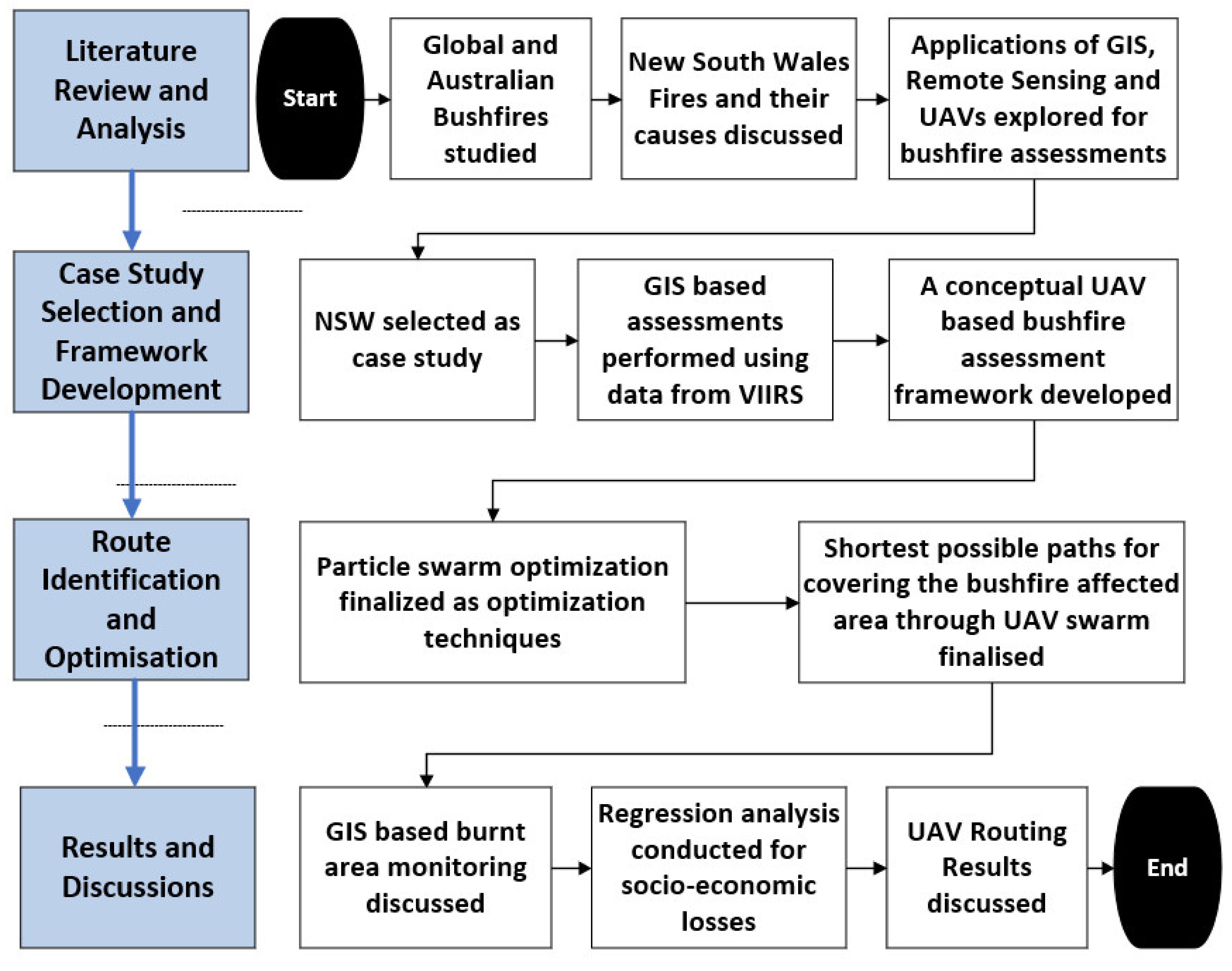
This study follows a systematic approach for addressing the bushfires disasters in NSW regions of Australia. A four stepped method is adopted in the current study, as shown in Figure 1. In the first step, a review of the data available about global and Australian bushfires is conducted, as evident from the introduction section of the current study. This is augmented with the data about fires in NSW. Afterward, GIS, remote sensing applications, and UAVs for bushfire assessments are discussed in the section of tools and techniques available for bushfire assessment. In the second step of the current study, GIS-based assessments and burnt area monitoring are performed using data from VIIRS, and a UAV-based bushfire assessment framework is presented. In step three, the paths of UAV swarms are optimized using the PSO algorithm to identify the shortest possible paths for covering the bushfires area. In the fourth and final step of the study, the GIS-based bushfire monitoring reports are presented along with the regression analysis for bushfires-related socio-economic loss assessments. Lastly, the PSO-based UAV optimization results are presented to discuss the best routes for UAVs in mitigating bushfires disasters and instigating a swift response.

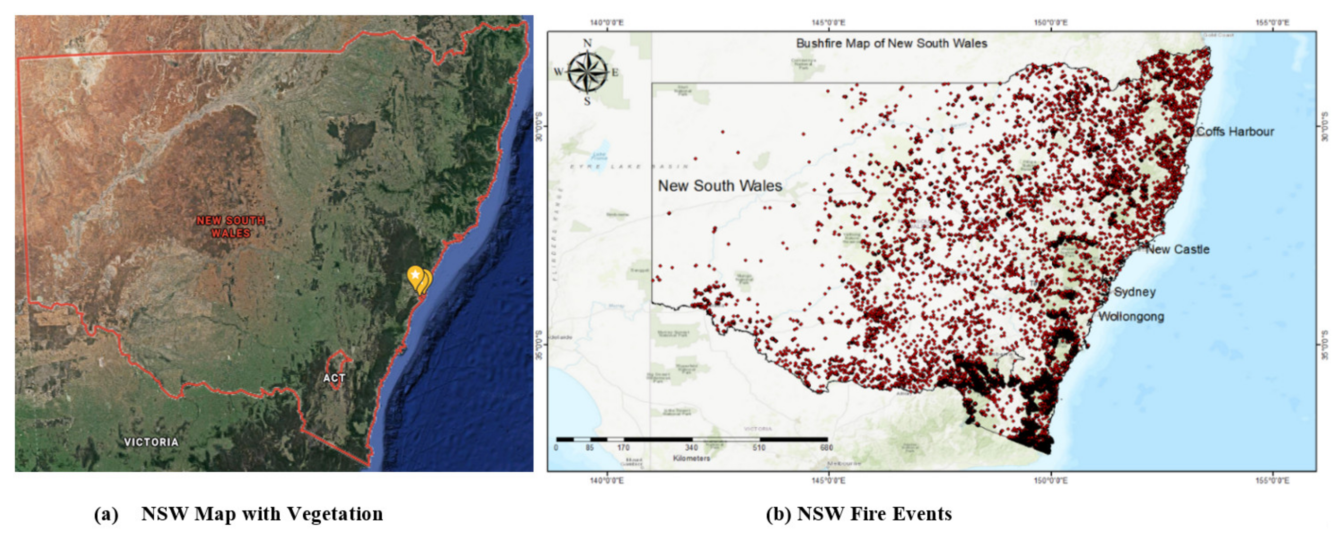
3.1. Study Area

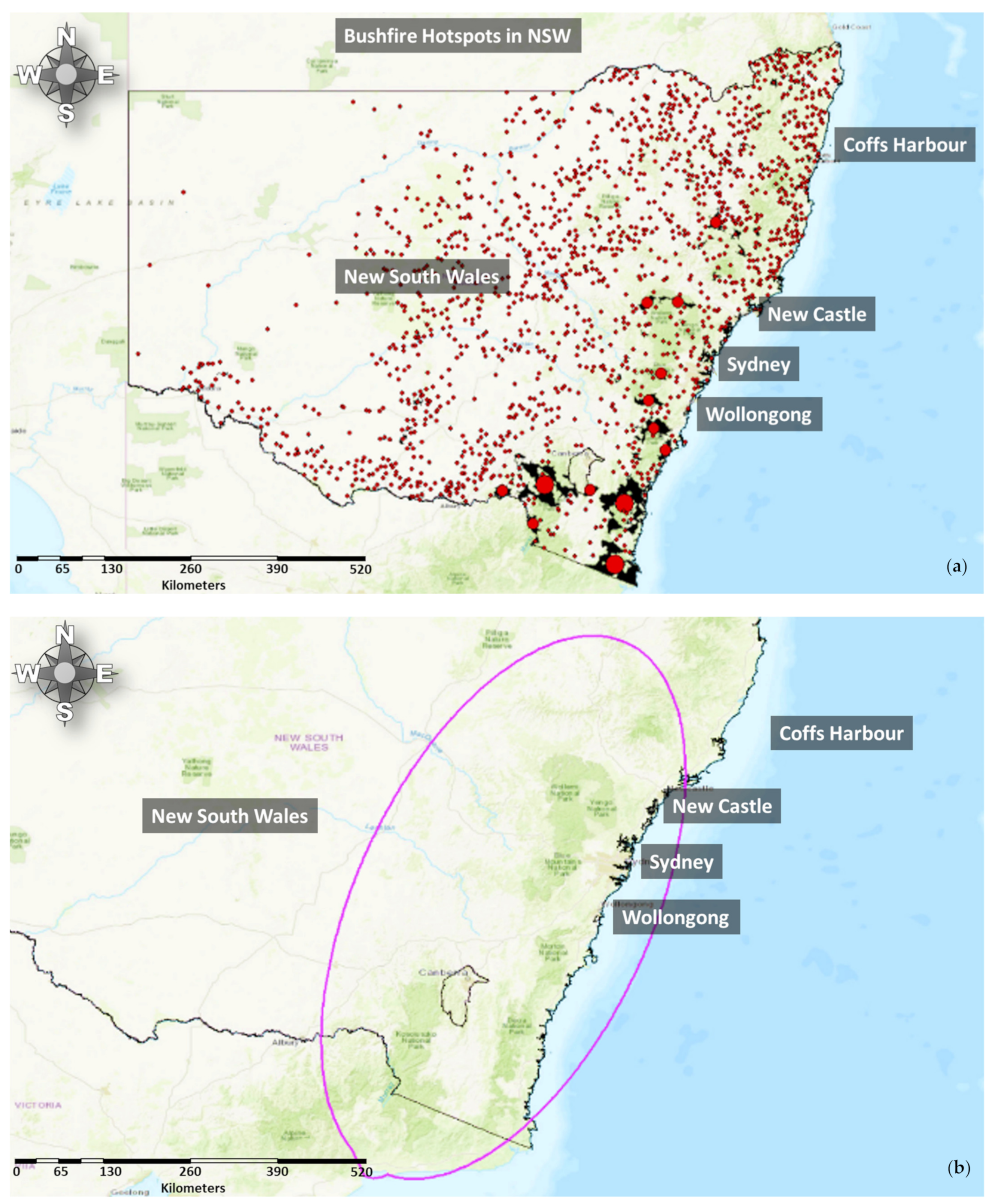
The case study area of the current study is the state of NSW, Australia. The state is in the southeast of Australia on the eastern coast. It houses Sydney, the most populated city in Australia, and is among the top revenue-generating states in Australia. The area of NSW is 801,150 km² and has a population of approx. 8.092 million as of 2020. Vegetation bushlands cover over 80% of NSW and forests, as shown in Figure 2a, making it a frequent bushfire experiencing state. The motivation to choose the NSW for this study is that the state was set ablaze in the recent Black Summer fires and has reported the highest loss among all Australian states. The state observed 10,520 fire incidents in its various parts, destroying 75% of the total infrastructure losses of the Black Summer fires. Figure 2b provides the total fire events for NSW, based on GIS and remoting sensing, using the data from VIIRS sensors.

3.2. Study Datasets

Table 2. The datasets used for the study.

Data	Type	Date of Acquisition	Source
Fire points	VIIRS	14 October 2020	Fire Information for Resource Management System (FIRMS)
Temperature	Mean Temperature Deciles	14 October 2020	Australian Government Bureau of Meteorology
Rainfall	Rainfall Deciles	14 October 2020	Australian Government Bureau of Meteorology
Forest Fire Danger Index (FFDI)	FFDI Deciles	14 October 2020	Australian Government Bureau of Meteorology

summarizes the dataset used in the study. The primary dataset used for this study is the National Oceanic and Atmospheric Administration (NOAA) data of the VIIRS fire product. The VIIRS empowers operational environmental monitoring and numerical weather forecasting. It has 22 imaging and radiometric bands covering wavelengths from 0.41 to 12.5 microns. It provides sensor data records for more than twenty environmental data records such as the clouds, sea surface temperature, ocean colour, polar wind, vegetation fraction, aerosol, fire, snow and ice, vegetation, etc. The on-orbit verification in the postlaunch check-out and intensive calibration and validation have shown that VIIRS is performing very well. It has been used in the current study due to its precise resolution of detecting the smallest fires. The VIIRS sensor identified 10,446 fires, including minor and major fires, within NSW for the 2019–2020 Black Summer time. Apart from the fire product, climatic data for mean temperature, mean rainfall, and Forest Fire Danger Index (FFDI) are acquired from the Australian Government Bureau of Meteorology. This data is used to study the underlying climatic conditions responsible for these bushfires. These datasets monitor the burnt area and bushfire hotspots in the NSW region for the Black Summer period.

3.3. GIS Analyses of the NSW Bushfires

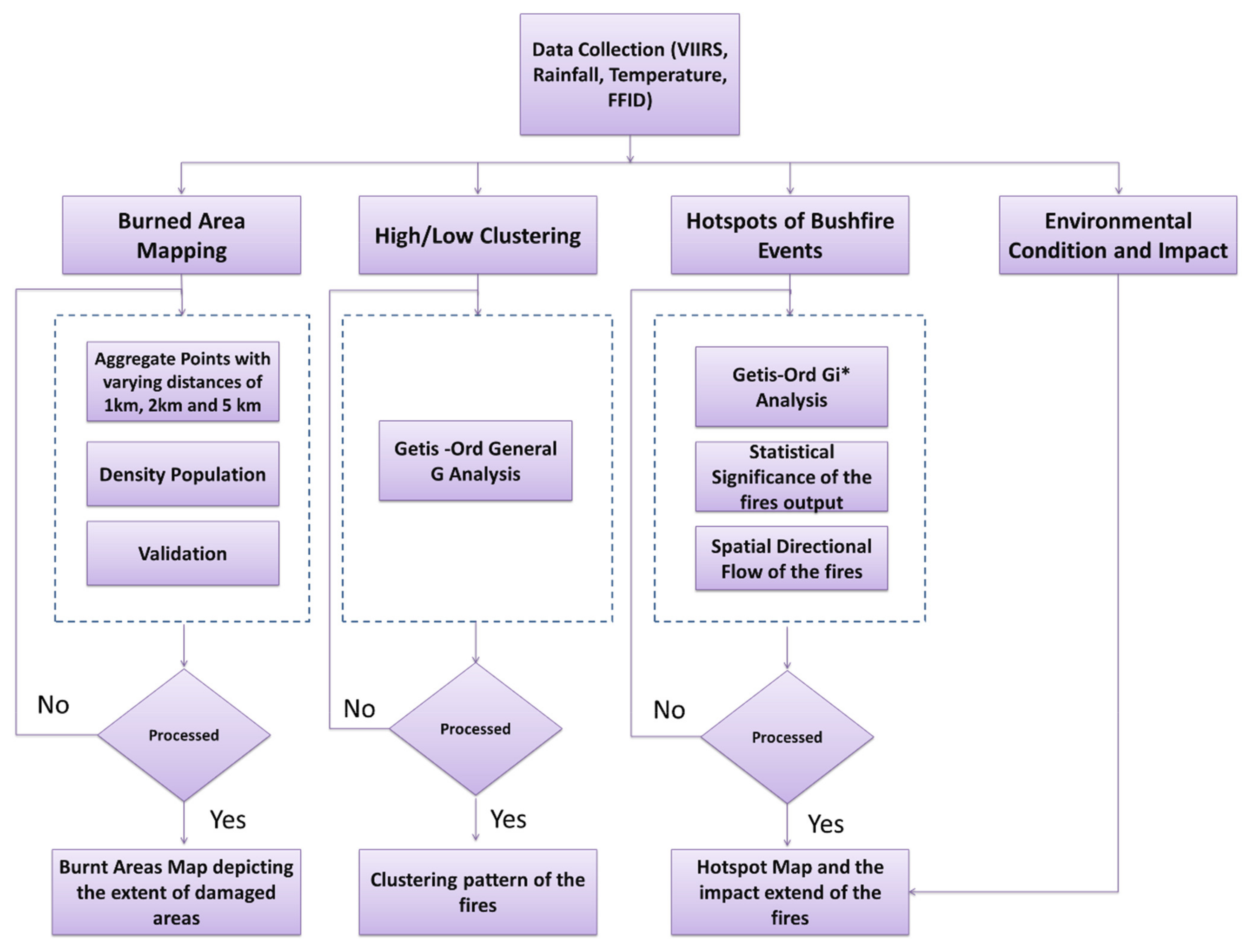
Figure 3 provides the methodology flowchart to monitor the burnt area and map bushfire hotspots in the study area. The data and annual reports, from the Australian Bureau of Meteorology, of the region of interest were acquired. An in-depth review and assessment were used to relate and understand the fire patterns and areas identified in the analysis. Accordingly, four key steps were performed: burned area mapping, fire clustering, hotspot monitoring, and environmental conditions and impact.

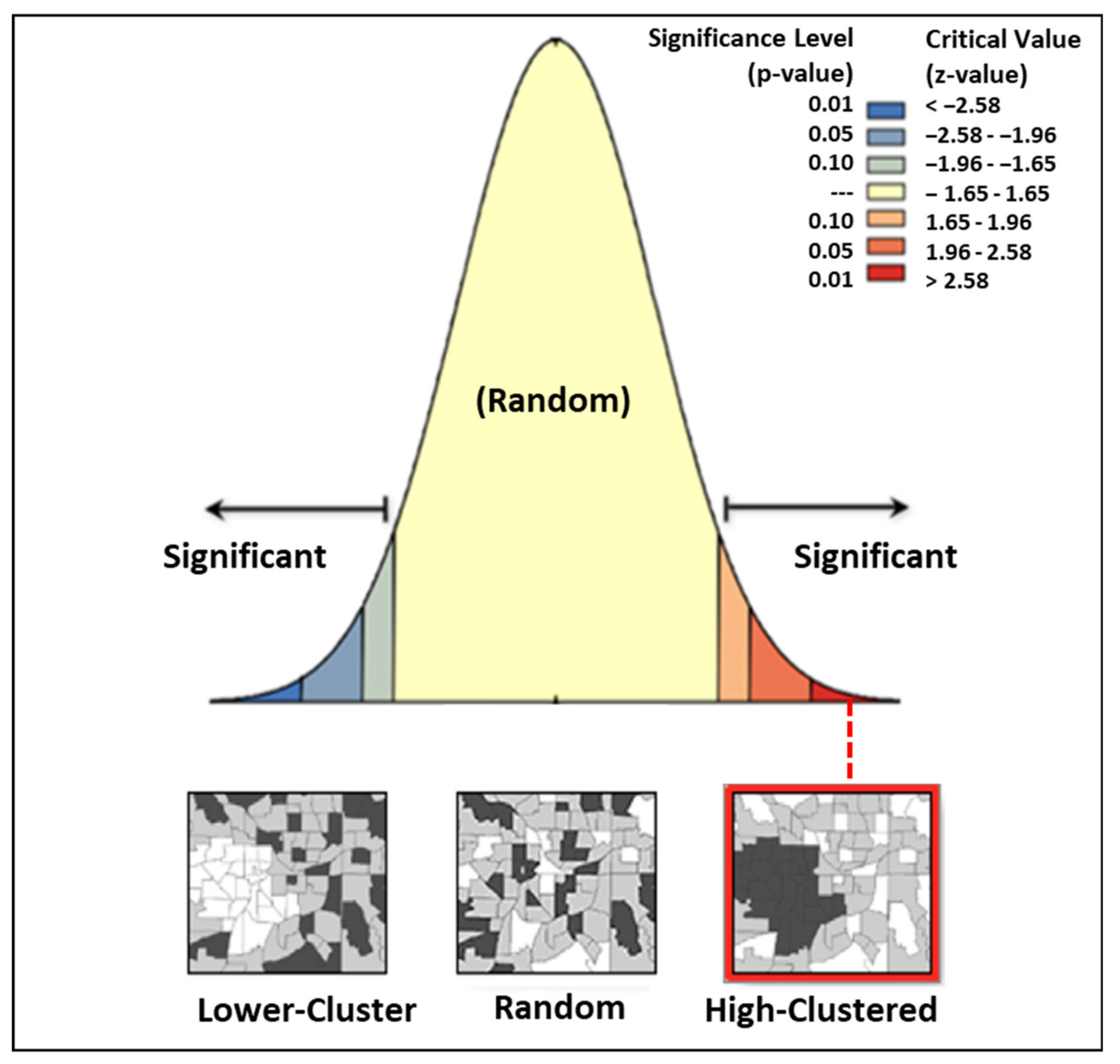
For mapping the burnt area, ArcGIS software is used in which the interpolated perimeters from the monthly accumulated fire points are generated using a convex hull aggregation with the ‘aggregate points’ tool. The convex hull algorithm assigns an area including the clusters of points (minimum 3) at user-defined aggregation distance. Three aggregation distances, 1 km, 2 km, and 5 km, are tested for the fire delineation. These distances are chosen depending on the spatial resolution of the active fire products from the VIIRS-375 m resolution. The idea is to visualize the total burned area due to the fires in the NSW region. The validation of the fire samples is performed using visual interpretation from Google Earth imagery. The High/Low Clustering (Getis-Ord General G) provides the fires’ gathering pattern that is used to measure the extent of clustering in the fire data.

The z-score and p-value depict the statistical significance of the null hypothesis. In this case, the null hypothesis states that the values linked with each feature are distributed randomly. For monitoring the hotspots, Getis-Ord local Gi* spatial statistics is performed to see the statistical significance of the fire incidents. Before the incremental spatial autocorrelation tool is operated, beginning distance and distance increment must be set. Calculate Distance Band from the Neighbor Count tool is used to monitor these parameters. The tool gives the minimum, average, and maximum distance at which each point has at least one neighbour. The resultant maximum distance is used as the beginning distance, whereas the average distance achieved from the tool is used as the distance increment. Later, the incremental spatial autocorrelation tool is used to measure data grouping in space. The tool gives an output in the form of a graph of increasing distances and their corresponding z scores.

The clustering distance is subsequently used in the Getis-Ord Gi* analysis as a distance band or radius. The Getis-Ord local statistic is calculated using Equations (1)–(3).

$$G{i}^{*}=\frac{{{\displaystyle \sum }}_{j=1}^{n}wij.xj-\overline{x}{{\displaystyle \sum }}_{j=1}^{n}wij}{S\sqrt[2]{\frac{\left[n{{\displaystyle \sum }}_{j=1}^{n}w{i}^2.j-{{\displaystyle \sum }}_{j=1}^{n}wij{]}^2\right]}{n-1}}}$$

(1)

$$\overline{x}=\frac{{{\displaystyle \sum }}_{j=1}^{n}xj}{n}$$

(2)

$$S=\sqrt[2]{[n{\displaystyle \sum }_{j=1}^{n}x.j^2-{(\overline{x})}^2}$$

(3)

where xj is the attribute value for feature j, wi.j is the spatial weight between the feature i and j, and n is the number of features. $\overline{x}$ is the mean of all measurements, and S is the standard deviation of all measurements. The Gi* is a zone, after which no more calculations are required. The Gi* statistic returned for the features in the fire datasets is a z-score. For the z-scores to be statistically significant, the higher the z-score value, the more intense the cluster will be, hence classifying it as a hot spot. Consequently, the cluster will have low values for statistically strong negative values, identifying it as a cold spot. Thus, the spots can be classified into hotspots or cold spots for assessing the fires. Lastly, a linear regression analysis is performed, with the response variables of the burned area, fire incidents, fatalities, and the predicting variable as the fire season (year). Positive and negative relationships are represented as increasing and decreasing trends, respectively.

3.4. PSO for UAVs Path Planning in Bushfires Monitoring

PSO is a metaheuristic algorithm that works on the principle of finding, generating, and searching for the shortest path. In this study, the PSO algorithm is used to monitor the bushfire area. It is quite challenging, in bushfires, to reach the allocated area and hover back to the depot. In the relevant literature, compared to the existing algorithms such as ACO and GA, PSO is favoured to generate the shortest distance with enhanced collision avoiding capability [60,61]. Moreover, it is the best possible approach to significantly find the shortest distance in optimum time [62,63]. In the current study, the PSO optimization algorithm used in UAV Bushfire Application is inspired by “Seyedali Mirjalili (2021). 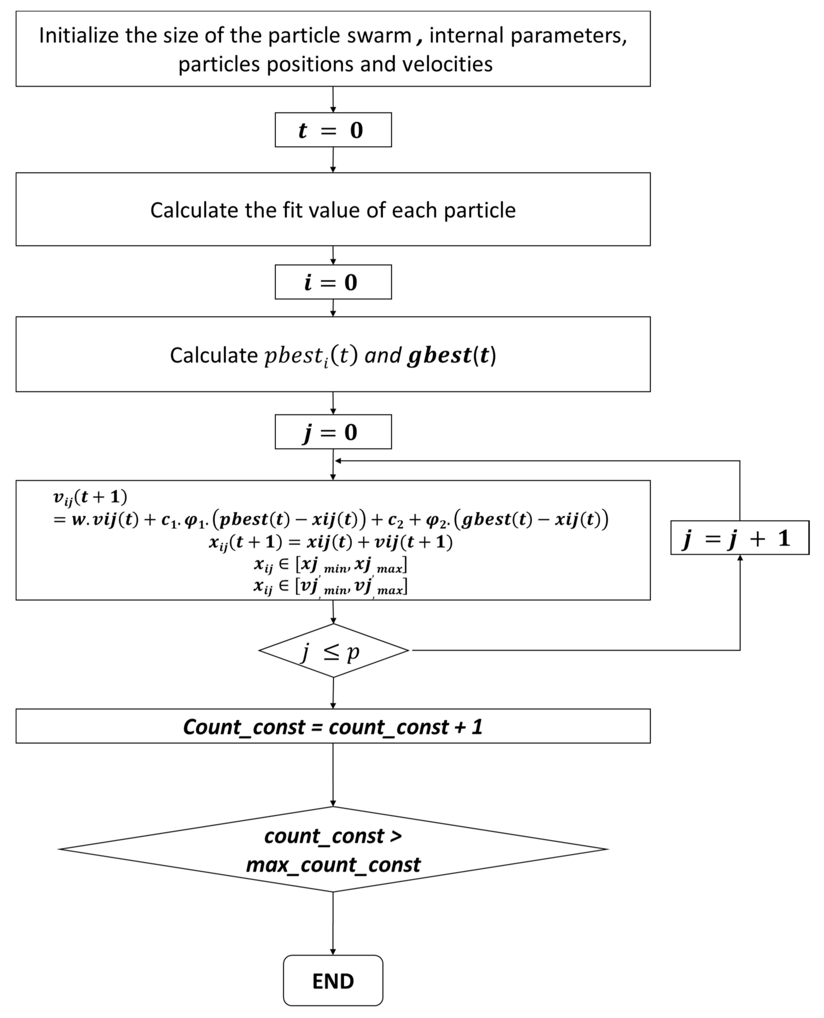Simulation of particles in Particle Swarm Optimization”, available at (https://www.mathworks.com/matlabcentral/fileexchange/69027-simulation-of-particles-in-particle-swarm-optimization, accessed on 9 August 2021). The document was accessed on 9 August 2021. Significant changes have been made to the source code, including changing the parameters, e.g., handle points, maximum iterations, population size, inertial weight, as well as personal and global learning coefficients that have been modified to be used in our specific application where the particles are the UAVs in a swarm. Specifically, three-point handles have been used in the current study compared to the source code. The function used in the current study is for five obstacles with different positions and diameters, which are some of the novel additions and modifications, of the current study, to the source code. Furthermore, based on the computation time and transportation cost, the current study considers the best path for UAVs to reach the affected area in the least time. For this purpose, the number of obstacles has been increased to five to make a complex environment for UAVs to reach the destination.

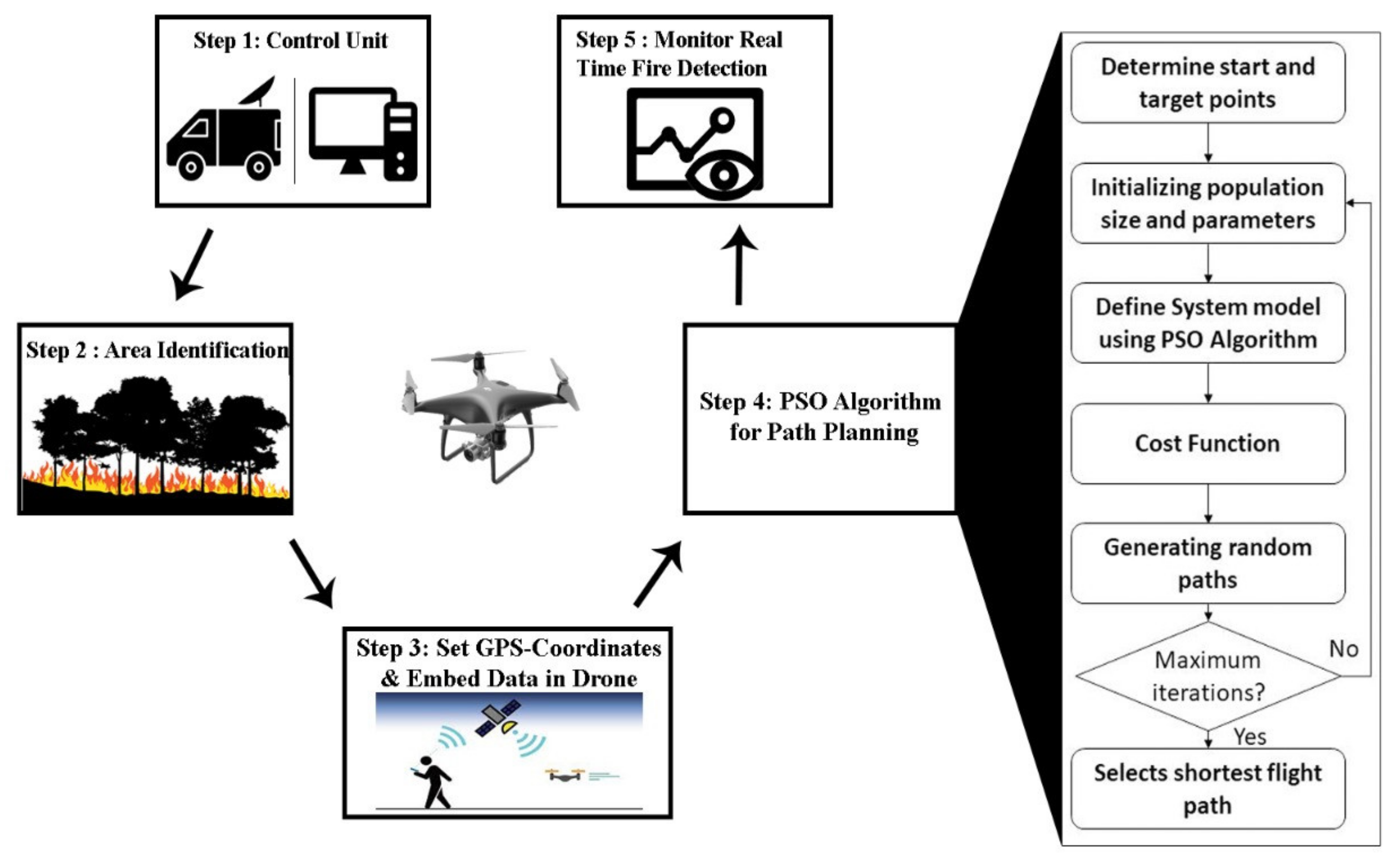
The flow chart in Figure 4 shows the simulation model for the PSO algorithm. Initially, the start and target points are determined for UAVs to fly from the depot (start) and reach the target location. In step 2, the population size and parameters are set for particle velocity, time steps, and personal and global learning coefficient. In step 3, the PSO algorithm model is run to maximize the affected area coverage based on the cost function generated in step 4. As a result, the random paths are generated, and the shortest path is selected based on the maximum iterations.

Figure 5 provides a five-stepped framework for bushfire detection using UAVs through the PSO algorithm. In step 1, the control unit is notified regarding the affected region where the bushfire is ignited using field and satellite sensors. In step two, the control unit/van is sent to the nearest safe area of the bushfire. This is done to avoid unnecessary battery losses of the UAVs due to the hovering of UAVs as they have limited battery power. It further ensures high endurance and better wireless communication with the UAV due to the shorter distance. In step 3, the GPS coordinates of the UAVs are set, and the required data is embedded to cover the targeted location for bushfire damage detection. In step 4, the PSO algorithm is initialized to determine the shortest path between the start point and the end destination, retrieving the data in lesser time and minimum transportation distance. Based on the shortest path calculated, the UAV swarm assigns the task to each other to minimize the energy consumption and better monitoring time. In the final step, the real-time fire is monitored using cameras and sensors attached to the UAV. The data is shared with the control unit in real-time, where it can be shared with all concerned departments. A rescue relief team is notified instantly to reduce the effects of bushfires.

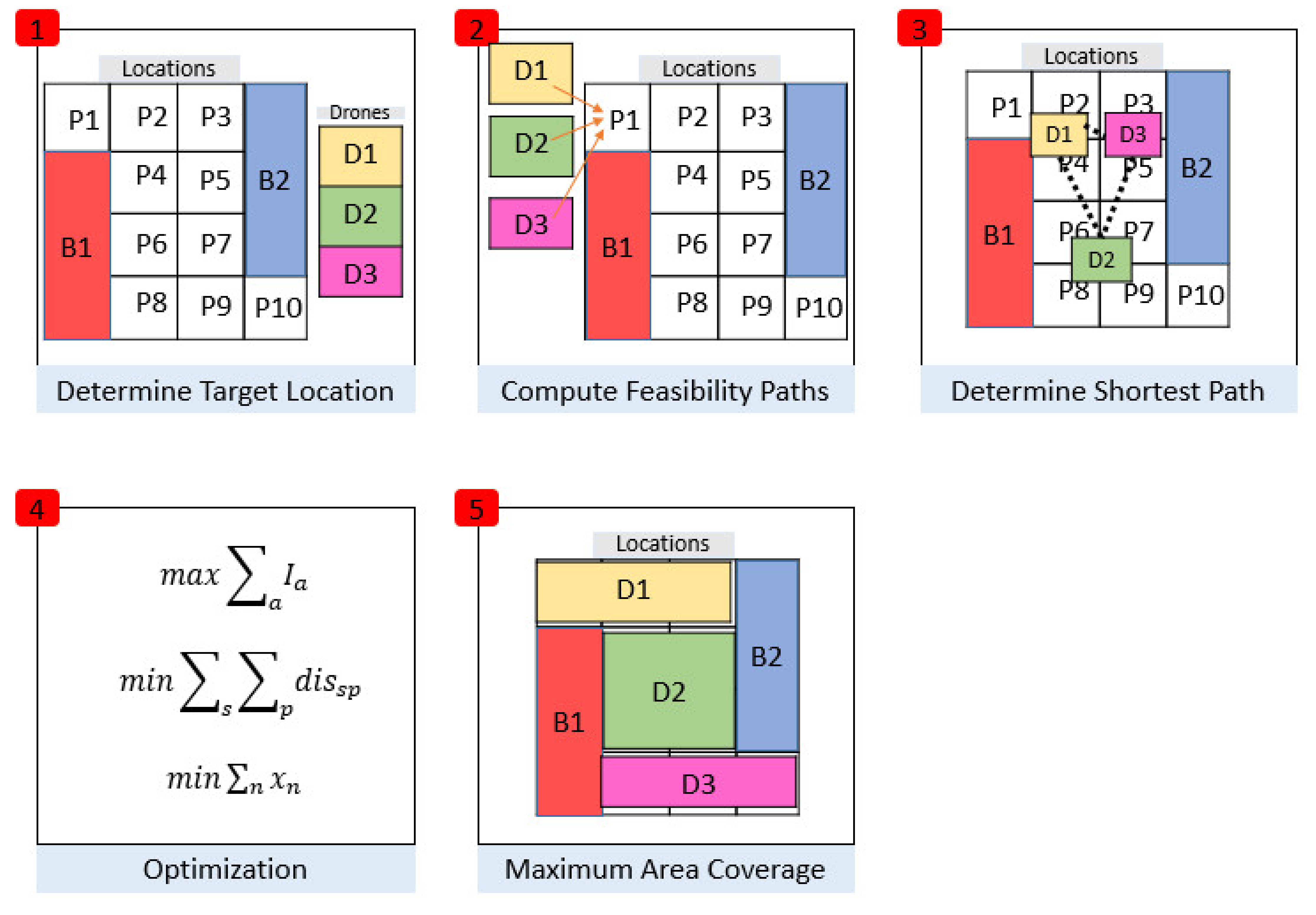
Figure 6 illustrates the pseudocode and demonstrates the trajectory of UAVs from determining the maximum area coverage. In Figure 6, it is assumed that the B1, B2 are the Barriers, UAV1, UAV2, and UAV3 are the UAVs, while P1–P10 are the locations to be covered by the UAVs. The first step involves determining the target location, which is, identifying the fire zone. The UAVs initialize themselves from P1 to compute the feasibility paths in Step 2. These UAVs are launched from the control units or vans present in the vicinity of the fire zone. To minimize the transportation distance, the UAVs communicate with neighbouring UAVs and determine the shortest path possible in Step 3. In Step 4, the optimization method is adopted, where three of the PSO algorithm functions are run to maximize the area coverage, minimize the distance to the target, and minimize the number of active UAVs. As a result, an efficient and cost-effective disaster management strategy is devised whereby the UAVs can cover the maximum area in the shortest possible time, as given in Step 5, and where all the locations from P1 to P10 are covered by the three UAVs using PSO. This way, the barriers in the paths are avoided, as evident from B1 and B2 in Figure 6, and an efficient maximum area coverage strategy is used to get data from the target zone.

The area assignment for UAVs is based on the longitude and latitude coordinates using GPS technology [64,65].

Table 3. The PSO parameters and their values.

Parameter Values
w = 0.8	Inertia Weight
wdamp = 0.96	Inertia Weight Damping Ratio
c1 = 1.25	Personal Learning Coefficient
c2 = 1.25	Global Learning Coefficient

lists the parameters and assumed values of these parameters to assist the PSO algorithm. The inertia weight determines the contribution rate of a particle’s previous velocity to its velocity at the current time step that is considered as 0.8 in the current study. The inertia weight damping ratio is assumed as 0.96. The personal learning coefficients and the global learning coefficients to fit the maximum area curve are 1.25. These values are taken from the studies of Mirjalili et al. [66] and Mirjalili et al. [67] based on the optimum results achieved.

3.5. Proposed Model

The parameters and functions of the proposed model are presented in

Table 4. Model parameters and functions.

Parameters	Functions
D	Set of depot sites
T	Set of target sites
0, n + 1	The start and end depots of the drone
V	V = D $\cup$ T$\cup$ (0) $\cup$ (n + 1)
R	Set of UAVs
qi	Requested demand for each target site $iϵ$ T
qr	Capacity of drone $rϵ$ R
Pr	Time required for UAV to cover area $rϵ$ R
ai. bi	Time window during which the UAV reaches the target site
tij	Time to travel from i to j, $jϵ$ V
r	Maximum time lag between consecutive deliveries

.

The UAV starts its trip at a central (source) depot and travels between the depot and target sites. At the end of mission completion, the UAV returns to an end (sink) depot (which may or may not be the same as the starting depot). This routing problem can be modelled on a directed, weighted graph G (V, A); consisting of vertex set V= {0} ∪ T ∪ {n+ 1}, where vertices 0 and n + 1 are resp. to the source and sink depots. The UAV must reload in between 2 deliveries. This has been accounted for in the arc costs. Optionally, a positive load time for the UAVs can be added to the arcs between two target sites. The arc set A is defined as follows:

• The source-sink depots have outgoing resp. incoming edges to/ from all other vertices.
• There is an arc (i,j) for all i; j ϵ T; i ≠ j.

The arc costs are as follows:

• T_0,i = min_pϵP t_i,p + t_p,j for all i ϵ T
• T_i,j = min_pϵP t_i,p + t_p,j for all i, j ϵ T
• T_i,n+1 = t_i,n+1.
• T_0,n+1 = 0.

The routing constraints can be modified as follows:

$$max. {\displaystyle \sum }_{i \in T}{q}_{i Y_i}$$

(4)

$${\displaystyle \sum }_{r \in R\in \delta +\left(i\right)}.{\displaystyle \sum }_{.}qr Xij\mathrm{R} \ge qiYi \forall i ϵ \mathrm{T}$$

(5)

Constraint (5) ensures that enough area is covered at the target site.

$${\displaystyle \sum }_{j\in \delta +\left(0\right)}X0jr={\displaystyle \sum }_{i ϵ \delta \left(n+1\right)} Xi,n+1,r=1 \forall r ϵ \mathrm{R}$$

(6)

$${\displaystyle \sum }_{j\in \delta +\left(i\right)}Xijr={\displaystyle \sum }_{j ϵ \delta -\left(i\right)} Xj,i,r \forall i ϵ \mathrm{T},r ϵ \mathrm{R}$$

(7)

Constraints (6) and (7) determine the shape of a feasible tour: a tour starts at the source depot, visits a target site, and finally returns to the sink depot. Constraints (7) are the flow preservation constraints. Further, between two consecutive visits, starting, processing, and travel times must be considered (Constraint (8)).

$$T_r^i+t_{ij}-\mathrm{M}\left(1-X_{ijr}\right)\le T_r^j-D_r \forall i, j ϵ \mathrm{V}, r ϵ \mathrm{R}$$

(8)

$$a_{i+}{D}_r\le T_r^j \le b_i \forall i ϵ \mathrm{V}, r ϵ \mathrm{R}$$

(9)

A target i ϵ T cannot be visited before a_i, and the assigned task must be completed before b_i (Constraint (9)). The remaining Constraints (10)–(12) restrict the domains of the variables.

$$X_{ijr} ϵ\left\{0,1\right\} \forall i, j ϵ \mathrm{V}, r ϵ \mathrm{R}$$

(10)

$$T_r^i ϵ\mathrm{Z}\ge 0 \forall i ϵ \mathrm{V}, r ϵ \mathrm{R}$$

(11)

$$Y_i ϵ \left\{0,1\right\} \forall i ϵ \mathrm{T}$$

(12)

where, $X_{ijr}$ is a binary variable, indicating whether UAV r travels from i to j. Integer variable $T_r^i$, i ϵ T, r ϵ R, record the time that UAV r finishes its delivery to target site i. For notation purposes, δ⁻ (.) resp. δ⁺(.) denote the incoming resp. outgoing neighbourhood sets. The maximum time lag requirements between multiple tasks completed for a single site can be schedules as below:

$$max. {\displaystyle \sum }_{i \in T}{q}_{i Y_i}$$

(13)

$${\displaystyle \sum }_{r\in Rl ϵ R0\backslash \left\{r\right\}}.{\displaystyle \sum }_{.} q_r Z_{rl}^l \ge q_{i } Y_{i } \forall i ϵ \mathrm{T}$$

(14)

Constraint (14) ensures that assigned tasks have been completed at each target site.

$${\displaystyle \sum }_{i \in R0}{Z}_{r0l }^i=1 \forall i ϵ \mathrm{V}$$

(15)

Constraints (15) and (16) are used to sequence the UAVs. A UAV can only be used once for every target site, and whenever it is used, its delivery must be succeeded by another delivery (possibly a delivery by the dummy UAV r₀) (Constraint (15)). The dummy UAV must be scheduled (Constraint (16)).

$${\displaystyle \sum }_{l \in R0 \backslash \left\{r\right\}}{Z}_{rl }^i={\displaystyle \sum }_{l \in R0 \backslash \left\{r\right\}}{Z}_{lr }^i \forall r, l ϵ \mathrm{R}, r \ne l, i ϵ \mathrm{V}$$

(16)

Constraint (17) is the flow preservation constraint. Together with Constraint (16), these constraints enforce that all assigned tasks are scheduled consecutively. Thus, each task has exactly one successor and one predecessor.

$$T_r^i-\mathrm{M}\left(1-Z_{rl }^i\right)\le T_{rl}^i-D_l \forall r, l ϵ \mathrm{R}, r \ne l, i ϵ \mathrm{V}$$

(17)

Constraint (17) links the completion time variables $T_r^i$ and the sequence variables $Z_{rl}^i$, thereby enforcing that tasks performed do not overlap in time.

$$T_l^i–D_l\le T_{r }^i+\gamma +\mathrm{M}\left(1-Z_{rl}^i\right) \forall r, l ϵ \mathrm{R}, r \ne l, i ϵ \mathrm{V}$$

(18)

Constraint (18) enforces a maximum lag time between consecutive assigned tasks.

$$a_{i+}{D}_r \le T_r^j\le b_i \forall i ϵ \mathrm{V}, r ϵ \mathrm{R}$$

(19)

Constraint (19) ensures that assigned tasks performed by the UAVs are scheduled within the time window. The remaining Constraints (20)–(22) restrict the domains of the variables.

$$Z_{rl }^iϵ\left\{0,1\right\} \forall i ϵ \mathrm{V}, r, l ϵ \mathrm{R}$$

(20)

$$T_r^i ϵ\mathrm{Z}\ge 0 \forall i ϵ \mathrm{V}, r ϵ \mathrm{R}$$

(21)

$$Y_i ϵ \left\{0,1\right\} \forall i ϵ \mathrm{T}$$

(22)

The binary variable $Z_{rl}^i$ is equal to one if UAV $r ϵ \mathrm{R}$ completes its tasks immediately before UAV $l ϵ \mathrm{R}$ to target site $i ϵ T$; otherwise, the value is zero. In this model, r₀ represents a dummy drone, R₀ = R U {r₀}. A feasible solution is obtained at the intersection of the routing and scheduling polytopes. Connecting the two polytopes is accomplished via the linking constraints:

$${\displaystyle \sum }_{l ϵR0 \backslash \left\{r\right\}}{Z}_{rl }^i={\displaystyle \sum }_{j ϵ N }{X}_{ijr} \forall r ϵ \mathrm{R}, i ϵ \mathrm{T}$$

(23)

Note that Constraints (14) and (17) in the route are identical to Constraints (5) and (9) in the schedule, respectively, and are consequently dropped.

A disadvantage of the current model is that a single UAV cannot visit the same target site more than once. This restriction is unrealistic as, often, a UAV can travel back and forth between the depot and a target site. When the binary variables $X_{ijr}$ are replaced by equivalent integer variables, indicating the number of times UAV R travels from i to j, one can still distinguish the routes. However, expressing the scheduling constraints becomes difficult in this case. Two options exist to address this issue: either the distinct trips made by a single UAV are enumerated (e.g., UAV R travels from i to j during trip t), or the visits to a target site are enumerated. The latter solution is applied in assignment-based formulations for scheduling problems. This model is adjusted to our notation as below:

Let D and T be defined as above. In addition, for each target site $i ϵ \mathrm{T}$, a new ordered set consisting of visits to the target site, $T^i$ = {1…..n(i)}, is defined where n(i) = [$q_i$/$\underset{r ϵR}{\min }\left(qr\right)$] is an upper bound of visits required by the target site i. A shorthand notation, $t_j^i$ will be used to denote visit j for target i. A time window [$a_e$, $b_e$] is associated with each visit e$ϵ$ $T^i$, $i ϵ \mathrm{T}$ which is initialized to the time window for the corresponding site $i ϵ \mathrm{T}$ i.e., [$a_e$, $b_e$] = [$a_i$,$b_i$] for all $i ϵ \mathrm{T}$, e $ϵ$ $T_i$. Finally, W = $U_{i ϵ T}{T}_i$ is the combination of all the visits.

Let directed weighted graph be G (V, A); consisting of vertex set V= {0} $\cup$ W $\cup$ {n + 1}. Its arc set is defined as follows:

• The source-sink depots have outgoing resp. incoming edges to/from all other vertices
• A delivery/trip node $t_h^i$ has a directed edge to a trip node $t_j^i$ if h < j, i ϵ T, h, j ϵ $T_i$.
• There is a directed sedge from $t_u^i$ to $t_v^j$, i ≠ j, except if $t_v^j$ needs to be scheduled earlier than $t_u^i$.

The arc costs are as follows:

• $T_0$_,$t_j^i$= min_pϵP$t{m}_{0,p}$ + $t{m}_{p,i}$ for all $t_j^i$ ϵ W.
• $T{t}_u^i$ $t_v^j$ = min_pϵP $t{m}_{i,p}$+ $t{m}_{p,j}$ for all $t_u^i$ $t_v^j$ ϵ W $t_u^i\ne$ $t_v^j$.
• $T{t}_{j,n+1}^i$ = $t{m}_{i,n+1}$.
• $T_{0,n+1}$ = 0.

The entire model becomes,

$$max. {\displaystyle \sum }_{i ϵT}{q}_{i Y_i}$$

$${\displaystyle \sum }_{j ϵ \delta +\left(0\right)}X0jr{\displaystyle \sum }_{i ϵ \delta -\left(n+1\right)} Xi, n+1, r=1 \forall r ϵ \mathrm{R}$$

(24)

$${\displaystyle \sum }_{jϵ\delta -\left(i\right)}Xj,i,r={\displaystyle \sum }_{j ϵ \delta +\left(i\right)} Xi,j,r \forall i ϵ W,r ϵ \mathrm{R}$$

(25)

$$S \left(i, 1\right)\le 1 \forall i ϵ W$$

(26)

Constraints (24)–(26) are the common vehicle routing constraints defining the starting and ending location of the tour, flow preservation, and the number of times the UAV can visit the site.

$$S \left(j+1, 1\right)\le S\left(j, 1\right) \forall i ϵ T, j ϵ \left\{1,\dots \mathrm{..},n\left(i\right)-1\right\}$$

(27)

$${\displaystyle \sum }_{jϵTi}S\left(j, qr\right)\ge q_{i Y_i} \forall i ϵ \mathrm{T}$$

(28)

Furthermore, Constraint (27) orders the visits: a delivery $t_{j+1}^i$ cannot me performed whenever delivery $t_j^i$ has not been made. This constraint, in conjunction with constraint (32), implements the maximum time lag between consecutive deliveries. The sum of capacities of the vehicles performing the deliveries for sites $i ϵ \mathrm{T}$ should cover the demand (Constraint (28).

$$T^i-\mathrm{M}\left(1-X_{ijr}\right)\le T^j-P_r-T_{ij} \forall \left(i, j\right)ϵ A,i \ne 0, r ϵ \mathrm{R}$$

(29)

$$T^i–\mathrm{M}\left(1-X_{ijr}\right) \le T^j-T_{ij} \forall \left(0, j\right)ϵ A, r ϵ \mathrm{R}$$

(30)

$$T^i-\mathrm{S}\left(\mathrm{i},P_r\right)\ge a_i \forall i ϵ W$$

(31)

$$T^{j+1}–\mathrm{S}\left(\mathrm{j}+1,P_r\right)-T^j\le \gamma \forall i ϵ \mathrm{T}, j ϵ \left\{1,\dots \mathrm{..},n\left(i\right)-1\right\}$$

(32)

$$T^{j+1} \ge T^j+\mathrm{S}\left(\mathrm{j},P_r\right) \forall i ϵ \mathrm{T}, j ϵ \left\{1,\dots \mathrm{..},n\left(i\right)-1\right\}$$

(33)

Finally, Constraint (33) ensures that visits to the same customer/point do not overlap in time

$$a_i \le T^j\le b_i \forall i ϵ V$$

(34)

Constraints (29)–(34) enforce the necessary scheduling restrictions. Delivery cannot be made outside the site’s time window (Constraints (31) and (33)); travel times need to be accounted for (Constraints (29) and (30)).

$$X_{ijr} ϵ\left\{0,1\right\} \forall \left(i, j\right) ϵ A, r ϵ \mathrm{R}$$

(35)

$$Y_i ϵ\left\{0,1\right\} \forall i ϵ \mathrm{T}$$

(36)

where, S(i, α) = $\sum rϵ\mathrm{R}$ $\sum jϵ\delta +\left(i\right)a Xijr$ for all i $ϵ W.$ Binary variables X_ijr denote whether UAV r ϵ R travels from i to j, $i, j ϵ V$. Binary variables $T^i$ record the time that delivery i $ϵ W$ is completed. Additionally, $T^{n+1}$ records the makespan of the schedule. Finally, Boolean variables $Y_i$, denote whether customer i ϵ T is serviced.

4. Results and Discussions

As presented in the method section, the results of GIS, remote sensing, and the PSO-based proposed model are presented in this section.

4.1. Monitoring the Burnt Area

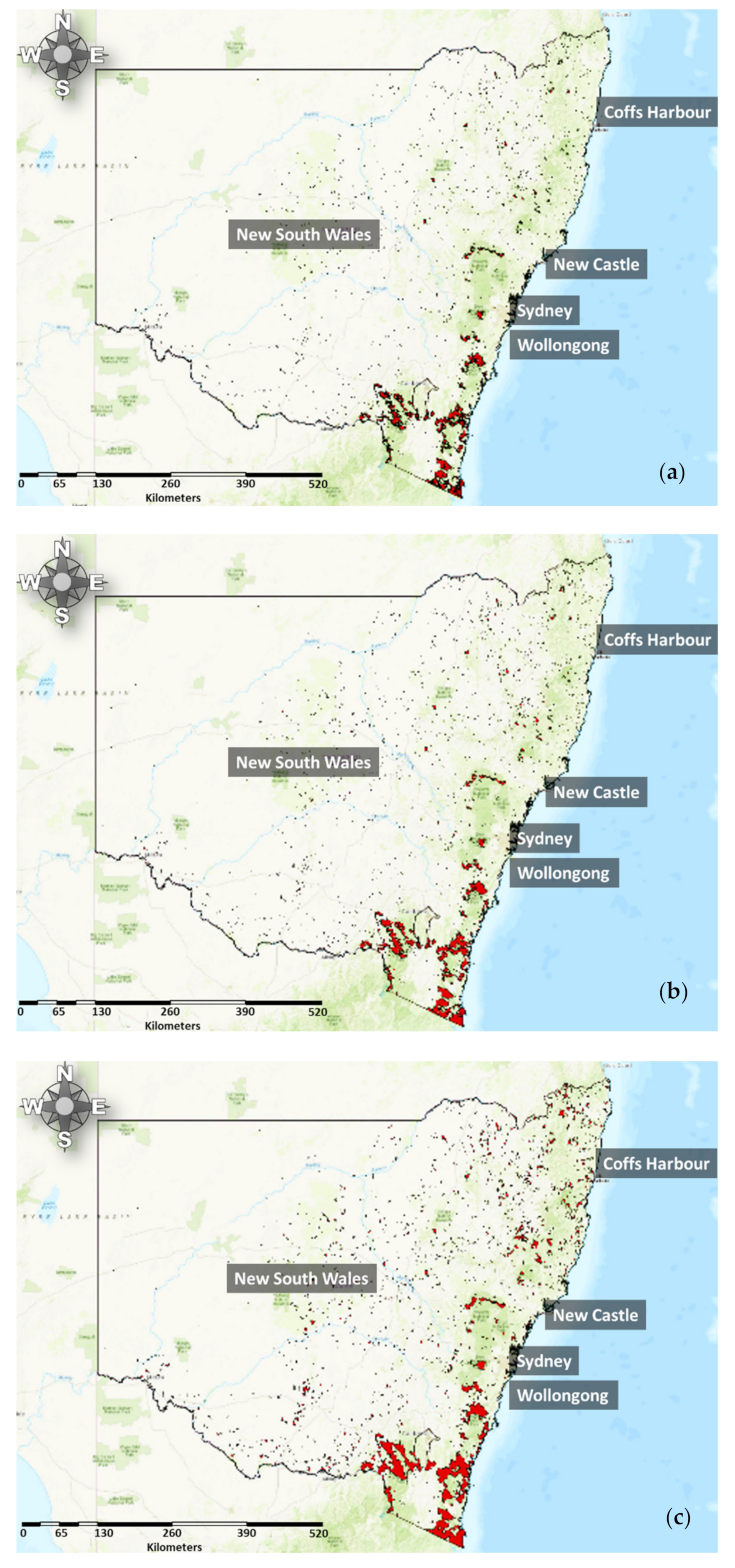
NOAA’s sensor, VIIRS fire product with 375 m resolution, is used to aggregate the perimeters of the fire with distances of 1 km, 2 km, and 5 km, as shown in Figure 7. The examples show the extent of the land damaged by the Black Summer fire season, where the burnt areas are shown in red colour. The maps show that the eastern part of the state is most affected by the fires. Significant, and more impactful, fire events have hit the cities along the coast, including Sydney, Coffs Harbour, New Castle, and Wollongong. The 1 km aggregates show that the sporadic distribution of the fires is largely spread throughout the state, as evident from Figure 7a. It depicts that each fire event has caused widespread damage. Likewise, the 2 km and 5 km aggregates show the land damages of the respective distances as shown in Figure 7b,c, respectively. The 5 km aggregates give the best depiction of the burnt area. The areas shown in this map include the southeastern region that connects NSW with the State of Victoria.

Additionally, the northern parts of the NSW are also heavily destroyed by these fires. Upon visual validation of the output with the Google Earth imagery, it is found that 50% of the national parks of NSW are impacted by the 2019–2020 fire season. This is in line with the NSW report that states a significant impact on NSW vegetation. These fires have resulted in damage of 2.5 million hectares of the state’s national parks [68].

4.2. Fire Clustering Patterns and the Significance

Figure 8 shows the level of clustering in the fire data, based on Get-Ord General G statistics generated through ArcGIS. The z-score is based on the randomization of the null hypothesis calculation. The distance method for the clustering analysis is Euclidean distance assessed based on inverse distance. The distance threshold for the state of NSW bushfire events is found to be 148,828.07 m. The higher z-score of 5.90 depicts a less than 1% likelihood that the events’ highly clustered pattern could be attributed to random chance. Therefore, these fire events are significantly high clustered along the entire state. Very strong clustering patterns can be visualized in Figure 8 towards the north and southeastern cities of NSW. Particularly in the southern parts, the clustering trend is quite pronounced mainly because the epicentre of the fire is near the Victoria NSW border region.

The statistical data generated by ArcGIS is presented in

Table 5. The statistical values of the data obtained from ArcGIS.

Assessment	Value
Observed General G	0.02
Expected General G	0.005
Variance	0.0
Z-Score	5.9
p-value	0.07

. As the z-score value is positive, and the observed General G index is larger than the expected General G index, high values for the attribute are clustered in the study area. Thus, more evenly distributed fires are experienced in NSW. Therefore, the null hypothesis is accepted as evident from the p-value of 0.07, which shows statistical significance when the p-value is greater than 0.05. Hence, it is confirmed that all the values linked with each feature are distributed randomly.

4.3. Monitoring of Bushfire Hotspots

The hotspot analysis, based on the Getis Ord Gi* statistics, is performed on the aggregated features of 5 km for ease of computation. Figure 9a shows the fire hotspots ranging in five categories: strong cold spots shown in dark blue, cold spots shown in light blue, nonsignificant spots shown in yellow, hotspots shown in orange, and strong hotspots shown in the red colour. Most of the NSW is covered sporadically with strong cold spots, primarily concentrated in the Pilliga Nature Reserve, Wollerni National Park, Yengo National Park, and the coastal regions in the north. Statistically, not-so-significant fire spots could be observed in Blue Mountain’s National Park and Morton National Park. Strong hotspots of bushfires are observed in the Deua National Park, situated in the southern part of the state. Some of the clear hotspots could also be observed in the Kosciu Sako National Park.

Similarly, Figure 9b illustrates the graph based on the z-score stats of the Get-Ord Gi* analysis. The graph gives an insight into the types of bushfire hotspots. The number of fires is plotted on the x-axis against their respective z-score values on the y-axis. The blue colour is densely populated across the study area and depicts that more than half of the state is included in the cold spots or strong cold spots. Some random parts of the state bushfires are shown in yellow, depicting that these events are not statistically significant. The relatively low z-score of 2.8–4.1 can be seen in the orange colour, which shows a good clustering of hotspots. On the contrary, the strong z-score values above 4–10.5 depict strong clusters of severe hotspots in the study area. Though these strong hotspots are not so thickly populated across the study area, they impacted the fires throughout the state.

Figure 10 shows the complete picture of the bushfire hotspots in the state of NSW. The graduated size of circles shows the intensity of the hotspots across the study area. The map shows that the fire events have severely hit the eastern regions of NSW. Minor hotspots of bushfires are densely and randomly dispersed throughout the study area. The noteworthy and more impactful hotspots are shown in a bigger circle in southeastern NSW. These include the Deua National Park, Morton National Park, and Kosciu Sako National Park. Other larger hotspots are in the northeast in the Wollerni and Yengo National Parks. These regions were already at risk of fires, considering the weather conditions of hot maximum temperatures, dry and humid incidents, and the prevalent fire weather situations. Further, it points out that the upcoming fire events will be more frequent and severe than ever recorded before [6]. Thus, the government must act and put measures in place before the next fire event.

4.4. Regression Analysis of the Black Summer Fires

Most of the northern and central areas of the NSW have observed extremely low precipitation in the year 2019. Some of these locations recorded the driest conditions in history. Lower rainfalls impacted the water resources and the associated firefighting mitigating measures [69]. By the start of August, almost the entire NSW was stricken by severe drought (55%), observing drought conditions (23%), and experiencing extreme droughts (17%). The initial ‘Section 4.4 emergency’ was declared on 10 August 2019 [70]. 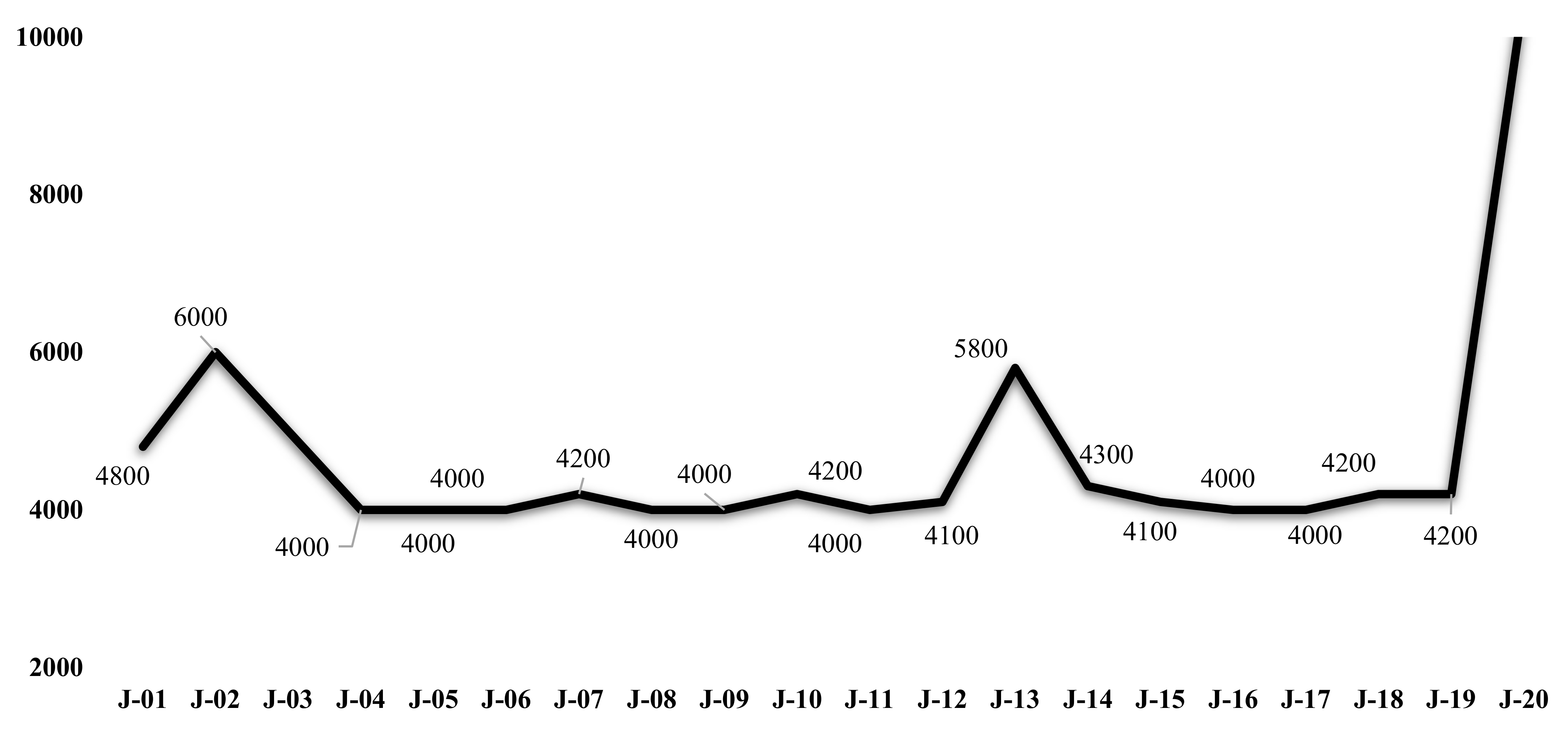Additionally, adequate soil moisture deficits and prevalent winds facilitated the considerable frequency of fire events [71]. A total area of 5,595,739 hectares was burnt, destroying 2475 houses, and causing 25 casualties by 10,520 fire incidents in NSW, as shown in Figure 11.

These fires of NSW made a record of burning more area than any other fire season in the past two decades, as seen in Figure 11, that the authors compiled based on the data available online. Figure 11 shows data for January of each odd calendar year starting from 2001 till 2019, where the number of fires is plotted. The 2019 fires have been the worst disaster in terms of the number of fires and areas burnt. The year 2012 had the least burnt area and lower numbers of fire, followed by 2008 and 2004.

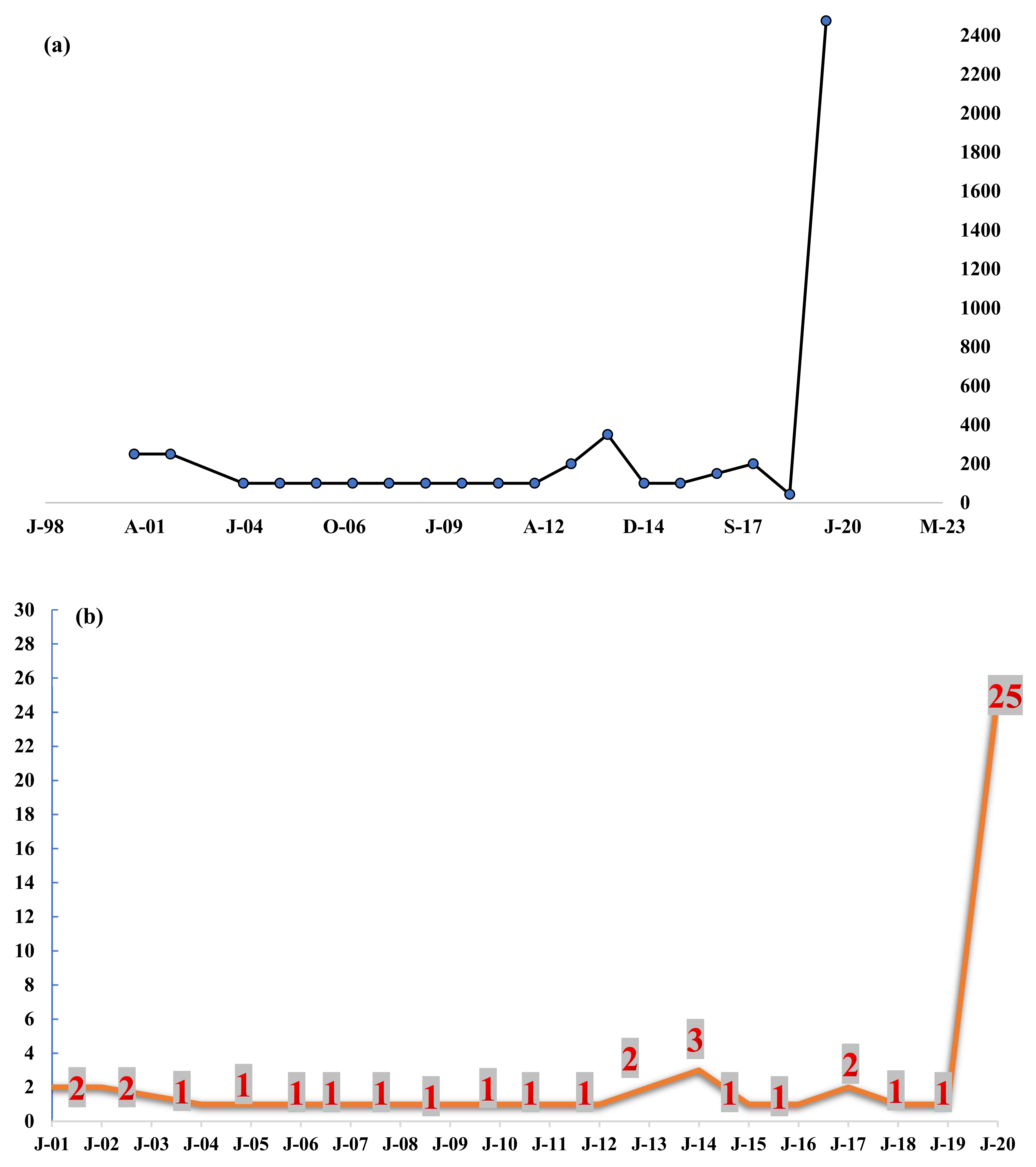
Figure 12 shows the data for houses burnt and the fatalities of various fires in NSW since 2001. All the data is plotted for the reports of January of the particular year. The authors compiled the data based on online information and reports of the parliament of Australia and NSW RFS. The Black Summer fire season has been an extraordinary disaster where the burnt area, fatalities, and damaged houses are more significant than the previous years. Before the 2019 season, the notable instances are 2001 and 2002 fires, with 250 houses damaged and two fatalities each. The 2013–2014 fires resulted in the loss of three lives and damages to 350 houses. Similarly, 2013 and 2017 also resulted in the loss of two lives and damages to approx. 200 properties.

In

Table 6. Regression Analysis for 2001–2020 fire seasons in New South Wales.

Impact Factors	Standard Error	p	r	R2
Fire Season (y) vs. Burnt Area (x)	1,288,108	0.019	0.59	0.35
Fire Season (y) vs. Houses Loss (x)	52,737	0.12	0.39	0.15
Fire Season(y) vs. Life Loss (x)	5.30	0.11	0.40	0.16
Burnt Area(y) vs. Fire Season (x)	1639	2.75 × 10–19	0.59	0.31
Life Loss (y) vs. Houses Loss (x)	0.36	0.54	0.99	0.99

, before the Black Summer fires, the trend of the burnt area showed a negative slope, transitioning into a positive with the 2019–2020 fires, signifying a p-value of 0.019. The frequency of fires has been decreasing until 2012 that started to increase post-2012. It showed a positive trend for the dataset with a greater slope for 2001–2020. The data analysis shows a positive linear relationship between the fire events and the burnt area that is found to be statistically significant with a p-value of 0.59. A regression line for the house damaged over the years shows a positive slope. It shows a statistically significant p-value of 0.12. Due to the 2019–2020 fire season data, a statistically significant output with a p-value of 0.54 is obtained. Fatalities are estimated to be about 1% of the houses damaged. This dataset shows an error of 0.36 for the fatalities. The results are similar to an extensive study performed by Filkov et al. [72], where the researchers explored the impact of the recent fires on the houses and lives lost.

4.5. UAV Routing Results

As discussed in the Method Section, the UAVs’ paths were optimized using the PSO algorithm to have the shortest possible distance for monitoring the fire events. For doing this, different cases are considered in the target area of NSW Australia. Varying iterations, number of UAVs, computation time taken by the control unit, and the best (shortest) travel distance for UAVs are presented in

Table 7. Test cases with the number of iterations, UAVs, elapsed computation time, and optimized distance.

No. of Iteration (I)	Number of UAVs (n)	Elapsed Time(s)	Best Transportation Distance (km)
50	20	14.64	12.89
	40	16.24	12.97
	60	18.49	13.24
	80	20.34	13.18
	100	22.07	12.81
100	20	28.36	13.08
	40	32.65	12.85
	60	35.65	12.92
	80	40.03	13.16
	100	43.20	12.80
200	20	57.37	12.82
	40	63.72	12.80
	60	71.12	12.86
	80	78.85	12.91
	100	85.14	12.80
300	20	85.37	13.24
	40	96.17	13.33
	60	106.80	13.34
	80	116.07	13.21
	100	128.06	12.82
400	20	110.97	13.09
	40	123.71	13.01
	60	139.32	12.86
	80	152.12	13.19
	100	167.84	12.80
500	20	137.37	13.20
	40	153.32	13.21
	60	173.50	13.01
	80	191.89	12.85
	100	204.85	12.82

. The iterations include 50, 100, 200, 300, 400, and 500, whereas the number of UAVs is varied between 20, 40, 60, 80, and 100 for each iteration. From Table 7, in most of the cases, 20 UAVs give the best results for computation speeds, and 100 UAVs give the best transportation distance to be covered (shortest distance). The computation time ranges from 14.64 s for 20 UAVs and 50 iterations to 137.37 s for the same number of UAVs with 500 iterations. On average, the optimized distance is around 12.81 km of area, which is a considerable distance, considering the limited battery operating time of the UAV. This shows that the more UAVs there are in the swarm, the better the results will be, as the UAVs can communicate with more UAVs in the swarm and share the workload more efficiently. Thus, depending on the area to be covered, the UAVs in the swarm should be increased. The values are generated through the MATLAB code for PSO to optimize the UAV routes.

There is a trade-off between computational time and transportation cost. Moreover, considering the number of iterations to be 200 and 400 for 100 UAVs, the best transportation distance is the same (12.80 km); however, the elapsed time is 85.14 and 167.84 s. This shows that the time can vary even with the same cost; hence, there is no universal rule for selecting a definite number of UAVs or inferring that the maximum number of UAVs will give minimum cost in all cases.

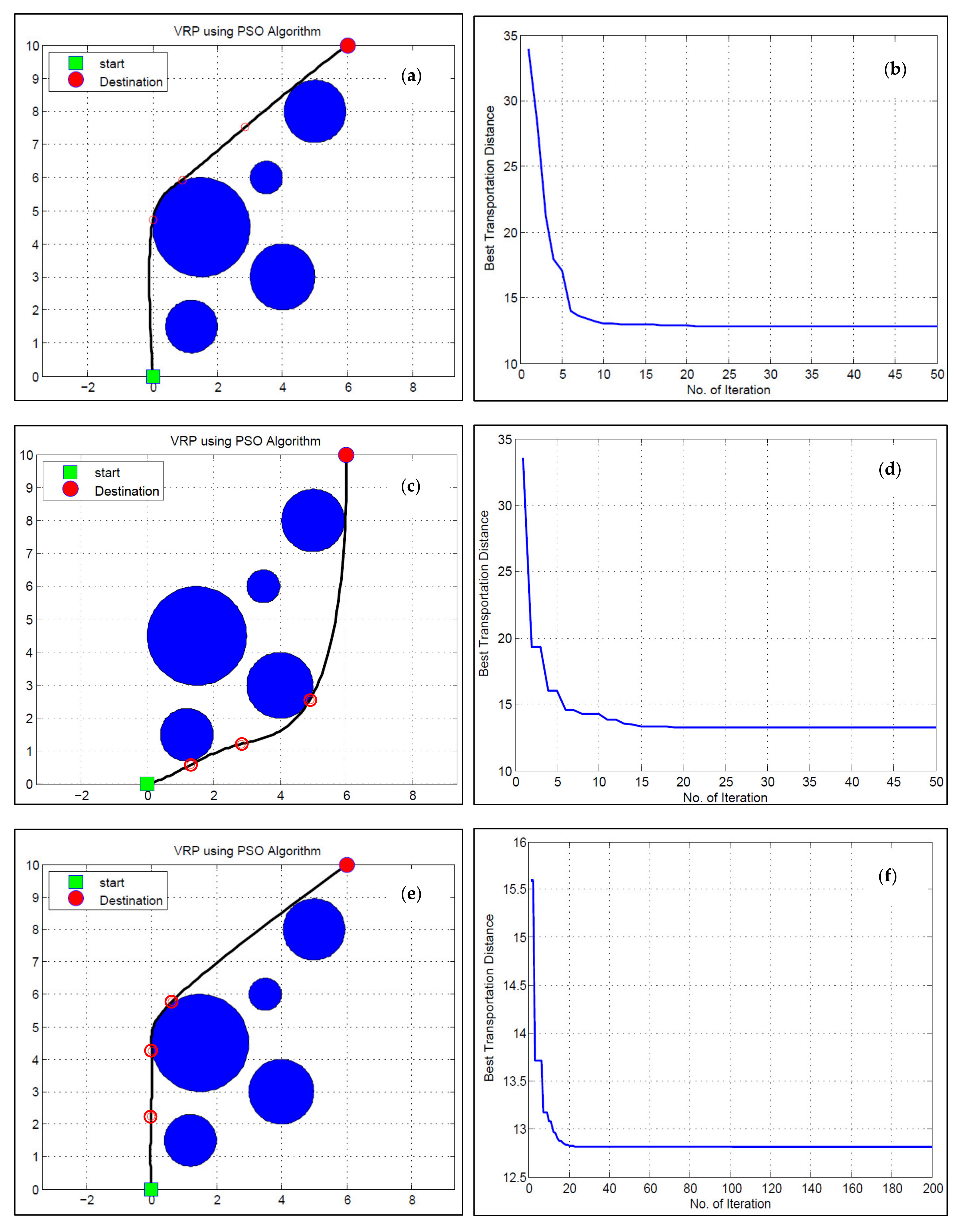
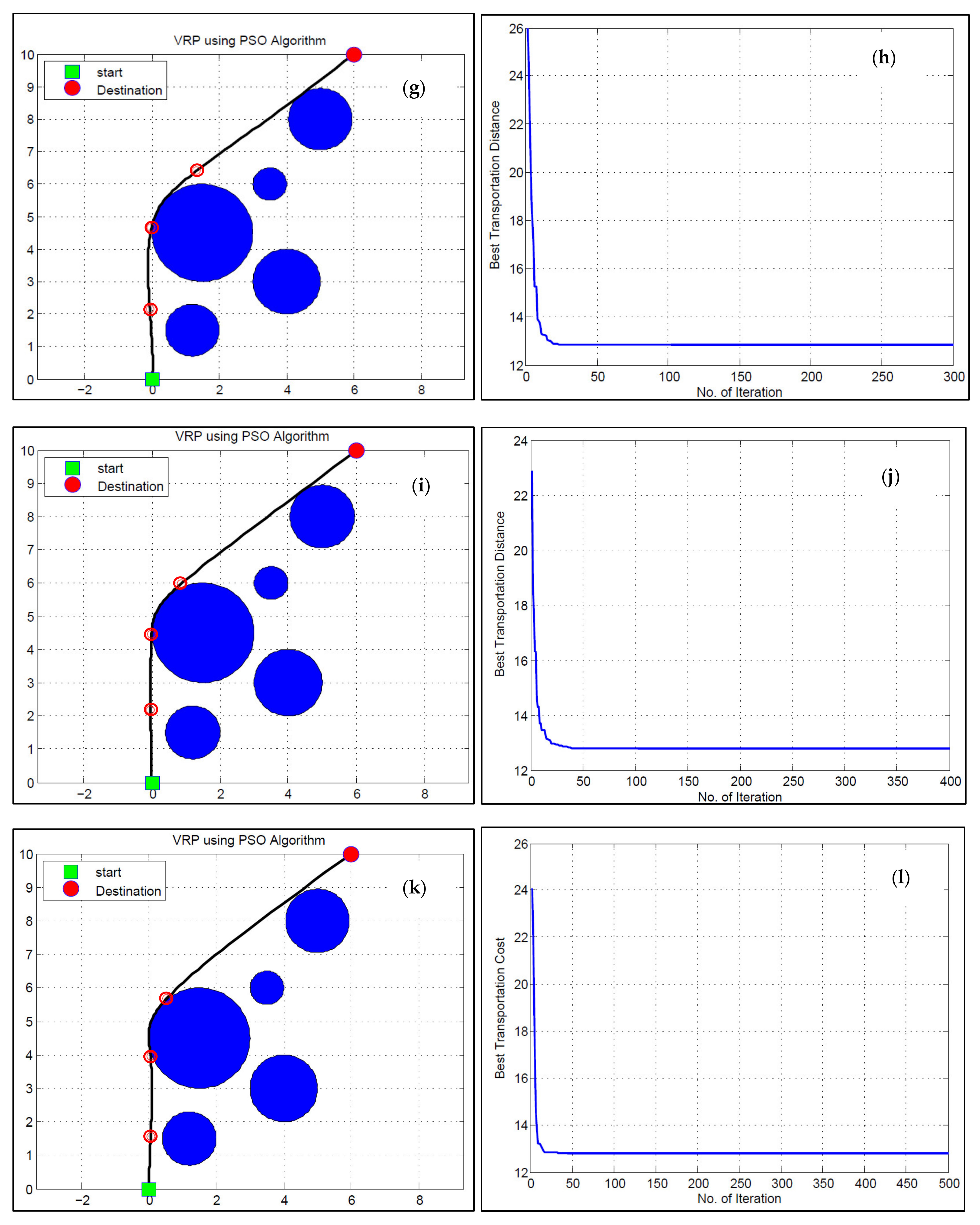
Figure 13 shows the iteration results for all test cases involving 100 UAVs. The optimal UAV path for detecting bushfires is simulated in the MATLAB environment. For this purpose, a PSO algorithm is designed based on certain parameters such as iteration, population size, inertial weight, damping ratio, as well as personal and global learning coefficient to calculate the best transportation distance. Figure 13a,c,e,g,i,k illustrates a 2D scenario of UAV routing problem from starting point to destination. Blue circles are the obstacles in the UAV trajectory. The best transportation distance and elapsed time are calculated based on the UAV hovering from the start to the destination, where the effect zone (bushfire) needs to be monitored. Three handle points, indicated in light red circles, are considered to smoothen the path from start to destination. The x and y-axis represent the lengths and widths of the plots or locations (P1 to P10). Figure 13b,d,f,h,j,l shows the best transportation distance, concerning number of iterations. In all the cases, the case study area’s optimized distance with 100 UAVs is 12.81 km, on average. When the iterations are increased from a specific point, the distance follows a straight path. In the case of the lower number of UAVs, the optimized distance is increased, which means lower productivity and more battery losses. Thus, it is advised to use more UAVs in the swarm for better results and less travel distances for swift disaster response.

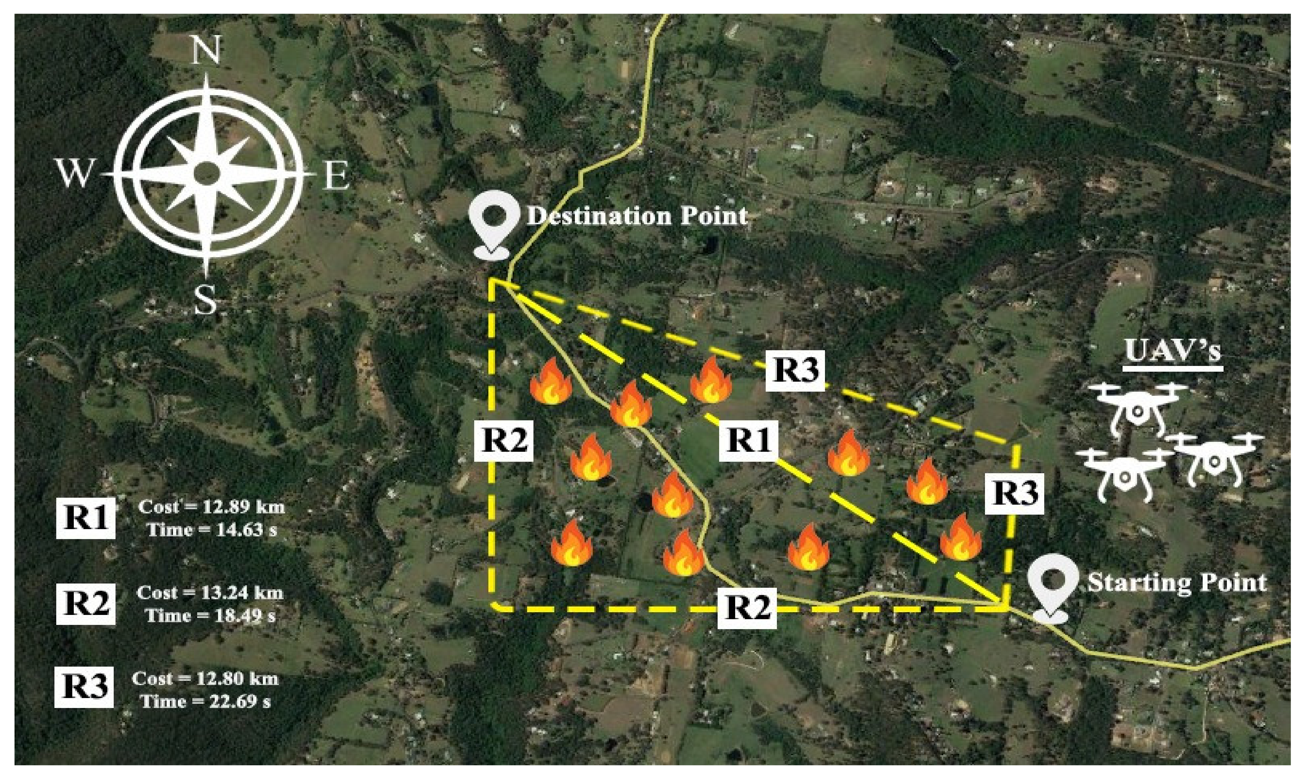
Figure 14 shows a swarm of UAVs deployed at a test zone at NSW with their starting points, destination point, and various possible routes. Using PSO, the Route 1 value is 12.89 km with a computation time of 14.63 s. Route 2 takes 18.49 s and gives an optimized path of 13.24 km, whereas Route 3 has values of 12.80 km for the optimized path and takes 22.69 s to be computed. Depending upon the scenario, if computation time is not the highest priority, R3 has the best results for the optimized path. However, if computation speed is the concern, Route 1 has the best values with just 14.63 s of computation time. Thus, the trade-off between computation speeds and optimized routes may be input into the control units through artificial intelligence or human presence. This decision can be taken in real-time at the control unit or head office through remote administration.

Accordingly, the NSW and the rest of Australia can be covered through UAV swarms whose paths are optimized through PSO algorithms to tackle any bushfire disaster. The proposed system can be adopted by the NSW RFS to plan for upcoming fire seasons actively. The system, if adopted, can help save lives, reduce the bushfire impacts on properties and livestock, and save many species of wildlife from bushfire disasters. With the growing availability of UAVs, the proposed system will cost way less than the post-disaster rehabilitation and repairs. Vigilant and swift policy making is required in this context to help mitigate the harmful effects of bushfires disasters by adopting the proposed system.

The area covered depends on the availability of UAVs and the technology level used in the UAVs. As far as the costs associated with the increased number of UAVs are considered, it can be estimated using the area coverage path planning, which depends on finding the route that covers every point within the target area of interest [73]. Particularly, for our system, the costs of using an increased number of UAVs will be greatly dependent on the area coverage path planning for our area of interest.

In various disastrous situations, many UAVs can be effectively deployed, as the utility of UAVs is highly implicated and appreciated in such future situations. The UAVs can play promising roles in various relief efforts in natural disaster situations such as bushfires, storms, and earthquakes. Notably, UAVs can perform very crucial jobs as soon as disasters emerge. These tasks include identifying people in emergencies who require urgent help. Greater evidence supports the fact that UAVs display several advantages over traditional searching and rescuing with a considerably higher speed. UAVs can perform additional roles, such as delivering the rescue ropes and life jackets in dangerous areas where ground-based rescue efforts are practically impossible and very difficult. These UAVs have an inherent ability to assess the damage caused to infrastructures such as roads, buildings, tunnels, bridges, etc. Different types of models can be effectively coupled with these systems. Some of the most prominent examples are the traditional continuum model, expand contract model, and disaster crunch model. The traditional continuum model is based on sequential stages, focusing on the activities associated with pre-disaster and post-disaster events. Our proposed systems can be effectively used if integrated with such types of models. The coupling of our systems to these models will speed up and enhance the projection, which will help attain an improved response from the governing bodies. If the governing bodies for disaster management extend their support, UAVs can be effectively used in natural disasters such as floods, bushfires, etc.

During the post-disaster assessment, the battery life of the UAV plays a significant role in hovering time. In a recent study by Fotouhi et al. [74], the authors implemented a control strategy for confined Phantom 4 mobility using a DJI software development kit (SDK). Considerably, the speed of the UAV is directly proportional to the power utilized. The pertinent results shows that the power utilization abruptly reaches 167 W, as the UAV speed peaks to 10 m/s.

UAV battery consumption is always an important issue to address, keeping the sustainability of technology in mind. A solution for the UAV battery energy consumption is proposed in Selim and Kamal [75] using UAV Base Station (UAV-BS) and Powering Drone (PD). The PD provides the necessary charging for the hovering UAV-BS to make it more efficient for monitoring the affected area without going back to the depot and providing the optimum results. In the relevant study, during the initial timing block, from 0 to 1, the UAV-BS are initialized from 200 kJ capacity and consume the maximum energy to reach the allocated spot.

5. Conclusions

The current study investigated the devastating 2019–2020 Black Summer fires occurring in NSW Australia. Using the case study of the NSW region of Australia, GIS and remote sensing analyses were conducted to map the burnt areas of NSW. The results highlight that 50% of the national parks of NSW were impacted by the 2019–2020 fire season, resulting in damage to 2.5 million hectares of the state’s national parks. The fire clustering patterns indicated that these events are significantly, highly clustered in the entire state, where very strong clustering patterns can be visualized towards the north and southeastern cities of NSW. The clustering trend is quite pronounced on the southern side of NSW, where it shares the border with Victoria.

Similarly, the hotspot mapping shows that strong hotpots of bushfires are in the Deua National Park, situated in the southern part of the state, and the Kosciu Sako National Park. Other larger hotspots are in the northeast in the Wollerni and Yengo National Parks, which had been declared to be at risk by the government due to weather conditions of hot maximum temperatures, dry and humid incidents, and the prevalent fire weather situations. The government must act and enact measures before the next fire event; otherwise, the data trends show that upcoming fires could be more devastating than the Black Summer.

A UAV-based bushfire monitoring system is proposed in the current study to monitor the bushfires in NSW and instigate a swift response plan to minimize the losses. The paths of the UAVs are planned and optimized using the PSO algorithm for avoiding barriers in the path and covering the maximum area in the shortest possible time. The test results with 50, 100, 200, 300, 400, and 500 iterations and the number of UAVs varying between 20, 40, 60, 80, and 100 for each iteration show that 20 UAVs give the best results for computation speeds, and 100 UAVs give the best transportation distance to be covered. Thus, the more UAVs are there in the swarm, the better will be the results in most cases. These UAVs can communicate with more UAVs in the swarm and share the workload more efficiently if the number is higher. Thus, it is proposed to increase UAVs if more area is to be covered and monitored.

The current study is limited to test cases without submission to field tests due to the non-fire seasons. In the future, it can be tested in the field, and real-time results can be assessed to test the in-field validity and performance of the proposed method. Nevertheless, it is a first step towards addressing a key issue of bushfire disasters in the Australian context that other countries in the world can adopt. For Australia and NSW, the RFS can adopt the proposed system and have the UAV swarm ready before the next fire season to instantly map, assess, and mitigate bushfire disasters. Further, it is recommended to develop a shared, integrated platform for diverse data sources, intelligence, and information sharing across government organizations where useful data can be shared. New wildfire risk assessments should be conducted with high-resolution mapping technologies to assess the current state of wildlife and help place protection measures in place. The scientific understanding of “megafires” should be enhanced through retrospective analysis and fire behaviour models, and associated inputs for real-time prediction should be investigated. These, when achieved in their true essence, will help lay the foundation of enhanced environmental sustainability for industry 5.0.