A Study into the Availability, Costs and GHG Reduction in Drop-In Biofuels for Shipping under Different Regimes between 2020 and 2050

Abstract

In this study, various scenarios were developed that correspond to estimations of future biomass availability and biofuel demand from the maritime industry. These marine biofuel demand scenarios were based on the Greenhouse Gas (GHG) reduction targets of the Renewable Energy Directive II (RED II) and the International Maritime Organization (IMO). A multi-objective Mixed Integer Linear Programming (MILP) model was developed which is used to optimize the Well-to-Tank (WtT) phases of each studied scenario. This resulted in an overview of the most feasible use of feedstocks, deployment of new conversion technologies and trade flows between regions. Additionally, the results provided insight into the costs and emission reduction potential of marine biofuels. By analyzing the results from this study, improved insight into the potential of drop-in biofuels for reaching the proposed emission reduction targets for the maritime sector was developed. A trade-off between costs and emissions was found to result in potential GHG reductions between 68–95% compared to Heavy Fuel Oil (HFO) for 800–2300 EUR/ton. More specifically, 80% GHG reduction compared to HFO can be achieved at fuel costs of between 900–1050 EUR/ton over the studied time period.

1. Introduction

The shipping sector is responsible for about 90% of international freight transport [1]. Emitting 2.8% of worldwide Greenhouse Gas (GHG) emissions, the share in air pollution of the shipping sector is about the size of Germany [1,2]. Although the relative emissions per unit of cargo are low compared to other transport modes, the total share in emissions of the shipping industry is significant [3,4,5]. At this stage, the major part of the world shipping fleet still runs on fossil fuels. In addition, the harmful emissions caused by the combustion of fossil fuels, other factors such as the finite oil supply and the sustainability of the oil supply chain create the need for alternative propulsion solutions [6].

In order to decrease air pollution caused by the maritime industry, the International Maritime Organization (IMO) implemented regulations that limit nitrogen oxide emissions and the use of high sulfur fuels. However, regulations that limit GHG emissions from shipping are at this stage non-existent. The European Union (EU) implemented the Renewable Energy Directive II (RED II), which contains an obligation for the share of renewable fuels in the transport sector, but shipping is excluded. Nevertheless, the IMO has set the ambitious goal to decrease absolute GHG emissions from shipping by 50% by 2050 compared to 2008 levels.

To reach this target, Bouman et al. [7] evaluated several potential emission reduction measures for shipping. This analysis showed that biofuels have a considerable potential to reduce GHG emissions emitted by ships. Biofuels are one of the few renewable fuels that are commercially available at this stage. The first generation of biofuels was primarily based on plant oil but this could result in indirect land use and deforestation. This is a concern when striving for sustainable shipping [8]. The second generation of biofuels does not have this issue, and the optional sources are outlined also in the mentioned RED II of the EU. Additionally, biofuels contain negligible amounts of sulfur and are in line with current regulations. A distinction can be made between drop-in biofuels and non drop-in biofuels. Drop-in biofuels can be blended gradually into the existing fuel mix. The usage of drop-in biofuels ensures that little to no adjustments are required relative to existing fuel infrastructure. Non drop-in biofuels include alcohols such as (m)ethanol and gaseous fuels which cannot be used in a diesel engine without adjustments. In this study, the potential of drop-in biofuels is addressed. Based on their suitability as a marine fuel and their drop-in character, five drop-in biofuels are selected for this study. These fuels include Fatty Acid Methyl Esters (FAME), Hydrotreated Vegetable Oil (HVO), Fast-Pyrolysis with full hydrodeoxygenation (FP), Hydrothermal Liquefaction with full hydrodeoxygenation (HTL) and Gasification with consequent Fischer–Tropsch synthesis (GFT). Biomass types used as feedstock for these fuels were categorized using the categorization shown in

Table 1. Feedstock categorization used in this thesis. Partly adapted from De Jong et al. [9].

Feedstock Category	Feedstocks
Vegetable oils	Palm, sunflower, soybean and rapeseed
Waste oils	UCO and tallow
Agricultural residues	Grain residues
Forestry residues	Primary: Leftover from logging operations, early thinning or final felling (branches, stumps, tree tops, bark and sawdust, etc.) Secondary: by-products and co-products of industrial wood-processing operation (bark, sawmill slabs, sawdust and wood chips, etc.)
Energy crops	Miscanthus, willow and poplar
Solid waste	Municipal solid waste
Liquid waste	Animal manure and wastewater sludge

.

Drop-in biofuels have the potential to decrease GHG due to the principle of a short-carbon cycle. In contrast to fossil products, the biomass used as a feedstock for biofuel production absorbs CO${}_2$ from the air during their lifetime. When the biofuel is combusted, the same amount of CO${}_2$ is released into the air. When considering waste products for this, there is no competition for land use in that manner. The net emission are, therefore, considered zero. However, biomass is not evenly spread across the globe, which might cause regions to import or export large quantities of feedstock [10,11]. Therefore, the production and transport emissions cannot be disregarded and should be considered as emissions for the fuel. Hence, production and transport largely determine the sustainability of the biofuel. This induces the need for both transport and production of biofuels. Therefore, to reduce costs and emissions, both production and transport need to be optimized. This study aims to provide an improved insight into the potential of drop-in biofuels for reaching the proposed emission reduction targets for the maritime sector. By approaching the transportation of biofuels as a multi-objective optimization, a variation in focus between economics and GHG emissions can be studied in order to identify the potential in reduction against an acceptable cost.

2. Materials and Methods

In order to fill the indicated knowledge gap, the following methodology is used:

• Model the marine biofuel supply chain;
• Determine the availability of feedstocks;
• Determine the future demand for marine biofuel;
• Determine the required model parameters;
• Perform a scenario analysis.

Starting with the development of a multi-objective strategical supply chain optimization model, these steps are executed chronologically.

2.1. Mathematical Model Formulation

This section contains the mathematical formulation of the multi-objective Mixed Integer Linear Programming (MILP) model. The corresponding nomenclature is provided. A schematic representation of the model is given in Figure 1. The world is divided into 18 regions in which the main bunker hubs are used as nodes in the network. The following subsections contain the economic objective, environmental objective and model constraints.

2.1.1. Economic Objective

The economic objective is to minimize total system costs. These total system costs are dependent on four decision variables. Three of these decision variables are related to the flow inside the system and are continuous. The fourth is an integer variable which indicates how many refineries of size $p\in P$ and type $g\in G$ are located at refinery node $r\in R$. The decision variable $B{F}_{sbjit}$ indicates the amount of biomass of type $b\in B$ of supply interval $i\in I$ that is processed into intermediate $j\in J$ at supply node $s\in S$ during time period $t\in T$. The decision variable $I{F}_{srjt}$ specifies the flow of intermediate product $j\in J$ that is transported from supply node $s\in S$ to refinery node $r\in R$ during time period $t\in T$. The decision variable $F{F}_{rdgt}$ reveals the amount of biofuel type $g\in G$ that flows between refinery node $r\in R$ and demand node $d\in D$ during time period $t\in T$. The final decision variable, $Y_{rgpt}$, indicates if a refinery of size $p\in P$ producing fuel $g\in G$ is operational at the candidate location $r\in R$ during time period $t\in T$.

These four decision variables, combined with several parameters, are used to formulate the following economic objective function.

$$Ob{j}^{eco}=Min.C$$

(1)

Total costs can be separated into three parts: the costs of the intermediate product, the costs of upgrading the intermediate to a biofuel and the cost of sea transport.

$$C=\sum _{t\in T}(C_t^I+C_t^U+C_t^T)$$

(2)

Costs of the intermediate product are dependent on the region and the feedstocks that they are made from. It is assumed that a processing facility in a certain area only uses feedstocks that originate from that area. These costs can again be subdivided into three parts. The costs related to the intermediate product consist of feedstock, processing and inland transport costs.

$$C_t^I=C_t^{IB}+C_t^{IP}+C_t^{IT}$$

(3)

The feedstock costs are the costs of the different types of biomass $b\in B$ at location $s\in S$ during time period $t\in T$.

$$C_t^{IB}=\sum _{s\in S}\sum _{b\in B}\sum _{j\in J}ub{c}_{sb}·B{F}_{sbjit}\forall t\in T$$

(4)

The processing costs are expressed as the costs related to producing intermediate product $j\in J$ from biomass type $b\in B$ at supply location $s\in S$. An assumption is made that the processing costs are only dependent on the area in which the processing is performed. Spatial optimization of the processing facilities is outside the scope of this thesis. The reason for this is the assumption that long-distance transport of low-density biomass would not be efficient. Therefore, smaller distributed processing facilities would always be located near the harvest site.

$$C^{IP}=\sum _{s\in S}\sum _{b\in B}\sum _{j\in J}up{c}_{sj}·I{F}_{srjt}\forall t\in T$$

(5)

The third part of $C_t^I$ includes the inland transport of the biomass to the processing facility. Generally, the supply costs of biomass are depicted as cost/supply curves. Regional biomass costs rise when the required supply increases. Initially, biomass that is nearest to the processing facility and most easy to gather is used. When demand increases, biomass that is more difficult to access and is further from the processing facility will be used, increasing transport distance and costs consequently. In order to mimic this, inland transport costs are expressed as a linear function of the biomass flow inside the supply areas. However, this property induces a non-linear relationship between the biomass flow and inland transport costs. Therefore, the function is cut up into five discrete cost segments for every biomass type and region combination.

Using the above described method, the total inland transport costs of biomass for every $t\in T$ can be calculated using the following expression. Observing that biomass is usually of low density, the volume is assumed to be the limiting factor.

$$C_t^{IT}=\sum _{s\in S}\sum _{b\in B}\sum _{j\in J}(uit{c}_s·{\rho }_b·\frac{B{F}_{sbjit}}{lhv{b}_b})\forall t\in T$$

(6)

The second cost item includes the costs that are related to setting up and operating an upgrading facility. These costs can be divided into variable and fixed costs.

$$C_t^U=C_t^{UV}+C_t^{UF}\forall t\in T$$

(7)

In the optimization model of Lin et al. [12], the Operational Expenses (OPEXs) were considered to be independent of the refinery capacity. In this model, the same assumption is made. However, OPEXs are dependent on the location in which the refinery operates. The OPEXs are calculated separately from the feedstock costs, which were already included in $C_t^{IB}$.

In general, part of the OPEX can be seen as variable costs and another part as fixed costs. $C^{UV}$ only includes the variable part of the OPEX, which is dependent on the produced amount of biofuel.

$$C_t^{UV}=\sum _{r\in R}\sum _{g\in G}\sum _{d\in D}uv{c}_{rgt}·F{F}_{rdgt}\forall t\in T$$

(8)

In Equation (8), $uv{c}_{rgt}$ represents the OPEX per energy output of biofuel $g\in G$ at location $r\in R$ during time period $t\in T$. The Capital Expenses (CAPEXs) are annualized over the lifetime and are added to the fixed part of the refinery OPEX. This is expressed in Equation (9).

$$C_t^{UF}=\sum _{r\in R}\sum _{g\in G}\sum _{p\in P}uf{c}_{rgpt}·Y_{rgpt}\forall t\in T$$

(9)

The decision variable $Y_{rgpt}$ is an integer that indicates if a plant of size $p\in P$ producing fuel $g\in G$ at location $r\in R$ is operational during time period $t\in T$.

Lastly, transport costs are divided into the costs for the transportation of the intermediate products and the end products.

$$C_t^T=C_t^{IT}+C_t^{FT}\forall t\in T$$

(10)

$$C_t^{IT}=\sum _{s\in S}\sum _{r\in R}\sum _{j\in J}(ust{c}_{sr}·\frac{I{F}_{srjt}}{lhv{j}_j})\forall t\in T$$

(11)

$$C_t^{FT}=\sum _{r\in R}\sum _{d\in D}\sum _{g\in G}(ust{c}_{rd}·\frac{F{F}_{rdgt}}{lhv{g}_g})\forall t\in T$$

(12)

2.1.2. Environmental Objective

The environmental objective is to minimize the total GHG emissions related to the supply of marine biofuels. The same decision variables as introduced in the previous section are used for the environmental optimization. In order to determine the GHG emissions of the marine biofuel supply chain, the method of Giarola et al. [13] is used as a starting point. The life-cycle emissions are separated into different phases. The objective is to minimize total system emissions, as expressed in Equation (13).

$$Ob{j}^{env}=Min.E$$

(13)

These total system emissions can be divided into emissions related to the intermediate bio-energy carrier, upgrading the intermediate to a biofuel and transport, which can be evaluated as follows.

$$E=\sum _{t\in T}(E_t^I+E_t^U+E_t^T)$$

(14)

Firstly, an expression that represents the emissions caused by the production of the intermediate bio-energy carrier is developed. These emissions can be split up into emissions caused by harvesting, gathering and processing of the feedstocks. Moreover, inland transport of the feedstock needs to be considered.

$$E_t^I=E_t^{IB}+E_t^{IP}+E_t^{IT}\forall t\in T$$

(15)

Emissions caused by harvesting and gathering of the feedstocks are assumed to be proportional to the flow of biomass inside the supply regions.

$$E_t^{IB}=\sum _{s\in S}\sum _{b\in B}\sum _{j\in J}B{F}_{sbjt}·e{f}_{sb}\forall t\in T$$

(16)

Furthermore, the feedstock will be processed into an intermediate energy carrier. The emissions related to this conversion are proportional to the amount of intermediate produced.

$$E_t^{IP}=\sum _{s\in S}\sum _{r\in R}\sum _{j\in J}I{F}_{srjt}·e{p}_{sj}\forall t\in T$$

(17)

The inland transport costs are considered as a constant for every region and biomass type. An average distance is assumed dependent on the size of the region. Furthermore, the same approach as explained in Section 2.1.1 is used to simulate increasing inland transport emissions due to increasing distance when more supply is needed.

$$E_t^{IT}=\sum _{s\in S}\sum _{b\in B}\sum _{j\in J}B{F}_{sbjt}·\frac{ei{t}_{sb}}{lhv{b}_b}\forall t\in T$$

(18)

For the emissions related to the upgrading of the intermediate bio-energy carrier to the eventual biofuel, the following expression is used.

$$E_t^U=\sum _{r\in R}\sum _{d\in D}\sum _{g\in G}F{F}_{rdgt}·e{u}_g\forall t\in T$$

(19)

Additionally, there are emissions associated with the overseas transport of both the intermediate bio-energy carrier and the biofuel.

$$E_t^T=E_t^{TI}+E_t^{TF}$$

(20)

These emissions are caused by the combustion of fossil products of the tankers which transport the goods. Both the flow of the intermediate products and the biofuel products are multiplied with an emission factor that is dependent on the distance between the nodes.

$$E_t^{TI}=\sum _{s\in S}\sum _{r\in R}\sum _{j\in J}I{F}_{srjt}·es{t}_{sr}\forall t\in T$$

(21)

$$E_t^{TF}=\sum _{r\in R}\sum _{d\in D}\sum _{g\in G}F{F}_{rdgt}·es{t}_{rd}\forall t\in T$$

(22)

2.1.3. Constraints

Firstly, all four decision variables are not allowed to take on negative values.

$$B{F}_{sbjit}\ge 0\forall s\in S,b\in B,j\in J,i\in I,t\in T$$

(23)

$$I{F}_{srjt}\ge 0\forall s\in S,r\in R,j\in J,t\in T$$

(24)

$$F{F}_{rdgt}\ge 0\forall r\in r,d\in D,g\in G,t\in T$$

(25)

$$Y_{rgpt}\ge 0\forall r\in R,g\in G,p\in P,t\in T$$

(26)

Secondly, flow equilibrium constraints are required to ensure that the flow of goods stays consistent throughout the solution. Equation (27) ensures equilibrium in every supply node between biomass flow in and intermediate flow out.

$$\sum _{b\in B}(B{F}_{sbjit}·{\omega }_{bj})-\sum _{r\in R}I{F}_{srjt}=0\forall s\in S,t\in T,j\in J$$

(27)

Equation (28) is established to ensure equilibrium in all refinery nodes.

$$\sum _{s\in S}\sum _{j\in J}(I{F}_{srjt}·{\gamma }_{jg})-\sum _{d\in D}F{F}_{rdgt}=0\forall r\in R,g\in G,t\in T$$

(28)

An additional constraint is used to prevent flow from going through nodes where no refinery is built. For this purpose, the big-M method is used. M represents a new parameter to which a large number is assigned. Hence, a yes or no decision can be formulated as follows.

$$\sum _{p\in P}{Y}_{rgpt}·M\ge \sum _{d\in D}F{F}_{rdgt}\forall g\in G,r\in R,t\in T$$

(29)

In order to ensure that the global biomass availability is not exceeded, a constraint is required per region that limits the amount of biomass used by all ports in that region. For every distinct region in H a separate constraint is composed, shown in Equation (30).

$$\sum _{j\in J}B{F}_{sbjt}\le fca{p}_{hbt}\forall h\in H,s\in S,t\in T,b\in B$$

(30)

Additionally, the refinery capacity at a refinery node $r\in R$ may not be exceeded. Moreover, only intermediate flow can go through refinery node $r\in R$ if a plant opened at that location. When there is no capacity at a refinery node $r\in R$, the right-hand side of Equation (31) becomes zero, forcing the intermediate flow through that node to be zero.

$$\sum _{s\in S}\sum _{j\in J}(I{F}_{srjt}·{\gamma }_{jg})\le \sum _{p\in P}(rca{p}_{pg}·Y_{rgpt})\forall r\in R,g\in G,t\in T$$

(31)

Equation (32) of this minimum cost flow-facility location problem is that the sum of the fuel flows to the demanded nodes equal the demand in that specific node. This constraint can be written as follows.

$$\sum _{r\in R}\sum _{g\in G}F{F}_{rdgt}=d{f}_{dt}\forall d\in D,t\in T$$

(32)

Additionally, to render the linearization of the inland transports costs possible, as discussed in Section 2.1.1, limits for the amount of biomass taken from a particular supply step need to be set up. Therefore, two extra parameters need to be included in the model, ${\lambda }_{sbi}^{low}$ and ${\lambda }_{sbi}^{high}$, indicating the lower and upper limits of the supply steps. Consequently, the following constraints are set up to ensure the correct price is paid for the amount of supply used.

$$\sum _{j\in J}B{F}_{sbjit}\ge {\lambda }_{sbi}^{low}\forall s\in S,b\in B,i\in I,t\in T$$

(33)

$$\sum _{j\in J}B{F}_{sbjit}\le {\lambda }_{sbi}^{high}\forall s\in S,b\in B,i\in I,t\in T$$

(34)

Constraints are required to ensure that when a refinery is built, it stays active for a given period of time. In the model, it is assumed that only one refinery of type $g\in G$ can be operational at every refinery node $r\in R$ during $t\in T$. However, the scale of the refinery may vary. This constraint is optional; if it turns out that more refineries per location are needed in order to fulfill the demand, then this constraint will be dropped.

$$\sum _{p\in P}{Y}_{rgpt}\le 1\forall r\in R,g\in G,t\in T$$

(35)

Equation (36) ensures that if a refinery is built during time period $t\in T$, it can only grow to a bigger facility in the next time period, or it stays the same size. This allows for the possibility to expand a refinery over time.

$$\sum _{p\in P}(Y_{rgpt-1}·rca{p}_{pg})\le \sum _{p\in P}(Y_{rgpt}·rca{p}_{pg})\forall r\in R,g\in G,t\in T$$

(36)

In order to add some additional features to the model, some optional constraints can be implemented. The following constraint can be used to prohibit a conversion technology to be used in a certain time period. Some conversion pathways might become mature in the far future, while others may be used from the start. In this case, $t^{*}$ is the time period in which the conversion technology $g^{*}$ is not available.

$$\sum _{r\in R}\sum _{d\in D}F{F}_{rd{g}^{*}{t}^{*}}=0$$

(37)

Additionally, some fuels might be subjected to a blend wall. This could be implemented by using a constraint that prohibits exceeding this blend wall. If a blend limit is imposed on fuel $g^{*}$ and the blend limit is expressed as $blendlim$, than that constraint would look as follows.

$$\sum _{r\in R}F{F}_{rd{g}^{*}t}\le \mathrm{blendlim}\forall d\in D,t\in T$$

(38)

Lastly, it is assumed that if a product is gaseous then it cannot be transported. In this case, the amount of biomass used for the production of intermediate j${}^{*}$ in a certain node should be equal to the amount of intermediate j${}^{*}$ used for the production of biofuel in that node.

$$\sum _{i\in I}\sum _{b\in B}B{F}_{sb{j}^{*}it}=I{F}_{ss{j}^{*}t}\forall s\in S,t\in T$$

(39)

2.2. Supply and Demand Scenarios

For the strategical supply chain optimization, several supply and demand scenarios were developed (see

Table 2. Description of supply and demand scenarios settings used in this study.

Geographical Scenario Settings	Supply Scenario Settings	Demand Scenario Settings
Europe	Low Supply (LS)	Low Demand (LD)
European ports comply with the RED II target of 14 % renewable fuel in their transport mix by 2030, reflecting a situation in which shipping is included in this target. Double counting mechanisms are not considered. A linear trend is assumed, reaching up until 2050.	The LS scenario contains a conservative estimation on biomass feedstock availability combined with significant competition from other industries.	The LD scenario uses scenario 11 of the Third GHG Study of the IMO [14].
Most Likely (ML)	High Supply (HS)	Base Demand (BD)
Leading countries in sustainability (the USA, The Netherlands, Germany, Canada and the UK) are assumed to follow the RED II targets.	The HS scenario contains a more optimistic view on biomass feedstock availability that would be available for the production of marine biofuels. The road sector is expected to electrify at a fast pace, causing lower competition for certain biomass feedstocks.	The BD scenario uses scenario 8 of the Third GHG Study of the IMO [14].
World		High Demand (HD)
All ports are assumed to achieve the IMO target of 50% GHG reduction by 2050 compared to 2008 levels.		The HD scenario uses scenario 14 of the Third GHG Study of the IMO [14].

for an overview). Taken together, a total of eighteen distinct scenarios were simulated. A more detailed elaboration on these scenarios is given in the following two sections.

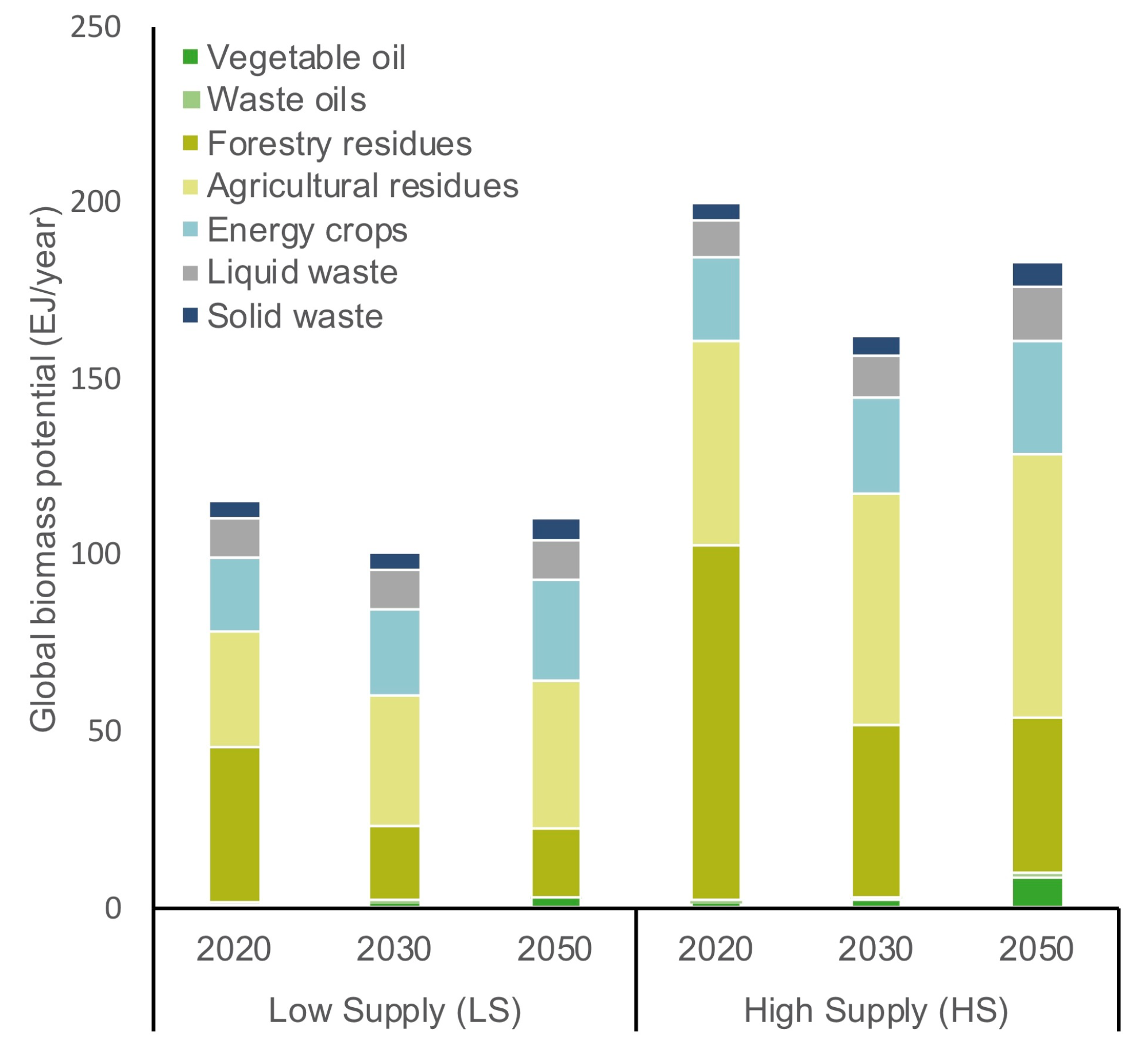
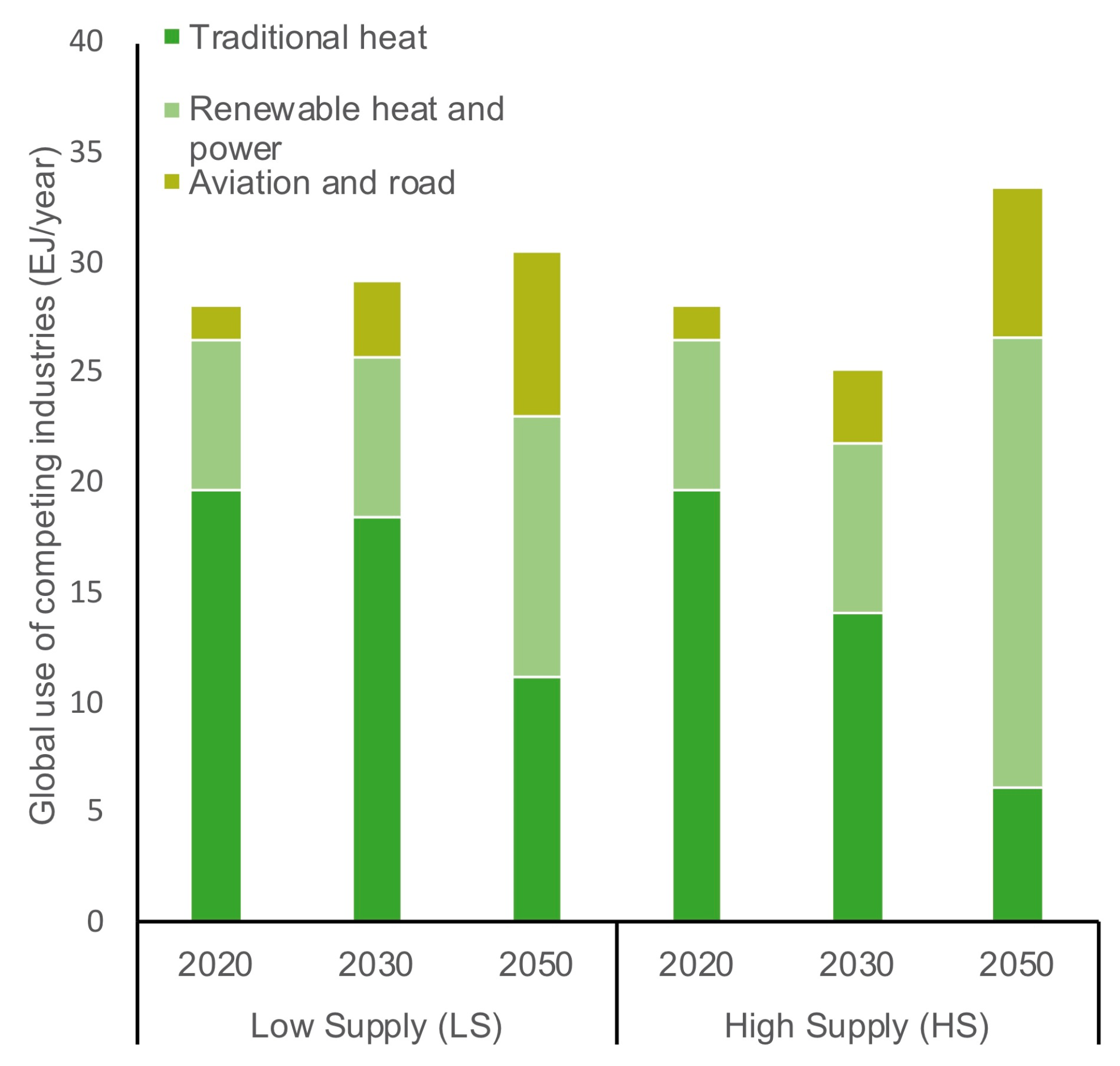
2.2.1. Biomass Supply Scenarios

In a study by De Jong et al. [9], the amount of available biomass in the EU to supply the aviation sector was analyzed. He indicated that there is uncertainty embedded in the determination of domestic availability and import potential of biomass. To capture this uncertainty, De Jong et al. [9] developed several supply and demand scenario. Although on a broader spatial scale, this study uses a similar approach. Low Supply (LS) and High Supply (HS) scenarios are developed based on feedstock availability and competing industries. In the LS scenario, a conservative estimation of biomass availability is combined with high competition from other industries. In the HS scenario a more optimistic view on biomass availability is combined with less competition from other industries. In order to determine the amount of biomass available for the production of marine biofuels, firstly, the domestic availability of each feedstock category in each region is estimated by means of a comprehensive literature review [9,15,16,17,18,19,20]. The resulting biomass availability estimates are shown in Figure 2.

Secondly, potential competing users are identified and deducted from domestic biomass availability. Competing users of biomass can be visualized as a cascade in which some sectors create more value out of products than others. Therefore, the use of biomass by other sectors such as aviation and automotive should be deducted from the availability. The estimated competing users are shown in Figure 3.

Lastly, the remaining amount of biomass is considered to be available for the production of marine biofuels.

2.2.2. Biofuel Demand Scenarios

Forecasting marine biofuel demand consists of two aspects. Firstly, the development of absolute energy demand from the shipping sector needs to be considered. In this study, three of the IMO scenarios are used to estimate future energy demand from the shipping industry. These scenarios are further referred to as Low Demand (LD), Base Demand (BD) and High Demand (HD).

Secondly, the share of biofuels in the future energy mix should be estimated and also specified per region. While energy demand from shipping is driven by global GDP and growth of seaborne trade, demand for marine biofuels is mainly driven by drivers of general eco-innovation [21]. Within drivers of general eco-innovation, regulatory incentives are arguably the key drivers for the implementation of marine biofuels. This is mainly because bio-energy technologies are not yet financially competitive with fossil fuels [22].

Three possible future policy scenarios are developed. In the Europe scenario, it is assumed that shipping is included in the RED II and, thus, complies with these targets. In the Most-Likely (ML) scenario, leading countries in the field of sustainability are expected to comply with the RED II targets. In the World scenario, all countries are expected to comply with the IMO targets of 50% GHG reduction by 2050 compared to 2008 levels. The resulting amount of biofuel for compliance is visualized in Figure 4. Figure 4 only shows the Base Demand (BD) scenario. It can be observed from Figure 4 that compliance with the IMO targets is a significant task.

2.3. Model Parameters

In order to simulate the various supply and demand scenarios using the developed optimization model, several parameters are required. These parameters can be categorized into economic, environmental and technological parameters.

2.3.1. Economic Parameters

Economic parameters consist of feedstock, transport, processing and upgrading costs. Costs for all feedstock categories per region were estimated as follows. For vegetable and waste oils, market-based prices were used. Agricultural and forestry residues are both considered waste streams; therefore, their production costs are assumed to be zero [23]. However, there are costs associated with the collection and field transport of these feedstocks [24]. For Europe, values from Hoogwijk and Graus [20], De Wit and Faaij [24], Allen et al. [25] and Ericsson et al. [26] are used. Since the costs for both agricultural and forestry residues are dominated by collection and field transport, the costs in Europe are scaled with a combination of regional labor costs and gasoline prices to obtain values for all other regions.

For lignocellulosic energy crops, costs of perennial grasses from Ericsson et al. [26] are used for Europe. De Wit and Faaij [24] stated that factors that dominate the costs of energy crops are land costs, wage level and production efficiency. Therefore, the base costs of energy crops are scaled with regional labor costs and gasoline prices. Liquid wastes and solid wastes are considered as residue streams. In contrast to agricultural and forestry residues, these waste types can be collected in centralized waste collection plants. This causes gathering and transport costs to be zero.

Hoogwijk and Graus [20] estimated costs of residues and energy crops for all world regions. However, they found residue prices to be uncertain. As an example, they indicated residue prices in OECD Europe to be between 0.9 and 10.5 EUR/GJ, which is an extremely large range. Alves et al. [27] states that “Biomass feedstock cost plays a major impact in the operational costs of a plant and the uncertainty associated with the feedstock supply is the most critical aspect of bio-refineries profitability”. Hence, feedstock costs have a significant contribution to refinery operating costs but are simultaneously uncertain. Therefore, feedstock costs should be further studied in the sensitivity analysis. Since a two-stage supply chain is considered, costs for processing and upgrading are separated and visualized in Figure 5.

2.3.2. Environmental Parameters

Analogous to the economic parameters, emission factors can be assigned to different life-cycle phases of the end product. To determine the allocation of GHG emissions to the life-cycle of the fuel, the method of the RED II is used. For the cultivation of feedstocks, default values from the RED II were used. Emission factors related to processing and upgrading of the fuel were obtained from the RED II and a Life-Cycle Analysis (LCA) of De Jong et al. [47].

Unit emissions for transport were taken from McKinnon and Piecyk [48]. Unit emissions from sea transport are highly dependent on the vessel type, trade route, and corresponding vessel utilization rate. For short-sea and deep-sea shipping, average emission factors of 16 and 12 gCO${}_2$-eq/ton-km are used, respectively [48].

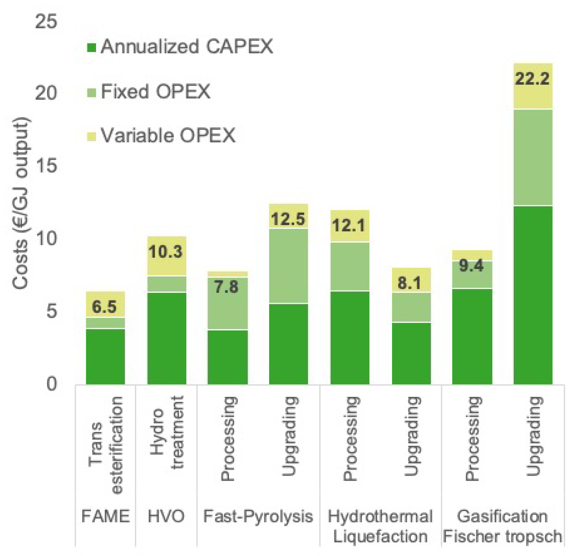
2.3.3. Technological Parameters

Process yields are defined as the amount of biofuel that can be produced from a certain quantity of biomass. In this case, two conversion yields are of importance: the yield from biomass to the bio-intermediate and the yield from the bio-intermediate to the biofuel end product. Conversion yields are dependent on the process conditions and the molecular composition of feedstocks. For example, grain residues have a high ash content which can reduce its conversion yield [30]. Examples of process conditions that can affect the yields are temperature, solvent-to-feedstock ratio (for fast pyrolysis) and the fluidizing medium (for GFT) [30]. In order to obtain a realistic estimation of these process yields, an average is taken from the values of different literature sources. The resulting values are visualized in Figure 6.

3. Results

In this section, the results from simulating the proposed supply and demand scenario using the developed MILP model are displayed. Results can be subdivided into three categories. Firstly, cost and emission projections associated with the large scale use of marine biofuels are depicted. This also includes the marginal costs of GHG reduction. Secondly, the most feasible deployment of various feedstock and conversion technology combinations is shown. Lastly, the most feasible trade flows of the intermediate bio-energy carriers and biofuels are elaborated upon. These results give an impression of the expected export and import regions of biomass and biofuel.

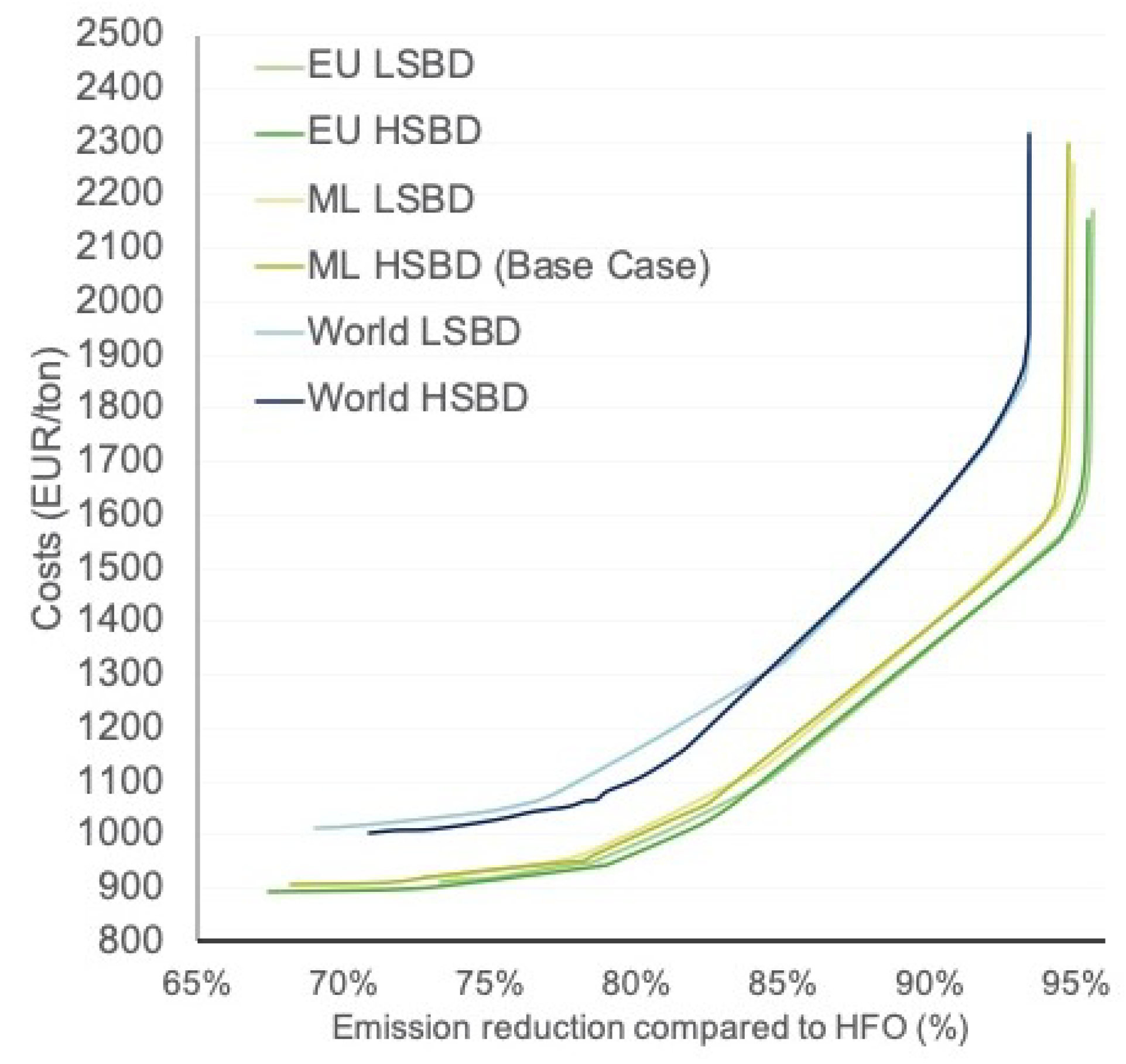
3.1. Costs Versus Emissions

The multi-objective optimization induces a trade-off between costs and emissions. The resulting marginal costs of GHG reduction for all scenarios are visualized in Figure 7. In every run, this trade-off is reconsidered to reach the highest GHG reduction against the lowest costs. A clear trade-off between costs and emission reduction is visualized. The most beneficial trade-off is found to be around 80% GHG reduction compared to Heavy Fuel Oil (HFO), which corresponds to the average fuel costs of around 900–1050 EUR/ton of biofuel.

In Figure 8, the average fuel costs per time period are displayed. These costs are obtained by dividing the total expenses of that time period by the amount of fuel produced during that time period. It should be noted that these are average costs; in reality, different costs would be allocated to different fuel types. It stands out that, at first, fuel costs decline as a result of scale advantages and the use of cheaper feedstocks. However, after a strong decrease, costs gradually go up again. Rising demand induces the need for feedstocks that are increasingly difficult to collect, driving up the feedstock costs.

The results showed that around 20% of the costs are related to the raw materials, and 50% of the costs are associated with the production of the intermediate bio-energy carrier. The remaining 30% is related to the upgrading process. On the contrary, the upgrading process is responsible for around 85% of total GHG emissions. This is a result of the generous amounts of hydrogen required for the upgrading process. It is assumed that the used hydrogen originates from fossil sources. Using hydrogen from the of-gasses of the process or sourcing green hydrogen would make an enormous impact on the GHG reduction potential of drop-in biofuels. Additionally, it could be argued if drop-in biofuels for marine purposes require vast amounts of upgrading. Marine engines are often built for heavy-duty operations and residual or low quality fuel.

3.2. Technology and Feedstock Deployment

A total of five drop-in biofuel production pathways were considered in this study. In the first time period, only FAME and HVO were considered to be commercially available. After 2025, Fast-Pyrolysis (FP) and Gasification Fischer–Tropsch (GFT) were introduced. Hydrothermal Liquefaction (HTL) was introduced after 2030.

In all studied scenarios, HTL showed to be the most promising fuel both on economic and environmental performance. The main causes for this are the minor amount of upgrading required compared to Fast-Pyrolysis and the possibility in using a wide variety of feedstocks, including manure and sludges. However, the potential of HTL could be inhibited by its low TRL (Technology Readiness Level).

Feedstock deployment resulted in a mix of feedstocks, with a small preference for the use of agricultural residues. The reason for this mix can be partly attributed to the existing trade-off between costs, environmental performance and technological efforts [54]. As an example, waste streams such as manure and Municipal Solid Waste (MSW) are cheap and have a high emission reduction potential. However, it is extremely difficult to obtain a constant stream that is suitable for the production of biofuel with steady quality. For residues from agricultural and forestry practices, feedstock costs rise when demand increases due to the need for feedstocks that become increasingly difficult to collect.

In Figure 9, the enormous refinery capacities required to reach the proposed targets are lined up for the three geographical demand scenarios. To place this in perspective, common biorefinery sizes mentioned in the literature are in the range of 1000–2000 dry ton input per day. This would correspond to an estimated biorefinery output of 0.0035–0.007 EJ/yr (using an average feedstock energy density of 18 MJ/kg and conversion yield of 0.6). In order to comply with the GHG reduction target of the IMO by 2050, this would impose a required investment in the range of 1100–2200 new biorefineries of that size worldwide during the studied time period. This provides an idea of the enormous challenges that lie ahead.

3.3. Trade Flows

Lastly, after the determination of the spatial distributions of future marine biofuel demand and feedstock availability, imbalances in supply and demand are found. Especially in the first time period, when oils and fats are the only usable feedstocks, significant imbalances exist. This is confirmed by a large amount of trade in vegetable and waste oils. The MILP model developed in this study assumes that biomass is converted to an intermediate bio-energy carrier before it is transported between regions. Hence, a distinction can be made between the trade of the intermediate bio-energy carrier and trade of the biofuel end-product.

Figure 10 displays the most feasible exports and imports of the intermediate product between regions. The exporting regions can also be identified as the biomass exporting regions, seeing that the processing step is always performed in the domestic region. In the Europe scenario, a large difference between the LS and HS scenarios exist. This is mainly caused by the increased availability of oils and fats in the HS scenario. This causes Northern America to gain more export opportunities, which is mainly caused by less competition from the road and aviation sector for these feedstocks in this scenario.

In the Most-Likely scenario, Eastern Asia and Southern Asia are the major suppliers of the intermediate product. In the World scenario, Southern Asia is the dominant exporter, which is mainly caused by the large availability of animal manure in that region. Despite the large technological efforts associated with the conversion of this feedstock, the model chooses to use this feedstock for the production of biofuels.

On the other side, intermediate imports are more centralized. These importing regions are relatively constant and are highly dependent on the spatial distribution of fuel demand. In the European scenario, Western Europe and Southern Europe are expected to import intermediate products. In the ML scenarios, Northern America is included in this group. In the World scenario, a shift in demand causes Asian regions to become the main importers.

Exports and imports of biofuels are displayed in Figure 11. From this figure, it can be observed that biofuel exports are dominated by Southern Europe in the Europe and ML scenario. Hence, Southern Europe is considered the most preferable spot to construct biorefineries. This is mainly caused by its central location and beneficial local operating costs. Elements such as available infrastructure and local subsidies for attracting this type of business have not been taken into account.

Figure 11 shows that importing regions of biofuel are more diverse. In these importing regions, a shortage on refinery capacity results in the need for imports. In the European scenario, most biofuels are imported to Western and Northern Europe. In the ML scenario, Northern America also imports a fair share of biofuel. The importing regions of biofuel in the World scenario are somewhat more distributed. The large share of South Eastern Asia can be dedicated to the presence of Singapore in that area, which on its own is responsible for around 20% of global fuel sales.

4. Conclusions

In this study, the potential of drop-in biofuels for the maritime industry was assessed. In order to measure this potential, a strategic supply chain optimization was performed to determine the economic and environmental performance of drop-in biofuels. Additionally, a comprehensive scenario analysis identified the availability of biomass and the required investments in new infrastructure and technologies to achieve the proposed GHG reduction targets of the RED II and IMO.

Concerning the economic performance of drop-in biofuels, the price gap with fossil products is still large. Although technological learning effects were not considered, the production costs of drop-in biofuel were projected to initially decrease. This is mainly caused by the gradually growing influence of economies of scale in combination with the introduction of new technologies that are able to use cheaper feedstocks. However, drop-in biofuels could also be the victim of their own success. In contrast to other renewable fuels, increasing demand results in the need for more expensive feedstocks that are difficult to collect.

The possible GHG reduction potential of drop-in biofuels was found to be between 68 and 95% compared to HFO for a cost of 850–2300 EUR/ton. Emission reductions of 80% compared to HFO are estimated to be achieved at fuel costs of around 900–1050 EUR/ton.

The availability of oils and fats is a severe barrier to the scalability of drop-in biofuels. Additionally, it could be argued if dependency on waste oils for the production of marine fuels is desirable. This increases the urgency for the rapid development of new conversion technologies that pave the road for the usage of more abundant feedstocks. It has been shown that in order to achieve the proposed emission reduction targets, enormous investments in new biorefineries are required. This entails investments in smaller processing facilities located near the feedstock source and larger refinery hubs located near ports.

In conclusion, drop-in biofuels offer a significant GHG reduction potential for the shipping industry. These fuels can be used without adaptations to existing fuel infrastructure. FAME and HVO are already commercially available, but limited feedstock availability induces the need for investments in new conversion technologies. When these technologies become available, enough biomass is domestically available to serve a large part of the shipping industry.

References

1. Tyrovola, T.; Dodos, G.; Kalligeros, S.; Zannikos, F. The introduction of biofuels in marine sector. J. Environ. Sci. Eng. A 2017, 6, 415–421. [Google Scholar] [CrossRef]
2. EU. Reducing Emissions from the Shipping Sector. Available online: https://ec.europa.eu/clima/policies/transport/shipping_en (accessed on 11 March 2021).
3. McGill, R.; Remley, W.; Winther, K. Alternative Fuels for Marine Applications; A Report from the IEA Advanced Motor Fuels Implementing Agreement; Publications Office of the European Union: Luxembourg, 2013; Volume 54. [Google Scholar]
4. Moirangthem, K.; Baxter, D. Alternative Fuels for Marine and Inland Waterways; European Commission: Brussels, Belgium, 2016. [Google Scholar]
5. Czermanski, E.; Cirella, G.; Oniszczuk-Jastrzabek, A.; Pawlowska, B.; Notteboom, T. An Energy Consumption Approach to Estimate Air Emission Reductions in Container Shipping. Energies 2021, 14, 278. [Google Scholar] [CrossRef]
6. Van Vliet, O.P.; Faaij, A.P.; Turkenburg, W.C. Fischer–Tropsch diesel production in a well-to-wheel perspective: A carbon, energy flow and cost analysis. Energy Convers. Manag. 2009, 50, 855–876. [Google Scholar] [CrossRef]
7. Bouman, E.A.; Lindstad, E.; Rialland, A.I.; Strømman, A.H. State-of-the-art technologies, measures, and potential for reducing GHG emissions from shipping—A review. Transp. Res. Part D Transp. Environ. 2017, 52, 408–421. [Google Scholar] [CrossRef]
8. Sustainable Shipping Initiative. The Role of Sustainable Biofuels in the Decarbonisation of Shipping; Technical Report; Sustainable Shipping Initiative, SSI: London, UK, 2019. [Google Scholar]
9. De Jong, S.; van Stralen, J.; Londo, M.; Hoefnagels, R.; Faaij, A.; Junginger, M. Renewable jet fuel supply scenarios in the European Union in 2021–2030 in the context of proposed biofuel policy and competing biomass demand. GCB Bioenergy 2018, 10, 661–682. [Google Scholar] [CrossRef]
10. Forsberg, G. Biomass energy transport: Analysis of bioenergy transport chains using life cycle inventory method. Biomass Bioenergy 2000, 19, 17–30. [Google Scholar] [CrossRef]
11. Mankowska, M.; Plucinski, M.; Kotowska, I. Biomass Sea-Based Supply Chains and the Secondary Ports in the Era of Decarbonization. Energies 2021, 14, 1796. [Google Scholar] [CrossRef]
12. Lin, T.; Rodríguez, L.F.; Shastri, Y.N.; Hansen, A.C.; Ting, K.C. GIS-enabled biomass-ethanol supply chain optimization: Model development and Miscanthus application. Biofuels Bioprod. Biorefining 2013, 7, 314–333. [Google Scholar] [CrossRef]
13. Giarola, S.; Zamboni, A.; Bezzo, F. Spatially explicit multi-objective optimisation for design and planning of hybrid first and second generation biorefineries. Comput. Chem. Eng. 2011, 35, 1782–1797. [Google Scholar] [CrossRef]
14. Smith, T.W.P.; Jalkanen, J.P.; Anderson, B.A.; Corbett, J.J.; Faber, J.; Hanayama, S.; O’Keeffe, E.; Parker, S.; Johansson, L.; Aldous, L.; et al. Third IMO Greenhouse Gas Study 2014; International Maritime Organization (IMO): London, UK, 2014; p. 327. [Google Scholar] [CrossRef] [Green Version]
15. Nakada, S.; Saygin, D.; Gielen, D. Global Bioenergy Supply and Demand Projections; A Working Paper for REmap 2030; IRENA: Tokyo, Japan, 2014. [Google Scholar]
16. Leguijt, C. Bio-Scope. 2020. Available online: https://ce.nl/wp-content/uploads/2021/03/CE_Delft_190186_Bio-Scope_Def.pdf (accessed on 20 August 2021).
17. Daioglou, V.; Doelman, J.C.; Wicke, B.; Faaij, A.; van Vuuren, D.P. Integrated assessment of biomass supply and demand in climate change mitigation scenarios. Glob. Environ. Chang. 2019, 54, 88–101. [Google Scholar] [CrossRef] [Green Version]
18. Smeets, E.M.; Faaij, A.P.; Lewandowski, I.M.; Turkenburg, W.C. A bottom-up assessment and review of global bio-energy potentials to 2050. Prog. Energy Combust. Sci. 2007, 33, 56–106. [Google Scholar] [CrossRef] [Green Version]
19. Gregg, J.S.; Smith, S.J. Global and regional potential for bioenergy from agricultural and forestry residue biomass. Mitig. Adapt. Strateg. Glob. Chang. 2010, 15, 241–262. [Google Scholar] [CrossRef]
20. Hoogwijk, M.; Graus, W. Global Potential of Renewable Energy Sources: A Literature Assessment; Background Report Prepared by Order of REN21; Ecofys: Utrecht, The Netherlands, 2008. [Google Scholar]
21. Aronietis, R.; Sys, C.; van Hassel, E.; Vanelslander, T. Forecasting port-level demand for LNG as a ship fuel: The case of the port of Antwerp. J. Shipp. Trade 2016, 1, 2. [Google Scholar] [CrossRef] [Green Version]
22. Hsieh, C.; Felby, C. Biofuels for the Marine Shipping Sector; IEA Bioenergy: Paris, France, 2017. [Google Scholar]
23. De Wit, M.; Faaij, A. European biomass resource potential and costs. Biomass Bioenergy 2010, 34, 188–202. [Google Scholar] [CrossRef]
24. De Wit, M.; Faaij, A. Biomass Resources Potential and Related Costs; Refuel Work Package 3; Copernicus Institute: Utrecht, The Netherlands, 2008. [Google Scholar]
25. Allen, J.; Browne, M.; Hunter, A.; Boyd, J.; Palmer, H. Logistics management and costs of biomass fuel supply. Int. J. Phys. Distrib. Logist. Manag. 1998, 28, 463–477. [Google Scholar] [CrossRef]
26. Ericsson, K.; Rosenqvist, H.; Nilsson, L.J. Energy crop production costs in the EU. Biomass Bioenergy 2009, 33, 1577–1586. [Google Scholar] [CrossRef] [Green Version]
27. Alves, C.M.; Valk, M.; De Jong, S.; Bonomi, A.; van der Wielen, L.A.; Mussatto, S.I. Techno-economic assessment of biorefinery technologies for aviation biofuels supply chains in Brazil. Biofuels Bioprod. Biorefining 2017, 11, 67–91. [Google Scholar] [CrossRef]
28. Swanson, R.M.; Platon, A.; Satrio, J.; Brown, R.; Hsu, D.D. Techno-Economic Analysis of Biofuels Production Based on Gasification; Technical Report; National Renewable Energy Lab. (NREL): Golden, CO, USA, 2010. [Google Scholar]
29. Rafati, M.; Wang, L.; Dayton, D.C.; Schimmel, K.; Kabadi, V.; Shahbazi, A. Techno-economic analysis of production of Fischer-Tropsch liquids via biomass gasification: The effects of Fischer-Tropsch catalysts and natural gas co-feeding. Energy Convers. Manag. 2017, 133, 153–166. [Google Scholar] [CrossRef] [Green Version]
30. Tanzer, S. Plant+ Boom= Boat+ Vroom: A Comparative Technoeconomic and Environmental Assessment of Marine Biofuel Production in Brazil and Scandinavia Using Residual Lignocellulosic Biomass and Thermochemical Conversion Technologies. 2017. Available online: http://resolver.tudelft.nl/uuid:ac21de73-e747-479d-b6e3-5e2b4e7bb88d (accessed on 20 August 2021).
31. Cornelio da Silva, C. Techno-Economic and Environmental Analysis of Oil Crop and Forestry Residues based Biorefineries for Biojet Fuel Production in Brazil. 2016. Available online: http://resolver.tudelft.nl/uuid:1dd8082f-f4a5-4df6-88bb-e297ed483b54 (accessed on 20 August 2021).
32. Zhu, Y.; Biddy, M.J.; Jones, S.B.; Elliott, D.C.; Schmidt, A.J. Techno-economic analysis of liquid fuel production from woody biomass via hydrothermal liquefaction (HTL) and upgrading. Appl. Energy 2014, 129, 384–394. [Google Scholar] [CrossRef]
33. Atsonios, K.; Kougioumtzis, M.A.; Panopoulos, K.D.; Kakaras, E. Alternative thermochemical routes for aviation biofuels via alcohols synthesis: Process modeling, techno-economic assessment and comparison. Appl. Energy 2015, 138, 346–366. [Google Scholar] [CrossRef]
34. Sarkar, S.; Kumar, A.; Sultana, A. Biofuels and biochemicals production from forest biomass in Western Canada. Energy 2011, 36, 6251–6262. [Google Scholar] [CrossRef]
35. Anex, R.P.; Aden, A.; Kazi, F.K.; Fortman, J.; Swanson, R.M.; Wright, M.M.; Satrio, J.A.; Brown, R.C.; Daugaard, D.E.; Platon, A.; et al. Techno-economic comparison of biomass-to-transportation fuels via pyrolysis, gasification, and biochemical pathways. Fuel 2010, 89, S29–S35. [Google Scholar] [CrossRef]
36. AlNouss, A.; McKay, G.; Al-Ansari, T. A comparison of steam and oxygen fed biomass gasification through a techno-economic-environmental study. Energy Convers. Manag. 2020, 208, 112612. [Google Scholar] [CrossRef]
37. Tzanetis, K.F.; Posada, J.A.; Ramirez, A. Analysis of biomass hydrothermal liquefaction and biocrude-oil upgrading for renewable jet fuel production: The impact of reaction conditions on production costs and GHG emissions performance. Renew. Energy 2017, 113, 1388–1398. [Google Scholar] [CrossRef]
38. Jones, S.B.; Meyer, P.A.; Snowden-Swan, L.J.; Padmaperuma, A.B.; Tan, E.; Dutta, A.; Jacobson, J.; Cafferty, K. Process Design and Economics for the Conversion of Lignocellulosic Biomass to Hydrocarbon Fuels: Fast Pyrolysis and Hydrotreating Bio-Oil Pathway; Technical Report; Pacific Northwest National Lab. (PNNL): Richland, WA, USA, 2013. [Google Scholar]
39. Magdeldin, M.; Kohl, T.; Järvinen, M. Techno-economic assessment of the by-products contribution from non-catalytic hydrothermal liquefaction of lignocellulose residues. Energy 2017, 137, 679–695. [Google Scholar] [CrossRef]
40. Tews, I.J.; Zhu, Y.; Drennan, C.; Elliott, D.C.; Snowden-Swan, L.J.; Onarheim, K.; Solantausta, Y.; Beckman, D. Biomass Direct Liquefaction Options. TechnoEconomic and Life Cycle Assessment; Technical Report; Pacific Northwest National Lab. (PNNL): Richland, WA, USA, 2014. [Google Scholar]
41. Wright, M.M.; Daugaard, D.E.; Satrio, J.A.; Brown, R.C. Techno-economic analysis of biomass fast pyrolysis to transportation fuels. Fuel 2010, 89, S2–S10. [Google Scholar] [CrossRef] [Green Version]
42. Meyer, P.A.; Snowden-Swan, L.J.; Rappé, K.G.; Jones, S.B.; Westover, T.L.; Cafferty, K.G. Field-to-fuel performance testing of lignocellulosic feedstocks for fast pyrolysis and upgrading: Techno-economic analysis and greenhouse gas life cycle analysis. Energy Fuels 2016, 30, 9427–9439. [Google Scholar] [CrossRef]
43. Brown, T.R.; Thilakaratne, R.; Brown, R.C.; Hu, G. Techno-economic analysis of biomass to transportation fuels and electricity via fast pyrolysis and hydroprocessing. Fuel 2013, 106, 463–469. [Google Scholar] [CrossRef] [Green Version]
44. Shemfe, M.B.; Gu, S.; Ranganathan, P. Techno-economic performance analysis of biofuel production and miniature electric power generation from biomass fast pyrolysis and bio-oil upgrading. Fuel 2015, 143, 361–372. [Google Scholar] [CrossRef] [Green Version]
45. Meyer, P.A.; Snowden-Swan, L.J.; Jones, S.B.; Rappé, K.G.; Hartley, D.S. The effect of feedstock composition on fast pyrolysis and upgrading to transportation fuels: Techno-economic analysis and greenhouse gas life cycle analysis. Fuel 2020, 259, 116218. [Google Scholar] [CrossRef]
46. Landälv, I.; Waldheim, L.; van den Heuvel, E.; Kalligeros, S. Building up the Future Cost of Biofuel; European Comission, Sub Group on Advanced Biofuels: Brussels, Belgium, 2017. [Google Scholar]
47. De Jong, S.; Antonissen, K.; Hoefnagels, R.; Lonza, L.; Wang, M.; Faaij, A.; Junginger, M. Life-cycle analysis of greenhouse gas emissions from renewable jet fuel production. Biotechnol. Biofuels 2017, 10, 64. [Google Scholar] [CrossRef] [Green Version]
48. McKinnon, A.; Piecyk, M. Measuring and Managing CO2 Emissions; European Chemical Industry Council: Edinburgh, UK, 2010. [Google Scholar]
49. Han, D.; Yang, X.; Li, R.; Wu, Y. Environmental impact comparison of typical and resource-efficient biomass fast pyrolysis systems based on LCA and Aspen Plus simulation. J. Clean. Prod. 2019, 231, 254–267. [Google Scholar] [CrossRef]
50. Oasmaa, A.; Kuoppala, E.; Gust, S.; Solantausta, Y. Fast pyrolysis of forestry residue. 1. Effect of extractives on phase separation of pyrolysis liquids. Energy Fuels 2003, 17, 1–12. [Google Scholar] [CrossRef]
51. Buah, W.; Cunliffe, A.; Williams, P. Characterization of products from the pyrolysis of municipal solid waste. Process Saf. Environ. Prot. 2007, 85, 450–457. [Google Scholar] [CrossRef]
52. Sipra, A.T.; Gao, N.; Sarwar, H. Municipal solid waste (MSW) pyrolysis for bio-fuel production: A review of effects of MSW components and catalysts. Fuel Process. Technol. 2018, 175, 131–147. [Google Scholar] [CrossRef]
53. Mullen, C.A.; Boateng, A.A. Chemical composition of bio-oils produced by fast pyrolysis of two energy crops. Energy Fuels 2008, 22, 2104–2109. [Google Scholar] [CrossRef]
54. El Takriti, S.; Pavlenko, N.; Searle, S. Mitigating International Aviation Emissions: Risks and Opportunities for Alternative Jet Fuels. 2017. Available online: https://theicct.org/sites/default/files/publications/Aviation-Alt-Jet-Fuels_ICCT_White-Paper_22032017_vF.pdf (accessed on 20 August 2021).
Figure 1. Schematic representation of the modeled supply chain.
Sustainability 13 09900 g001
Figure 2. Estimated biomass availability per feedstock for the Low Supply (LS) and High Supply (HS) scenarios.
Sustainability 13 09900 g002
Figure 3. Estimated biomass use of competing industries for the two supply scenarios.
Sustainability 13 09900 g003
Figure 4. Required amount of biofuel to comply with the set targets for the different scenarios. Only the Base Demand (BD) scenario is shown. This assumes that only biofuels and LNG are used to comply with these targets.
Sustainability 13 09900 g004
Figure 5. Processing and upgrading costs for different technologies. Data from [9,28,29,30,31,32,33,34,35,36,37,38,39,40,41,42,43,44,45,46,46].
Sustainability 13 09900 g005
Figure 6. Conversion yields for different technologies. Data from [28,29,30,31,32,33,34,37,38,39,41,42,43,44,45,46,49,50,51,52,53,30].
Sustainability 13 09900 g006
Figure 7. Marginal costs of Green House Gas reduction compared to HFO. A Well-to-Wake emission factor of 87.5 gCO 2 -eq/MJ for HFO was used.
Sustainability 13 09900 g007
Figure 8. Projected average biofuel costs over the studied time period.
Sustainability 13 09900 g008
Figure 9. Required bio-refinery capacity per region to comply with the targets proposed in the developed scenarios. Capacity is given in the required refinery output. Integers represent the studied time intervals. 1: 2020–2025; 2: 2025–2030; 3: 2030–2035; 4: 2035–2040; 5: 2040–2045; 6: 2045–2050.
Sustainability 13 09900 g009
Figure 10. Intermediate bio-energy carrier exports and imports per region for all studied scenarios during the entire time period.
Sustainability 13 09900 g010
Figure 11. Biofuel exports and imports per region for all studied scenarios during the entire time period.
Sustainability 13 09900 g011