Abstract
Renewable energy is produced using renewable natural resources, including wind power. The Taiwan government aims to have renewable energy account for 20% of its total power supply by 2025, in which offshore wind power plays an important role. This paper explores the application of index insurance to renewable energy for offshore wind power in Taiwan. We employ autoregressive integrated moving average models to forecast power generation on a monthly and annual basis for the Changhua Demonstration Offshore Wind Farm. These predictions are based on an analysis of 39 years of hourly wind speed data (1980–2018) from the Modern-Era Retrospective analysis for Research and Applications, Version 2, of the National Aeronautics and Space Administration. The data analysis and forecasting models describe the methodology used to design the insurance contract and its index for predicting offshore wind power generation. We apply our forecasting results to insurance contract pricing.
1. Introduction
The rise in CO2 emissions over the past 30 years and the growing global demand for stable electricity present a global challenge. Growth in renewable energy generation is crucial to meeting the 2050 targets for greenhouse gas reduction under the Paris Agreement [1]. Within the United Nations Framework Convention on Climate Change, the Paris Agreement, also called the Paris Climate Agreement, was adopted in December 2015. The aim of this international treaty is to curb greenhouse gas emissions and global warming—specifically, to limit the global temperature increase in the 21st century to 2 °C above preindustrial levels, and even further, to 1.5 °C above preindustrial levels. To achieve this goal, the parties aim to reach the global peak of greenhouse gas emissions as soon as possible and achieve a climate-neutral world by 2050. In June 2015, in response to the global consensus on mitigating the greenhouse effect, Taiwan passed the Greenhouse Gas Reduction and Management Act, which sets targets for reducing Taiwan’s greenhouse gas emissions to below 50% of 2005 levels by 2050. Because energy-related challenges differ by country, each country must develop its own energy model for facilitating a transition to a low-carbon economy.
In recent years, many countries and territories, including Taiwan, have begun installing offshore wind farms. Of the considerable number of offshore wind farms under planning in Taiwan, some are under active development to meet the island’s ambitious target of generating 20% of its electricity from renewable power by 2025. According to the Bureau of Energy of Taiwan’s Ministry of Economic Affairs, the total power supply was 55.79 GW in November 2019. Government policy plans to phase out nuclear power plants and have natural gas, coal, and renewable energy (such as solar PV, offshore wind power, etc.) account for 50%, 30%, and 20%, respectively, of the total power supply by 2025. A target of an installed capacity of 5.7 GW for offshore wind power has been set for 2020 to 2025, and for 2026 to 2035, an additional generation capacity of approximately 10 GW has been planned. Thus, offshore wind power is expected to play a critical role in the coming decades.
Taiwan’s western sea areas have been rated as the world’s best offshore wind farm sites by 4C Offshore [2], an international consulting firm focused on offshore energy, with regard to wind power potential. Notably, 7 of the world’s 20 best sites in terms of wind power potential were located in the Taiwan Strait. To promote offshore wind power and attract experienced international developers to this region, a stable regulatory framework has been established, and 20-year power purchase agreements have been offered under the feed-in tariff (FIT) system. The FIT system entails fixed electricity prices paid to renewable energy producers for each unit of energy produced. Payment of the FIT is guaranteed for a certain period, which is often dependent on the economic lifetime of the renewable energy projects. These agreements provide a stable single-revenue stream to underlying energy prices.
Index insurance is an insurance design that does not indemnify pure losses but instead issues a claim payment in case of an objective triggering event. Payouts are made on the basis of an index or a set of indexes that are correlated to the risks associated with the insured. Specifically, data from specific weather stations or satellites are examined in such considerations. Interest in the use of index insurance has grown in recent decades [3,4]. Various projects are being piloted in low-income countries by the World Bank to mitigate losses attributable to natural disasters. The World Bank and its implementing partners have developed weather, area yield, and livestock index products for insuring crops and dairy cattle. Countries such as Ethiopia, Kenya, Malawi, and Mozambique have experimented with index-based insurance. The aim is to better manage weather risk, thereby enabling investment and growth in the agricultural sector for smallholder farmers. Index insurance is also a key component for many governments committed to realizing the Sustainable Development Goals (SDGs) [5] of the United Nations that center on addressing climate change and achieving food security to reduce poverty and vulnerability. This innovative approach has gradually become a tool for risk management, opening up a new range of possibilities and business opportunities for insurers closely attuned to new trends.
Weather risks can lead to poor yields and crop damage, resulting in lower or even no revenue for farmers. As its name suggests, weather index insurance covers weather-related risks. Based on meteorological conditions and indicators such as rainfall and temperature, it can prevent adverse selection and moral hazard problems as well as reduce transaction costs [6]. Weather index insurance constitutes an effective approach to managing natural disasters and climate change. Moreover, it is essential to agricultural development in emerging countries [7,8,9,10,11,12,13]. Unlike conventional insurance, index insurance does not necessarily require the services of claim assessors. Thus, the loss verification process can be bypassed, expediting the claim procedure in addition to reinforcing its objectivity. In protecting data from manipulation, index insurance can reduce the risk of adverse selection and prevent moral hazards, thereby minimizing risks incurred by the insurer and increasing confidence among market participants and policyholders alike [14,15].
Index insurance has been criticized because it is not based on the actual losses experienced by policyholders [10]. In index insurance, the principal challenge is basis risk, the risk under which the trigger index is imperfectly correlated with the underlying risk exposure. Index insurance is expected to insure against the loss of revenue or assets. Developing adequate index insurance entails minimizing the associated basis risk between the index-triggered payouts and the insured’s actual loss. Therefore, whether single or multiple, index values should be carefully identified and closely correlated with the insured’s losses in income or assets.
Although the principles of index insurance appear to reduce the costs associated with the risks of being uninsured by traditional insurance, in most index-based projects, including crop yield insurance, stochastic income streams are insured [7]. Many index insurance projects are based on weather indexes, depending on the data availability and its correlations with losses [16]. Applications of index insurance in the renewable energy sector are rare. By contrast, several studies have addressed such applications in the agricultural sector. The indexes used can measure weather risks, such as drought or extreme temperature highs, to protect production outcomes. In this regard, the payouts are based on triggers correlated with yield losses [17,18,19,20,21].
Although wind is a source of clean energy, wind power generation is characterized by fluctuations because of the changeable nature of wind speed [22]. Given that the outputs of offshore wind farms are considerably influenced by wind speed, identifying locations where wind speeds are high and steady is crucial. Managing volatility risk in offshore wind power is critical because forecasting power generation in offshore wind projects is challenging. Investors and lenders must understand the impacts of wind conditions on project value in examining an asset for bankability, defined as their willingness to finance an offshore wind project at a reasonable return or interest rate. The decision to invest is typically taken once a certain level of confidence is reached, and suitable contractual risk coverage is in place. A bankable offshore wind project must have accurate power generation forecasts that directly address the financial aspects of predictable cash flows and reliable revenue streams to reassure investors and lenders.
In Taiwan, most lenders have limited experience and capacity to underwrite offshore wind projects. Therefore, project developers must demonstrate the availability and commitment of permanent financing in order for lenders to consider financing at an early stage. In order to encourage lenders to take on more offshore wind deals, the purpose of this study for index insurance applications focuses on helping lenders remove as much risk on the production volatility as possible. It is not practical to expect that lenders will suddenly start providing more financing for offshore wind projects with this insurance product but go back to the basic underwriting standards. Instead, we hope this insurance design can reduce the concerns of the volatility of renewable energy production from lenders’ point of view.
Because weather conditions can be quantified and indexed, the same concepts are applied in this study to create an index-based solution for mitigating risks involved in offshore wind power. We use the dependence structure between offshore wind power generation and weather indexes.
The exceedance probability is introduced to analyze the renewable energy industry. For example, wind speed at a particular wind farm is examined to characterize the uncertainty in wind power generation [23]. In the context of energy generation, developers and investors can apply exceedance probability to forecasting and business plan assumptions. Furthermore, lenders and insurers can use it to quantify the risk profile of individual offshore wind farms. In this regard, estimating the annual energy production (AEP) is pivotal. The AEP of an offshore wind farm is the total amount of electrical energy it produces over a year, measured in megawatt hours (MWh).
Wind power forecast corresponds with an estimate of the expected production of an offshore wind farm in the near future. Depending on the intended application, forecasting of wind power generation can be considered by different time scales. Long-term forecasting measured in years focuses on project feasibility analysis and planning for a specific site. Short-term forecasting concentrates on benefits during a wind farm’s operational period, measured in hours or days ahead for grid operators to schedule the economically efficient generation to meet the electrical demand. There are generally three forecasting approaches for wind power: the physical approach, the statistical approach, and the hybrid approach. More comprehensive literature reviews can be found in [24,25,26,27,28].
The physical approach based on weather data has been developed, downscaling the numerical weather prediction (NWP) data to describe the farm site, such as temperature and atmospheric conditions. However, these variables require large computational systems to achieve accurate wind speed forecasting and wind power predictions. On the other hand, the statistical approach needs vast data such as wind speed, wind direction, and temperature to analyze wind power and extract the statistical inference inside the time series of the previous power data itself. Thus, the link between historical power production and weather is determined and used to forecast the future power output. The hybrid approach is a combination of the physical and statistical approaches. Developing an index that should be easily measurable, objective, transparent, and independently verifiable [15] requires a time series dataset [29]. Compared with the physical forecast methods that depend on the input used in complex mathematical models, this study uses flexible time series forecasting, and the technique is easier to implement. By employing 39 years of hourly wind speed data (1980–2018) obtained from the Modern-Era Retrospective Analysis for Research and Applications, Version 2 (MERRA-2) of the National Aeronautics and Space Administration (NASA), we built autoregressive integrated moving average (ARIMA) models to forecast power generation at an offshore wind farm in Changhua, Taiwan, on a monthly and yearly basis. The results extend the understanding of the impacts of wind speed on the energy production of the offshore wind farm. We apply them in the formulation of the index insurance product, including the pricing model’s design. This insurance product is able to transfer wind volume risks to insurance markets through the provision of agreed-upon guaranteed revenue to offshore wind projects, enabling renewable energy projects to be financed on the basis of revenue.
The remainder of this paper is organized as follows. Section 2 presents the study site and the data used. Wind speed and estimated AEP in the study site over 39 years are also discussed. Section 3 presents the forecasting model approach. Section 4 proposes a wind power-focused approach to index insurance design; in Section 5, this design is applied to insurance pricing by examining the Changhua Demonstration Offshore Wind Farm case. Section 6 discusses Taiwan offshore wind energy assessment and a similar index insurance project for wind energy. Section 7 is the conclusion.
2. Study Site, Data, and Preprocessing
This section presents the background and highlights of the Changhua Demonstration Offshore Wind Farm, as well as the datasets and preprocessing procedure for the AEP analyses.
2.1. Changhua Demonstration Offshore Wind Farm
The Renewable Energy Development Act was introduced and passed in 2009, establishing several government subsidy schemes to incentivize an increase in installed renewable energy capacity. In order to promote offshore wind power, the Thousand Wind Turbines Project was formed to increase the number of onshore and offshore wind turbines and was approved by the Executive Yuan in 2012. Since regulations governing rewards for offshore wind farms came into force in 2012, Taiwan’s government has vigorously promoted the development of offshore wind farms. To kick-start offshore wind power development, Taiwan’s Ministry of Economic Affairs has provided subsidies to industry pioneers for both equipment and development processes. The Taiwan Power Company (Taipower) is a state-owned electric power enterprise that handles all matters concerning power generation in Taiwan and its offshore islands. A total of NT 19.5 billion (approximately USD 696 million) has been invested in the Changhua Demonstration Offshore Wind Farm, which is one of the rewarded offshore wind projects by the government. This project is developed by Taipower and mainly contracted by a consortium consisting of Jan De Nul Group and Hitachi. Jan De Nul Group is responsible for the design and installation of the turbines and the onshore and offshore cables, whereas Hitachi is in charge of the manufacturing, assembly, operation, and maintenance of the turbines. The project was initially scheduled for completion by the end of 2020. However, owing to delays caused by the ongoing COVID-19 pandemic, the new expected completion date is August 2021.
The Changhua Demonstration Offshore Wind Farm is located in the Taiwan Strait—specifically, in Changhua County in central Taiwan, off the coast of Fangyuan Township. The latitude is 23°59′23.9″, and the longitude is 120°14′23.9″. In this area, water depth ranges from approximately 15 to 26 m. The shortest and longest distances to shore are 7.2 and 8.7 km, respectively. In total, 21 Hitachi HTW 5.2–127 offshore wind turbines (rotor diameter 136 m) with a total capacity of 109.2 MW are installed.
Wind speed measures how fast air moves in a particular area and is usually expressed in meters per second. The manufacturer determines the cut-in and cut-off wind speeds of a turbine. The cut-in speed is the point at which the turbine starts to generate electricity from turning. The cut-off point indicates how fast the turbine can go before the wind speed reaches the point at which further operation can lead to damage. The power curve of the selected offshore wind turbine, constructed and provided by the turbine manufacturer based on industry standards, dictates the amount of energy generated as a function of wind speed.
As shown in the power curve in Figure 1, the cut-in wind speed of the present turbines is 3.5 m/s, with energy generated almost linearly from 3.5 to 13 m/s. The rated power of the wind turbine of 13 m/s is the maximum power that its generator can produce. The actual measurement is 5.2 MW. As the wind speed increases, the amount of energy generated remains constant until the cut-off wind speed of 25 m/s is reached. If the cut-off speed is exceeded, the turbine switches off automatically for safety reasons. Therefore, the wind speed for generating wind power at speeds between 3.5 and 25 m/s over the rotor disc is the effective wind speed. The total installed capacity of the offshore wind farm of 109.2 MW is calculated by summing the capacities of all 21 turbines, each of which has a capacity of 5.2 MW. The wind farm aims to provide enough electricity to power 94,000 households once completed.

Figure 1.
Offshore wind turbine power curve.
2.2. Wind Speed Data and Analysis
In the resource assessment of an offshore wind power project, basic measures include the speed and direction of prevailing winds at different timescales at the potential site. In this regard, wind data from nearby weather stations can be helpful. In addition, after the resource assessment, information on a selected offshore wind turbine model, including the nominal capacities, can be integrated into the study. The aim is to confirm the applicability of AEP as a basis from which to analyze project viability.
Environmental conditions at an offshore wind farm can be determined with reference to meteorological–oceanographic data recorded over several years. A relevant feasibility study can then be conducted, followed by planning, design, construction, operation, maintenance, and decommissioning. Thus, an economic development and risk management program encompassing the wind farm’s lifetime can be established. Actuarial calculations require long series of historical data. Unfortunately, few long-term series of meteorological–oceanographic data, including data on the speed of winds near turbine hub height, are available for relevant offshore sites in the Taiwan Strait. Moreover, private companies’ data are not shared with the public, given the competitive value of detailed knowledge on offshore wind conditions for further wind farm development.
Depending on the instrument, satellites can provide researchers with abundant, high-frequency weather data (both historical and near real time) recorded over multiple years. Satellite weather data have been proposed as an alternative when weather station data are unavailable [30]. In addition, weather data from satellites have been used for crop yield simulations (e.g., [31]). Therefore, we use data provided by satellite platforms rather than by weather stations in this study.
Regarding the assessment of offshore wind resources, we employ hourly average wind speed data from the MERRA-2, a NASA dataset. The measurement period is from 1 January 1980 to 31 December 2018, and the sample comprises more than 320,000 hourly wind speed readings. The geostrophic wind approximations are divided into two horizontal components: u and v, representing the east-west and north-south wind components, respectively. We obtain u and v values for each hour and, using the Pythagorean theorem, convert them into hourly wind speed measurements as follows:
NASA wind resources are measured for an elevation of 50 m above sea level. Because the hub height of the turbines is 90 m, these data on wind speed at 50 m are vertically extrapolated to wind speed at 90 m as follows:
where H and H0 represent the hub height and above-sea-level elevation of measurement, respectively; V and V0 are the wind speeds at heights H and H0, respectively; and α, the aerodynamic roughness of the upstream terrain, follows the 1/7 power law. Therefore, the recommended α value for offshore water is 0.11 [32].
Simulations are continually performed at 1-hour intervals at the wind farm on the basis of on-site wind speeds, with long-term records obtained for the period from 1 January 1980 to 31 December 2018 by extrapolating the vertical wind speed profile to the 90 m hub height. As a result, we obtain an average wind speed of 5.794858 m/s. Regarding the evaluation of data recorded at the wind farm over the study period, Table 1 presents the percentiles of hourly wind speed. On average, wind speeds below 3.5 m/s (measured at the 90 m hub height) are recorded only 30% of the time, as shown in Figure 2. Without considering turbine availability, this means that sufficient power cannot be generated for nearly one-third of the study period and that the likelihood of wind speeds exceeding 25 m/s (Figure 3) is very low.

Table 1.
Percentile hourly wind speed (m/s).
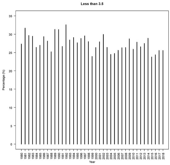
Figure 2.
Offshore wind speeds lower than 3.5 m/s.
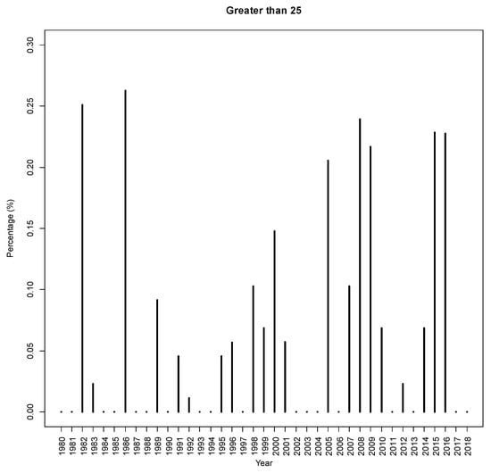
Figure 3.
Offshore wind speeds higher than 25 m/s.
Moreover, as displayed in Figure 4, 90% of the time, wind speeds are below 13 m/s. In other words, the full generation capacity for each turbine of 5.2 MW is realized only 10% of the time. These extreme wind volumes reflect the passage of typhoons over the wind farm.
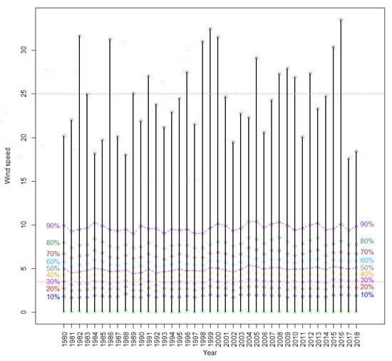
Figure 4.
Offshore percentile wind speeds.
As indicated by the monthly means in Figure 5, wind speeds are substantially higher in winter than in summer because the monthly mean speeds of the northeasterly along the Taiwan Strait increase rapidly with the onset of the winter monsoon. Figure 5 explains the significant impacts of the season on wind speed. In Taiwan, energy consumption peaks in summer as temperatures increase at the maximum. Because the wind speed is low during this season, Taiwan’s power needs cannot be met solely through offshore wind power.

Figure 5.
Monthly offshore wind speeds.
2.3. Offshore Wind Power Analysis
We calculate the rated power of 5.2 MW and examine the manufacturer-generated power curve to capture its relationship during the effective wind speeds from 3.5 to 25 m/s and thus forecast wind power output. These power outputs are gross estimates of AEP; because the turbine’s downtime and availability are not considered, the turbines can operate at their rated power year-round, maximizing the amount of power generated.
On the basis of the power curve, annual wind speed data (corresponding to the hub height) and time series AEP data at the wind farm are compiled (Figure 6). Details on the energy outputs are provided in Table 2.
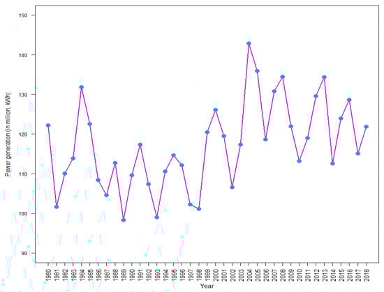
Figure 6.
Annual energy produced during the study period.
Table 2.
Annual energy production (MWh).
The wind data analysis indicates that wind speeds at the study site follow highly seasonal patterns and vary throughout the year. This explains why power outputs tend to be higher during the winter and lower during the summer. The estimated AEP can be expressed within a given confidence interval. The p values (e.g., P50 and P90) describe the probability that energy generation exceeds a certain percentage. Specifically, P50 denotes the annual average of power generation where the AEP is forecasted to be exceeded with a 50% probability over a year. P90 means that the AEP is forecasted to be exceeded with a 90% probability over a year.
Regarding the AEP calculations and considering the significant seasonal fluctuations in wind speeds, we further calculate the exceedance probabilities for estimated monthly energy production. Herein, the concept is the same as AEP, except that the p values represent monthly power output predictions. For example, P50 refers to the possibility that monthly power outputs are exceeded in 50% of the months. Accordingly, the P75 (P90) values represent the possibility that these outputs are exceeded in 75% (90%) of the months. Therefore, the quotient obtained from dividing P75 by P90, which is lower than P50, represents the simulation results of the long-term average. Figure 7 presents the P50, P75, and P90 records in the monthly power output simulations, determined according to the effective wind speeds.

Figure 7.
P50, P75, and P90 records of monthly offshore wind power produced.
3. Modeling and Forecasting Energy Production for Offshore Wind Farms
This section concerns the modeling and forecasting of wind power production for offshore wind farms. An accurate assessment of the long-term wind speed at hub height is necessary for predicting the power output of an offshore wind farm, which in turn enables developers, investors, and lenders to make relevant evaluations and allows insurers to estimate risks under an index insurance scheme.
Because fluctuations in energy output are mainly attributed to variations in wind speed, this variability must be predicted and managed to prevent balancing problems related to energy production. Taiwan’s offshore wind speeds are influenced by seasonal factors such as typhoons, which impede wind speed forecasts. However, as mentioned, energy production can be predicted through statistical analysis, as well as by examining the seasonal impacts on monthly power outputs.
Let {; t = 1, 2, ⋯, T} denote the monthly series of wind power outputs. We first consider the following linear regression models:
where Timet denotes a time trend or time dummy; Mit denotes the month dummy, with i = 1, 2, ⋯, 12; and denotes random fluctuation. We use data for the period from January 1980 to December 2017 (38 years or T = 456 months) for model identification and construction. Data for the 12 months of 2018 are applied for model validation. The left panel of Table 3 shows the results of ordinary least squares estimation for Model (3). All data analyses are conducted using R [33]. Because the estimate for the coefficient of Timet is positive and significant, we conclude that wind speeds slightly increase over the study period. The reason for this remains unclear; the world has become increasingly stormy over the past two decades. A report by National Geographic [34] indicates that wind speeds have increased by an average of approximately 5% over the preceding 20 years. Furthermore, according to new data from global satellites, the frequency of extreme strong winds caused by storms has increased by 10% over the same period.
Table 3.
Estimation results for Model (3) and Models (4) and (5).
On a monthly basis, this effect is clear and significant. The windiest period is between November and February because of the wintertime northeast monsoon. Despite the occasional occurrence of typhoons in summer and autumn, the winds remain fairly smooth from June to October. However, electricity shortages occasionally occur in Taiwan in the summer.
We employ the modeling strategies for time series analysis proposed by [35] and further discussed by [36] to model and decompose the various stochastic components underlying the data series on monthly wind power outputs. The following model serves as one of our optimal models:
where Ndayst indicates the number of days for month t. Here, the error term follows a first-order ARIMA model for each part of the autoregression and the moving average. This can be expressed as follows:
The right panel of Table 3 displays the estimation results for Models (4) and (5). The inclusion of Ndays yields negative estimates of yi. This is a reason for including the model results for comparison. Moreover, R2 increases slightly from 53.19% to 56.30%.
In Model (3) as well as in Models (4) and (5), a deterministic trend and deterministic seasonality are used, respectively, to model the presence of a linear trend and the effect of months on the data. To adjust for complex fluctuations, we consider the stochastic trend and stochastic seasonality by employing the multiplicative seasonal ARIMA model, denoted as ARIMA(p, d, q) × (P, D, Q)s. This model is detailed in chapter 9 of [35]. One of our optimal models for the monthly wind power output series is ARIMA(1, 1, 2) × (0, 1, 1)12, which can be expressed as follows:
where and B denote the backshift or lag operator, defined as Bkyt = yt−k. Table 4 presents the estimation results of Model (4). Although these estimations are lower than those of Models (4) and (5), Model (6) is more parsimonious because the Akaike information criterion and Bayesian information criterion are smaller than their counterparts for the other models.
Table 4.
Estimation results for Model (6).
Figure 8 and Figure 9 present the residual plots of Models (4) and (5) and of Model (6), respectively, along with their actual and fitted values. Because the trend and seasonality of the original data series are considered in the models, neither residual plot reveals a pattern. The residual diagnostics for both models follow the error assumptions of the models.
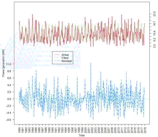
Figure 8.
Residual plot for Models (4) and (5).
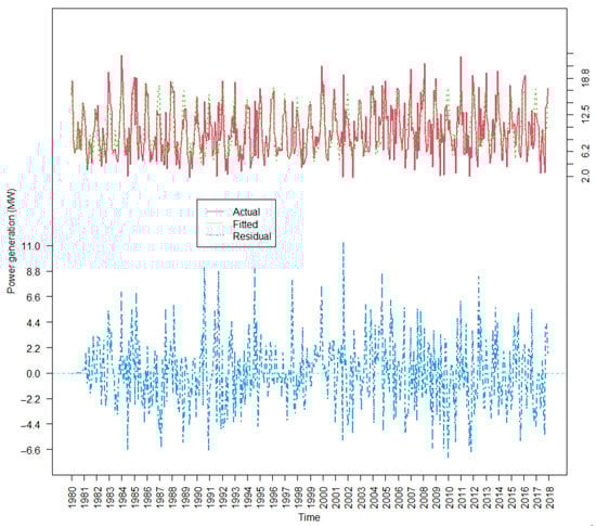
Figure 9.
Residual plot for Model (6).
Next, we apply the model estimates to produce a forecast for comparison with the model fit performance. To aid visual interpretation, Figure 10 and Figure 11 show part of the historical data (2014–2017) of wind power production and a 12-month extrapolation forecast for 2018 obtained by applying estimates from Models (4) and (5) and Model (6), respectively. The solid line with “◦” indicates the actual observation, whereas the dashed line with “•” denotes the fitted data from before December 2017 and the out-of-sample predicted data for 2018. The shaded area represents 95% interval extrapolation forecasts. For both models, all realizations are within the 95% forecast interval. Thus, the results appear reasonable overall.
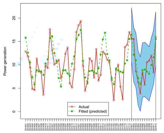
Figure 10.
Time plot of the fitted and predicted values of Models (4) and (5).
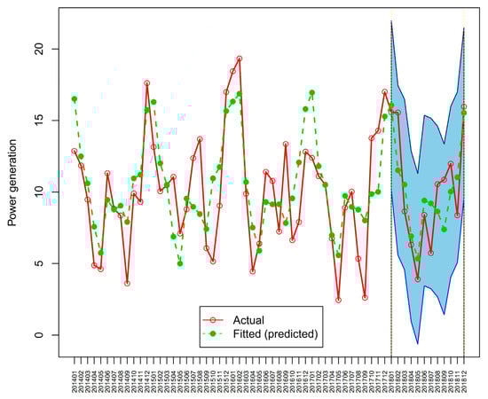
Figure 11.
Time plot of the fitted and predicted values of Model (6).
4. AEP Index Insurance
Wind speed risk differs from many types of risk covered under conventional property and liability insurance schemes for offshore wind farms. Index insurance has the potential to manage the production volatility risks incurred by offshore wind farms. Once wind speeds at a particular site are estimated, the value of generated energy can be assessed as the AEP index. This index insurance product can manage the impacts of risks from excessively high or low wind speeds on energy production and support project investments and financing decisions.
In general, index insurance involves some level of basis risk. The insurance contract must minimize such risk by using independently verifiable indexes as direct indexes that cannot be easily manipulated by either the insurer or the insured. As an independent index, wind speed data are objective and transparent; furthermore, they correlate strongly with wind power generation. Regarding the payout trigger, the AEP index is defined by the wind speed index and is used to calculate the payouts upon the completion of the insurance period. Thus, the insurance contract can be easily implemented using wind speed data. In turn, wind speed data can be used to estimate AEP and thereby determine a baseline against which the insured’s needs to establish the trigger index are considered. From the perspective of developers, investors, and lenders, such an insurance product might be attractive because it can stabilize the revenue gained from power generation.
Regarding AEP predictions, p values denote the long-term probability that the AEP is exceeded, as computed on the basis of historical wind speed data recorded at hub height at a given offshore wind farm. The power curve, which presents the electricity output of a turbine as a function of the wind speed and hub height, is generated and provided by the turbine manufacturer as per industry standards. Because the measured data are average hourly wind speeds, gross energy production per day is calculated by applying the power curve to the hourly average wind speed at hub height. The results are then integrated over one day, after which the net energy production per day is determined by adjusting for all system losses. The AEP index is derived by integrating the net daily energy production for all installed turbines at the wind farm over a 1-year insurance period.
System losses are loss factors applied to power generation at offshore wind farms. Most loss factor values are derived from industry standards. They are recorded either according to manufacturer-provided technical specifications or as indicated in the feasibility report of a given wind farm [37]. System losses, assumed to be constant throughout the 1-year insurance period, are estimates of a reduction in energy production. Thus, because of system losses, the net AEP of an offshore wind farm is less than the gross AEP. In the present insurance scheme, we define system efficiency as calculated from the aggregated influence of all system losses, including those from the wake effect, turbine availability, and electrical transmission efficiency. For example, suppose 6% of energy loss is ascribed to the wake effect (one component of the estimated power loss), and other sources account for 10–12% of energy loss. In that case, total system losses can approach 18%. Thus, the system efficiency ratio (SER) for the wind farm is 82%. Average power losses reported for the offshore wind farms Horns Rev, Lillgrund, and Nysted range from 10% to 25% of total power outputs [38,39]. Offshore wind projects have benefitted from the regulatory support of Taiwan’s government in providing higher purchase prices for power generation. The price of electricity generated by offshore wind farms is specified for a set period of 20 years under a FIT program as the applicable tariff for this index insurance product.
According to the AEP index, the insured will be compensated for any shortfall in energy production attributed to overly high or low wind speeds, irrespective of the occurrence of real loss and the extent of said loss. With reference to area yield crop insurance [40,41], the predefined AEP is referred to as the index trigger. Payouts are structured in a proportional schedule as follows:
Financial modeling requires a comprehensive understanding of all project assumptions. Furthermore, a sensitivity analysis must be conducted to define a financial base case. Therefore, in the planning and financing stages of a wind farm project, wind resources must be evaluated to quantify all financing-related risks [42].
Through the aforementioned methods, developers and lenders can transfer the financial risk of wind volatility to insurers to minimize the effect of revenue losses. Using AEP estimates to decide a trigger level and p values for an insurance contract are considered reliable. Moreover, it can demonstrate that the uncertainty is at a level acceptable to most stakeholders. On the basis of the theoretical framework of AEP analysis, P90 is widely adopted by lenders and investors as a foundation for financial decision-making [43]. Thus, as shown in Figure 12, we respectively apply P90 and P99 to the Changhua Demonstration Offshore Wind Farm as the index trigger and the deductible. Over the analytical period, the realized index does not reach P90 on five occasions: in 1981, 1989, 1993, 1997, and 1998.
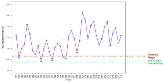
Figure 12.
Payouts based on P90 for annual energy production.
In index insurance, reducing basis risk is critical because the index is a predictor of energy production losses associated with payouts. Furthermore, the independence of the data provider is essential, and the data provided must be mutually agreed upon by the insurer and the insured. After the 1-year insurance period, the wind farm can use actual system loss data to benchmark the actual SER and thereby reduce the basis risk ascribable to system losses.
In the future, once actual AEP data become available, the present index insurance scheme can employ the actual AEP of the insured as another trigger from which to adjust scheme design in order to further reduce basis risks.
5. Pure Premium AEP Index Insurance Rates
To reduce the basis risk, seasonal impacts to power generation are taken into account at monthly time scales as inputs in the insurance pricing strategies. A historical wind speed database is required for pricing the index insurance scheme to estimate energy production and apply statistical methods for fitting distribution functions to the collected data. Exceedance probability constitutes a statistical measure of whether the probability for a particular value will be reached or exceeded. For example, a 50% exceedance probability (P50) is equal to the mean value of a population’s probability density function, where 50% of the probability density is above and below the mean, respectively. P75 indicates that the probability that the P75 value will not be attained is 25%.
With reference to Section 3, Figure 13 and Figure 14 display the autocorrelation function (ACF) and partial autocorrelation function plots of the residuals based on Model (6). Neither indicates serial correlation.
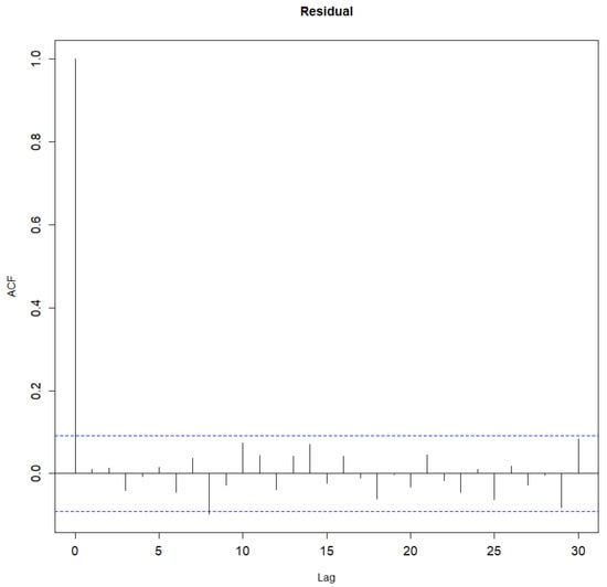
Figure 13.
The autocorrelation function plots of the residuals based on Model (6).
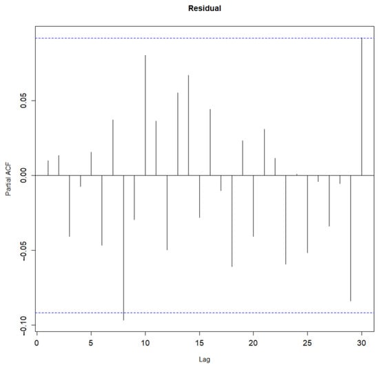
Figure 14.
The partial autocorrelation function plots of the residuals based on Model (6).
Figure 15 and Figure 16 present the histogram and normal probability plot of the residuals based on Model (6), respectively. Again, the residuals appear relatively symmetrical and, except for a few points with large positive deviations, follow a normal distribution.
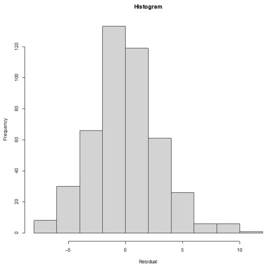
Figure 15.
The histogram plot of the residuals based on Model (6).
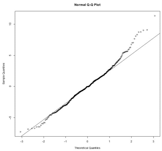
Figure 16.
The normal probability plot of the residuals based on Model (6).
Therefore, we can conclude that Model (6) residuals are independent and identically distributed with a normal distribution. Assuming a normal distribution for those uncertainties in monthly energy production facilitates the determination of the pure premium through the computation of the exceedance probabilities for the corresponding p values within the mean and standard deviation. P50 is the mean value of the distribution; the standard deviation herein is a measure of the spread of p values around P50. Thus, we can estimate the uncertainty to be defined as the standard deviation about the mean for the remaining p values.
Across all timescales, wind speeds exert impacts on the technical performance of offshore wind farms. Specifically, significantly more power is generated, and wind speeds are substantially stronger during the winter months than during the summer months. AEP is the main consideration for developers, investors, and lenders in offshore wind projects. The financing community views offshore wind power as stable on an annual basis. However, this is only true if they assess AEPs for complete calendar years. In insurance pricing models, the volatility of wind power must be acknowledged through the assessment and consideration of seasonal fluctuations in power outputs. Our pricing approach is to divide the AEP time series into monthly sequences, where we examine disjointed sequences for each year from 1980 to 2018 rather than a single time series. Instead of using the AEP time series, monthly wind speed variability is considered for estimating energy outputs. Each year’s monthly energy production time series are concatenated, as shown in Figure 17.
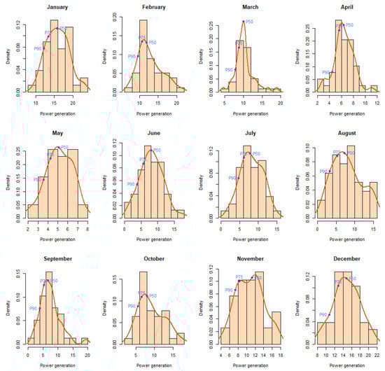
Figure 17.
P50, P75, and P90 records of monthly energy production.
Through the further application of the p values of monthly energy production (MEP), we propose a conventional approach for calculating the exceedance probabilities for a given MEP of the Changhua Demonstration Offshore Wind Farm as follows:
Considering the expected value as well as the P50 and corresponding standard deviation of MEP, the exceedance probabilities for certain energy production levels associated with monthly forecasts can be derived from the MEP distribution curve. In Equation (8), a is the p value of MEP, x is the corresponding forecast value of MEP, b is the retention (i.e., b = P99), and the difference of a and b is the limit of liability. Once each monthly premium is derived, all monthly premiums can be aggregated to obtain the annual pure premium. The MEP estimates with 90% and 75% exceedance are used as defined inputs in our pricing analysis under 90% and 75% confidence levels, respectively. Table 5 presents the approximate pure premium of the index insurance scheme. The estimated pure premium rate for the wind farm is 5.96% for P90 and 11.55% for P75.
Table 5.
Estimated pure premium rates of index insurance for the selected offshore wind farm.
6. Discussions
Research on wind power application worldwide has been developed to estimate offshore wind source potential as the critical step for project feasibility analysis [44,45,46,47]. Most research focuses on analyzing offshore wind data probability distribution and evaluating offshore wind energy resources over a large area in Taiwan. For example, Lee [48] studied the Fuzzy Analytic Hierarchy Process (Fuzzy AHP) application combined with criteria analysis for selecting appropriate sites for developing offshore wind energy in Taiwan. Chang et al. [49] used wind speed data observed by buoys and tidal stations at various locations for months to forecast wind speeds at different heights on the west coast of Taiwan for offshore areas in Hsinchu, Miaoli, Taichung, Changhua, Yunlin, Chiayi, and Tainan. Fang [50] used the most common software suite, the Wind Analysis and Application Program (WAsP) [51] for wind resource assessment for the offshore areas of Taiwan’s west coast for the relative financial planning of offshore wind projects. The average wind speeds of the areas along the west coast of Taiwan are about 9.5 m/s, and the power density is about 1000 w/. All studies indicate that the offshore area of Taiwan’s west coast has excellent wind energy potential and is worth developing offshore wind farms. Wind speeds vary based on location; wind energy assessment over large areas can reference offshore wind energy potential. The AEP evaluation of an offshore wind farm needs a site-specific analysis. However, very little research has been conducted for a site-specific offshore wind farm in Taiwan.
A recent project was conducted by Cheng et al. [52] for the first offshore wind farm in Taiwan; the Formosa 1 offshore wind farm was completed in October 2019, which has a total capacity of 128 MW and is located about 6 km off the coast of Miaoli in northwestern Taiwan. This study used the met mast wind speed data for one year of the farm, from May 2017 to April 2018, to investigate the wind speed characteristics of the offshore wind farm, modeling the probability distribution and characterizing the seasonal variation of the at-site wind speed. The met mast is installed within the farm site, which carries measuring instruments to measure wind speed and can provide data at frequent intervals, such as every ten minutes. Those data can provide the project developer to determine whether the site is economically viable for an offshore wind farm and select offshore wind turbines optimized for local wind speed distribution. This study used statistical approaches and the one-year wind speed data to analyze the annual mean and standard deviation and probability density function of wind speed. However, the power curve of the selected wind turbine was difficult to obtain, so the study used a reference wind turbine to calculate annual energy output instead. Without yearly time series data of wind speed, the AEP is calculated for one year only.
Our article also uses statistical approaches to analyze offshore wind energy for a specific offshore wind farm compared to the above study. The exceedance probabilities of the AEP are critical for lenders’ underwriting for renewable energy projects. The AEPs are calculated by 39 years of hourly wind speed data at hub height based on the selected wind turbine. The local wind speed profile between the Formosa 1 and the Changhua demonstration offshore wind farm is similar from the study results. The two farm sites are located off the coast of western Taiwan, about 6–7 km to shore, and the seasonal effect and the monsoon cause the principal fluctuation of monthly mean wind speed. Therefore, to assess potential offshore wind energy in Taiwan, the AEPs should be calculated with the MEPs at offshore wind farm locations to reflect the monthly variation on wind energy generation.
As we mentioned in the introduction to this article, many studies focus on applying index insurance for agriculture; however, there are comparatively very few in the renewable energy sector, especially for wind energy. Han et al. [53] proposed a similar weather index insurance design for wind energy to avoid economic losses caused by weather risks. According to the findings of the study, the wind-speed power generation index is generated by the theoretical on-grid power based on the actual wind speed of the farm site and specified the accounting rules and impact factors. The theoretical on-grid power has a conversion rate to the actual grid power determined by consultation between the insurer and the insured. The trigger point is assumed that 90% of the theoretical on-grid power of the insured wind farm. The weather index insurance pricing used the classical combustion analysis method; it assumes that the probability distribution of future loss is consistent with that of historical experience and takes the expected value of historical data compensation value for pure premium calculation. This study took 2017 data provided by an onshore wind farm in Xinjiang, China, to illustrate the index insurance application and found seven months were triggered due to low-wind resources in the same year.
In our paper, the AEP index is developed along with a large set of available weather and satellite data provided by an independent third party that accounts for the exceedance probabilities in wind energy output for the insured wind farm to be more scientific, with less human influence. The reliance on manual data collection is easy to associate with a higher error risk. Data used from an independent third party for index insurance can reduce administration/data collection costs and opportunities for manipulation and minimize moral hazards and adverse selection problems. Our pricing model uses the monthly forecasts generated by our forecasting models in Section 3. By applying the p values of MEP, we propose a conventional approach for calculating the exceedance probabilities for the given MEP. Considering the expected value and the P50, and the corresponding standard deviation of MEP, the exceedance probabilities for certain energy production levels associated with monthly forecasts can be derived from the MEP distribution curve. Once each monthly premium is derived, all monthly premiums can be aggregated to obtain the annual pure premium.
Insurance is one of the methods for mitigating risks. Our study has policy implications for promoting risk management of renewable energy due to production volatilities for offshore wind development in Taiwan. The study provides evidence that index insurance can cover offshore wind farms for the loss of energy production due to lack of wind to encourage investments in renewable energy. Although the results of our study indicate that the index insurance can reduce energy production volatilities for offshore wind projects, it remains to be seen whether this product could be commercially feasible or just an innovative design. Most lenders have limited experience and capacity to underwrite offshore wind projects in Taiwan. However, higher energy production certainty for an offshore wind project means a lower risk exposure to the lender. Future research will analyze whether positive experiences with this insurance product can stimulate future demand by cost-benefit calculations for offshore wind project stakeholders; to see the reduction in the cost of financing is sufficient to make the product commercially viable. If not, subsidizing the insurance or reinsurance premium may be a consideration for Taiwan government interventions; the long-term benefits of renewable energy to the public and the environment protection may exceed the costs.
7. Conclusions
In this study, we designed an insurance policy on the basis of wind speed indexes over a specified period by using wind data collected from the Changhua Demonstration Offshore Wind Farm.
A key challenge in the preconstruction phase of offshore wind projects is providing sufficient evidence to support the proposed benefits such that lenders and investors consider them in project financing. Our index insurance product provides a useful framework for addressing financial risk in power generation. Developers and investors can evaluate their project plans so that lenders can minimize risks by returning loans and interest at appropriate scales. The present findings can provide a solution for mitigating the volume volatility associated with wind resources and improve the financial conditions under which offshore wind projects are developed. In contrast to conventional insurance products, our insurance scheme can serve as a financial package for evaluating new offshore wind projects through the consideration of actual investments. Because claims in index insurance policies are settled based on a measurable objective index instead of the insured’s actual losses, both the insurer and the insured must be confident that AEP calculations in trigger payouts are accurate and transparent.
Although index insurance products have several advantages over conventional insurance products in terms of reducing the risk of adverse selection and preventing moral hazards, they also have a serious limitation: introducing basis risk. As offshore wind turbines grow taller, building representative datasets means having to extrapolate original data to hub height, increasing the uncertainty in the measured power.
Notably, our index insurance scheme can be used as a foundation for developing broader risk management strategies because it removes one of the major constraints in the renewable energy industry. Regarding commercial applications, the development of our index insurance product requires an economical premium of reasonable size. Once the insurance contract is established, necessary support can be obtained from reinsurance markets to make the scheme commercially viable. Given the considerable capacity of the future offshore wind projects in Taiwan, this index insurance product development is promising. In the future, it can be applied in other countries. To mitigate various potential weather-related risks, we intend to apply this similar approach for other renewable resources. We hope that projects in the renewable energy industry gradually see more financial support based on well-designed index insurance schemes.
Author Contributions
Conceptualization, S.-C.L.; methodology, S.-C.L., T.-C.C. and S.-C.C.; software, T.-C.C. and S.-C.L.; validation, S.-C.L. and T.-C.C.; formal analysis, T.-C.C.; investigation, S.-C.L.; resources, S.-C.L.; data curation, T.-C.C.; writing—original draft preparation, S.-C.L.; writing—review and editing, S.-C.L. and T.-C.C.; visualization, T.-C.C.; supervision, S.-C.C.; project administration, S.-C.L. All authors have read and agreed to the published version of the manuscript.
Funding
This research received no external funding.
Institutional Review Board Statement
This study did not require ethical approval.
Informed Consent Statement
Not applicable.
Data Availability Statement
Publicly available datasets were analyzed in this study. This data can be found here: https://disc.gsfc.nasa.gov/datasets/M2T1NXSLV_V5.12.4/summary (accessed on 7 August 2021).
Conflicts of Interest
The authors declare no conflict of interest.
References
- The Paris Agreement. Available online: https://www.un.org/en/climatechange/paris-agreement (accessed on 2 July 2021).
- 4C Offshore. Global Offshore Wind Speeds Ranking. Available online: http://www.4coffshore.com/windfarms/windspeeds.aspx (accessed on 2 July 2021).
- Chantarat, S.; Mude, A.G.; Barrett, C.B.; Carter, M.M. Designing Index-based Livestock Insurance for Managing Asset Risk in Northern Kenya. J. Risk Insur. 2013, 80, 205–237. [Google Scholar] [CrossRef]
- Carter, M.; Janvry, A.D.; Sadoulet, E.; Sarris, A. Index-Based Weather Insurance for Developing Country: A Review of Evidence and A Set of Propositions for Up-Scaling; Working Paper; Fondation Pour les études et Recherches sur le Développement International: Paris, France, 2014. [Google Scholar]
- SDGs. Available online: https://sdgs.un.org/goals (accessed on 2 July 2021).
- Allen, L.; Jagtiani, J. The Risk Effects of Combining Banking, Securities, and Insurance Activities. J. Econ. Bus. 2000, 52, 485–497. [Google Scholar] [CrossRef]
- Chantarat, S.; Barrett, C.B.; Mude, A.G.; Turvey, C.G. Using Weather Index Insurance to Improve Drought Response for Famine Prevention. Am. J. Agric. Econ. 2007, 89, 1262–1268. [Google Scholar] [CrossRef]
- Skees, J.R.; Gober, S.; Varangis, P.; Lester, R.; Kalavakonda, V. Developing Rainfall-Based Index Insurance in Morocco; Working Paper; The World Bank: Washington, DC, USA, 2001. [Google Scholar]
- Hess, U.; Richter, K.; Stoppa, A. Weather Risk Management for Agriculture and Agri-business in Developing Countries. In Climate Risk and the Weather Market, Financial Risk Management with Weather Hedges; Risk Books: London, UK, 2002. [Google Scholar]
- Barnett, B.J.; Mahul, O. Weather Insurance Index for Agriculture and Rural Areas in Lower Income Countries. Am. J. Agric. Econ. 2007, 89, 1241–1247. [Google Scholar] [CrossRef]
- Osgood, D.; McLaurin, M.; Carriquiry, M.; Mishra, A.; Fiondella, F.; Hansen, J.; Peterson, N.; Ward, N. Final Report to the Commodity Risk Management Group ARD. In Designing Weather Insurance Contracts for Farmers in Malawi, Tanzania and Kenya; The World Bank: Washington, DC, USA, 2007. [Google Scholar]
- Skees, J.R. Innovation in Index Insurance for the Poor in Lower Income Countries. Agric. Resour. Econ. Rev. 2008, 37, 1–15. [Google Scholar] [CrossRef]
- Iturrioz, R. Agricultural Insurance; Primer Series on Insurance Issue; The World Bank: Washington, DC, USA, 2009. [Google Scholar]
- Manuamorn, O.P. Agriculture and Rural Development Discussion Paper. In Scaling Up Microinsurance: The Case of Weather Insurance for Smallholders in India; The World Bank: Washington, DC, USA, 2005. [Google Scholar]
- Alderman, H.; Haque, T. Insurance Against Covariate Shocks-the Role of Index Based Insurance in Social Protection in Lower Income Countries of Africa; Working Paper; The World Bank: Washington, DC, USA, 2007. [Google Scholar]
- Carter, M.; Janvry, A.D.; Sadoulet, E.; Sarris, A. Index Insurance for Developing Country Agriculture: A Reassessment. Annu. Rev. Resour. Econ. 2017, 9, 421–438. [Google Scholar] [CrossRef]
- Vedenov, D.V.; Barnett, B.J. Efficiency of Weather Derivatives as Primary Corp Insurance Instruments. J. Agric. Resour. Econ. 2004, 29, 387–403. [Google Scholar]
- Breustedt, G.; Bokusheva, R.; Heidelbach, O. Evaluating the Potential of Index Insurance Schemes to Reduce Crop Yield Risk in an Arid Region. J. Agric. Econ. 2008, 59, 312–328. [Google Scholar] [CrossRef]
- de Janvry, A.; Sadoulet, E. From Indemnity, Index-Based, and Group Weather Insurance Contracts; Policy Brief Note 25; Fondation Pour les études et Recherches sur le Développement International: Paris, France, 2011. [Google Scholar]
- Hazel, P.; Anderson, J.; Balzer, N.; Clemmensen, A.H.; Hess, L.I.; Rispoli, F. The Potential for Scale and Sustainability in Weather Index Insurance for Agriculture and Rural Livelihood; International Fund for Agricultural Development and World Food Programme: New York, NY, USA, 2010. [Google Scholar]
- Pelka, N.; Musshoff, O. Hedging Effectiveness of Weather Derivatives in Erable Farming—Is There a Need for Mixed Indices? Agric. Financ. Rev. 2013, 73, 358–372. [Google Scholar] [CrossRef]
- Calif, R.; Schmitt, F. Modeling of Atmospheric Wind Speed Sequence Using a Lognormal Continuous Stochastic Equation. J. Wind Eng. Ind. Aerodyn. 2012, 109, 1–8. [Google Scholar] [CrossRef]
- Jung, C.; Schindler, D. On the Inter-Annual Variability of Wind Energy Generation—A Case Study from Germany. Appl. Energy 2018, 230, 845–854. [Google Scholar] [CrossRef]
- Chang, W.Y. A Literature Review of Wind Forecasting Methods. J. Power Energy Eng. 2014, 2, 161–168. [Google Scholar] [CrossRef]
- Wang, X.; Guo, P.; Huang, X. A Review of Wind Power Forecasting Models. Energy Procedia 2011, 2, 770–778. [Google Scholar] [CrossRef]
- Pinson, P. Wind Energy: Forecasting Challenges for its Operational Management. Stat. Sci. 2013, 28, 564–585. [Google Scholar] [CrossRef]
- Tabas, D.; Fang, J.; Porté-Agel, F. Wind Energy Prediction in Highly Complex Terrain by Computational Fluid Dynamics. Energies 2019, 7, 1311. [Google Scholar] [CrossRef]
- Okumus, I.; Dinler, A. Current Status of Wind Energy Forecasting and a Hybrid Method for Hourly Predictions. Energy Convers. Manag. 2016, 123, 362–371. [Google Scholar] [CrossRef]
- Barnett, B.J.; Barrett, C.B.; Skees, J.R. Poverty Traps and Index-Based Risk Transfer Products. World Dev. 2008, 36, 1766–1785. [Google Scholar] [CrossRef]
- Pinker, R.T.; Frouin, R.; Li, Z. A Review of Satellite Methods to Derive Surface Shortwave Irradiance. Remote Sens. Environ. 1995, 51, 108–124. [Google Scholar] [CrossRef]
- De Wit, A.J.; Van Diepen, C.A. Crop Growth Modelling and Crop Yield Forecasting Using Satellite-derived Meteorological Inputs. Int. J. Appl. Earth Obs. Geoinf. 2008, 10, 414–425. [Google Scholar] [CrossRef]
- Bansal, R.C.; Bati, T.S.; Kothari, D.P. On Some of the Design Aspects of Wind Energy Conversion Systems. Energy Convers. Manag. 2002, 43, 2175–2187. [Google Scholar] [CrossRef]
- The R Project for Statistical Computing. Available online: https://www.r-project.org (accessed on 3 March 2021).
- Inman, M. Earth Getting Mysteriously Windier. National Geographic. 2011. Available online: https://www.nationalgeographic.com/news/2011/3/110328-earth-storms-winds-global-warming-science-environment/ (accessed on 2 July 2021).
- Box, G.E.P.; Jenkins, G.M.; Reinsel, G.C. Time Series Analysis: Forecasting and Control, 3rd ed.; Prentice-Hall: Englewood Cliffs, NJ, USA, 1994. [Google Scholar]
- Diebold, F.X. Elements of Forecasting, 4th ed; Cincinnati: South-Western, OH, USA, 2007. [Google Scholar]
- Ortega, C.; Younes, A.; Severy, M.; Chamberlin, C.; Jacobson, A. Resource and Load Compatibility Assessment of Wind Energy Offshore of Humboldt County, California. Energies 2020, 13, 5707. [Google Scholar] [CrossRef]
- Barthelmie, R.J.; Pryor, S.C.; Frandsen, S.T.; Hansen, K.S.; Schepers, J.G.; Rados, K.; Schlez, W.; Neubert, A.; Jensen, L.E.; Neckelmann, S. Quantifying the Impact of Wind Turbine Wakes on Power Output at Offshore Wind Farms. J. Atmos. Ocean. Technol. 2010, 27, 1302–1317. [Google Scholar] [CrossRef]
- Wu, Y.T.; Porte-Agél, F. Modeling Turbine Wakes and Power Losses within A Wind Farm Using LES: An Application to the Horns Rev Offshore Wind Farm. Renew. Energy 2015, 75, 945–955. [Google Scholar] [CrossRef]
- Miranda, M.J. Area-yield Crop Insurance Reconsidered. Am. J. Agric. Econ. 1991, 73, 233–242. [Google Scholar] [CrossRef]
- Skees, J.R.; Black, J.R.; Barnett, B.J. Designing and Rating an Area-yield Crop Insurance Contract. Am. J. Agric. Econ. 1997, 79, 430–438. [Google Scholar] [CrossRef]
- Judgea, F.; McAuliffea, F.D.; Sperstadb, I.B.; Chestera, R.; Flannerya, B.; Lyncha, K.; Murphy, J. A Lifecycle Financial Analysis Model for Offshore Wind Farms. Renew. Sustain. Energy Rev. 2019, 103, 370–383. [Google Scholar] [CrossRef]
- Mora, E.B.; Spelling, J.; van der Weijde, A.H.; Pavageau, E. The Effects of Mean Wind Speed Uncertainty on Project Finance Debt Sizing for Offshore Wind Farms. Appl. Energy 2019, 252, 113419. [Google Scholar] [CrossRef]
- Schwartz, M.; Heimiller, D.; Haymes, S.; Musial, W. Assessment of Offshore Wind Energy Resources for the United States; National Renewable Energy Laboratory: Golden, CO, USA, 2010. [Google Scholar]
- Lee, M.E.; Kim, G.; Jeong, S.-T.; Ko, D.H.; Kang, K.S. Assessment of Offshore Wind Energy at Younggwang in Korea. Renew. Sustain. Energy Rev. 2013, 21, 131–141. [Google Scholar] [CrossRef]
- Yu, J.; Fu, Y.; Yu, F.; Wu, S.; Wu, Y.; You, M.; Guo, S.; Li, M. Assessment of Offshore Wind Characteristics and Wind Energy Potential in Bohai Bay, China. Energies 2019, 12, 2879. [Google Scholar] [CrossRef]
- Ranthodsang, M.; Waewsak, J.; Kongruang, C.; Gagnon, Y. Offshore Wind Power Assessment on the Western Coast of Thailand. Energy Rep. 2020, 6, 1135–1146. [Google Scholar] [CrossRef]
- Lee, T.L. Assessment of the Potential of Offshore Wind Energy in Taiwan Using Fuzzy Analytic Hierarchy Process. Open Civ. Eng. J. 2010, 4, 96–104. [Google Scholar] [CrossRef][Green Version]
- Chang, P.C.; Yang, R.Y.; Lai, C.M. Potential of Offshore Wind Energy and Extreme Wind Speed Forecasting on the West Coast of Taiwan. Energies 2015, 8, 1685–1700. [Google Scholar] [CrossRef]
- Fang, H.F. Wind Energy Potential Assessment for the Offshore Areas of Taiwan West Coast and Penghu Archipelago. Renew. Energy 2014, 67, 237–241. [Google Scholar] [CrossRef]
- Langea, B.; Højstrup, J. Evaluation of the Wind-resource Estimation Program WAsP for Offshore Applications. J. Wind Eng. Ind. Aerodyn. 2001, 89, 271–291. [Google Scholar] [CrossRef]
- Cheng, K.S.; Ho, C.Y.; Teng, J.H. Wind Characteristics in the Taiwan Strait: A Case Study of the First Offshore Wind Farm in Taiwan. Energies 2020, 13, 6492. [Google Scholar] [CrossRef]
- Han, X.; Zhang, G.; Xie, Y.; Yin, J.; Zhou, H.; Yang, Y.; Li, J.; Bai, W. Weather Index Insurance for Wind Energy. Glob. Energy Interconnect. 2019, 2, 541–548. [Google Scholar] [CrossRef]


Publisher’s Note: MDPI stays neutral with regard to jurisdictional claims in published maps and institutional affiliations. |
© 2021 by the authors. Licensee MDPI, Basel, Switzerland. This article is an open access article distributed under the terms and conditions of the Creative Commons Attribution (CC BY) license (https://creativecommons.org/licenses/by/4.0/).