Article

Evaluation of Profiles of Standard Deviation of Vertical Wind in the Urban Area of Rome: Performances of Monin–Obukhov Similarity Theory Using Different Scaling Variables

by
Armando Pelliccioni
1,*,
Livia Grandoni
1,2 and
Annalisa Di Bernardino
3
1
Compensation Authority (INAIL), Monte Porzio Catone, 00078 Rome, Italy
2
Department of Civil, Constructional and Environmental Engineering, Sapienza University, 00185 Rome, Italy
3
Physics Department, Sapienza University, 00185 Rome, Italy
*
Author to whom correspondence should be addressed.
Sustainability 2021, 13(15), 8426; https://doi.org/10.3390/su13158426
Submission received: 4 June 2021 / Revised: 13 July 2021 / Accepted: 23 July 2021 / Published: 28 July 2021

Abstract

:
The parametrizations of meteorological variables provided by the Monin–Obukhov similarity theory (MOST) is of major importance for pollutant dispersion assessment. However, the complex flow pattern that characterizes the urban areas limits the applicability of the MOST. In this work, the performance of different existing parametrizations of the standard deviation of vertical wind velocity were tested in the city of Rome. Results were compared with experimental data acquired by a sonic detection and ranging (SODAR) and a sonic anemometer. Different scaling variables estimated from the anemometer data by considering two coordinate systems—one aligned with the geodetic reference frame and the other following the flow streamlines—were used to evaluate the effects of flow distortion due to the presence of buildings. Results suggest that the MOST parametrizations perform better if the scaling variables obtained using the coordinate system following the flow streamlines are used. This estimation of the scaling variables would make it possible to overcome the difficulties in conducting measurements of turbulent fluxes, either at different altitudes or even in the constant flux layer.

1. Introduction

In atmospheric pollution modelling, knowledge of the meteorological variables is essential, as they govern transport and dispersion of the pollutants [1]. Among them, the most important variables are wind speed and direction, height of the mixing layer, and parameters linked with atmospheric turbulence. The latter plays a fundamental role in dispersive phenomena since it is effective at causing mixing, particularly in the atmospheric boundary layer (ABL, e.g., [2]).
Application of the governing equations of fluid mechanics describes and forecasts the dynamics and thermodynamics of the gases of the ABL. Unfortunately, the set of equations is so complex that no analytical solution is known, particularly in the case of turbulent flows. Similarity theory provides a way to organize and group the variables of interest and makes available a series of analytical expressions for their parameterization [3]. In the framework of ABL flows, the Monin–Obukhov similarity theory (MOST; [4]) has given rise to a profusion of considerable efforts in the search for general laws suitable for various atmospheric stability conditions [5]. The MOST states that the vertical profiles of some meteorological variables, such as wind velocity, air temperature, and turbulent fluxes, can be obtained by algebraic relationships dependent on the height and on the scaling variables. In principle, the MOST can be applied for steady and horizontally homogeneous conditions, when the wind is not calm, and the terrain is substantially devoid of orography or obstacles [2].
In the case of urban areas, the characteristics of the urban texture induce changes to the ABL, with consequent modifications of the dynamic, thermal, and water regimes compared to the surrounding rural areas [6,7,8,9,10,11,12]. The processes that cause such variations can be attributed mainly to alterations in the radiative energy budget of the local earth–atmosphere system, and aerodynamic phenomena such as wind channeling, recirculation, stagnation, and turbulence (Figure 1). In principle, the lower part of the ABL, also known as the surface layer (SL), is eroded from below by the urban canopy layer (UCL), i.e., the region that extends from the ground up to the mean building height (hb). Above the UCL, a roughness sublayer (RSL) forms, where the airflow is three-dimensional, non-homogenous, and still influenced by vegetation, buildings, and other roughness elements that constitute the urban canopy [13]. The RSL top is generally assumed to be 2–5 hb. Above the RSL, a constant flux layer (CFL) generally exists, where the turbulent fluxes of heat, momentum, and humidity can be considered nearly constant [14].
Despite the considerable efforts made in the last decades, there are still many open problems when applying MOST in an urban environment. For example, the expression for the vertical profile of the mean wind velocity [15,16]:
u ¯ ( z ) = ( u *   k ) [ ln ( z d 0 z 0 ) ψ m ( z L ) ]
could in principle be used only in the CFL. Here, the bar indicates the time average, z is the altitude, k = 0.4 is the von Karman constant, u * = τ 0 / ρ is the friction velocity, z 0 is the aerodynamic roughness length, d 0 is the displacement height, L is the Obukhov length, τ 0 is the stress at the surface, and ρ is the air density. z 0 and d 0 are generally estimated using the morphometric or the anemometric methods (e.g., [17]). ψ m is the similarity universal function, which depends on the atmospheric stability. It is equal to zero in neutral conditions ( ψ (0) = 0), i.e., when L tends to infinity. The Obukhov length represents the height above the ground at which the production/consumption of turbulent kinetic energy (TKE) due to buoyancy equals the TKE production due to shear [2]:
L = u * 3 T v ¯ ρ C p kgH s
and can be considered as a spatial scale of the flow in addition to z 0 in non-neutral conditions. Here, T v is the potential temperature, g the acceleration due to the gravity,   C p the specific heat at constant pressure, and H s the sensible heat flux, viz.:
H s = ρ C p w T v ¯
where   w     T v ¯ is the vertical component of the kinematic heat flux ( w is the fluctuation around the mean of the vertical wind velocity component and T v is the fluctuating virtual temperature).
The friction velocity, which represents the velocity scale for the CFL, is calculated from the (turbulent) vertical flux of momentum, viz.:
u * = [ ( u w ¯ ) 2 + ( v w ¯ ) 2 ] 1 4
where u and v are the zonal (positive towards east) and meridional (positive towards north) velocity components, respectively.
In addition to the mean velocity, MOST provides useful laws for the vertical profiles of the velocity variances and TKE, a parameter involved in dispersion models.
The greatest difficulty in applying the MOST lies in the availability of the turbulent fluxes of heat and momentum, by which the scaling variables ( u * and L) are determined. The MOST states that u * and L are referred to the CFL, whose identification, in the case of urban canopies, is not straightforward [18]. Indeed, meteorological data are routinely acquired by anemometers/thermometers installed in urban canyons or on rooftops, which are not representative of the CFL (e.g., [19,20]). Many studies have shown how the turbulent fluxes measured on terraces are affected by local airflow linked to the presence of the buildings, which substantially changes both the average velocity and the turbulent fluxes because of local disturbances [21,22,23]. In the case of regular arrays of cubic buildings (an ideal condition), the airflow above the rooftop changes remarkably in space and the measured data are influenced considerably by local flow distortion (see e.g., [24,25]). In most cases, the meteorological instruments are mounted on masts 2–5 m high, on the roof, where flow distortion is large and turbulence intensity can vary even of a factor of two with the wind direction only due to local flow distortion (e.g., [26]). This is a long-standing problem that makes the application of the MOST in urban environments rather problematic.
The present work started from the above considerations and aimed to analyze local flow distortion and its effects on u * and L calculated from wind data collected by a sonic anemometer installed on a 3.5 m mast located on a building rooftop. Two different coordinate systems were considered for the computation of friction velocity—sensible heat flux and Obukhov length. The first, hereinafter “normal” (nrm), coordinate system is aligned with the geodetic reference frame, while the second, hereinafter “tilted” (tilt), follows the flow streamlines and allows for consideration of flow distortion due to the presence of obstacles (e.g., buildings).
The meteorological dataset used for the analysis was acquired in Rome during the 2016–2018 field campaign of the VIEPI project (Integrated Evaluation of Indoor Particulate Exposure; [27]), which aimed to investigate the role played by micrometeorology and indoor airflow characteristics in determining indoor particulate matter concentration.
The aim of the present paper was twofold: (i) to evaluate the applicability of existing MOST formulations for vertical velocity standard deviation to the RSL above Rome and (ii) to assess whether the scaling variables considered in this work are reasonable. Different options for the scaling variables were tested. Particular attention was given to u * and L calculated just above a building based on the two coordinate systems mentioned above.
The paper is organized as follows. In Section 2, the MOST formulations chosen for comparison with our real-scale experimental data are shown. Additionally, our measuring site is described. Section 2 also shows the data processing (i). to obtain the different tested scaling variables and (ii). to compare our data to the existing MOST formulations. In Section 3, the main results are presented. Specifically, the u * and L obtained from the anemometer data in the two coordinate systems are shown and were compared, along with the u * estimated by the ground-based remote sensing sonic detection and ranging (SODAR). Finally, the existing MOST parameterizations for the standard deviation of vertical wind velocity were compared with the experimental data. In particular, the effect of the tilted coordinate system on the turbulent fluxes was assessed to evaluate the applicability of the different MOST parameterizations for our case study.

2. Materials and Methods

2.1. Parametrization of the Standard Deviation of Vertical Velocity

Several authors have tackled the application of MOST in cities and found formulations suitable both for urban areas and complex terrain (see Table 1). In the present work, the MOST parameterization for standard deviation of vertical wind velocity ( σ w ) proposed in the seven studies listed in Table 1 have been compared with those obtained by measurements by SODAR and sonic anemometer placed above the terrace of the Physical Department of Sapienza University of Rome (see [27] for details). All considered studies were based on the functional equation (see, e.g., [28]):
σ w u * = a   ( 1 + b   z L ) p
which relates σ w / u * to z / L and were valid irrespective of the stability condition. The parameters a, b, and p changed with the case study (Table 2). It is worth noting that in a similarity relationship, the parameters should not change with the case study. The variability of a, b, and p is related, according to Dallman [19], to site characteristics. In the literature, Equation (5) is referred to as a similarity relationship, in particular it is considered as part of the MOST; in the present work the same terminology was, thus, adopted.
As mentioned earlier, in the RSL, the hypothesis on which the MOST is based is not always verified. To overcome this limitation, some authors used the so-called local MOST, which is an extension of the classical MOST ([29] (W10); [30] (AJ02)). In the local MOST, velocity and length scales based on mechanical and heat turbulent fluxes determined at each measuring height are employed. It is worth noting that in the CFL, the local MOST does not differ from the classical one, as the fluxes do not vary with height by definition.
The measuring point in W10 lay either within the CFL or above it; in AJ02 the three measuring points lay within the RSL or the CFL or above it; the sole measuring point in Q09 [31] [Quan] was placed within the UCL; the experimental setup used by X97urb/rur [32] made it possible to investigate both the RSL and the CFL, and even heights above it. Differently from the others, D13 [19] and M05 [33] used the classical MOST. In both these studies only one measuring point was considered and it lay within the CFL.
It is worth noting that considerable differences among the formulations occurred—Figure 2 shows σ w / u * as a function of z / L modelled by means of Equation (5) and the parameters a, b, and c listed in Table 2 at the reference height corresponding to z ref / h b = 3 . It is evident how for the same values of z/L, high σ w / u * were present for the M05 and Xi97Urb formulations, while low values occurred for W10 for both turbulence classes. In most of the cases σ w / u * was strongly dependent on   z / L , except for W10 in stable conditions ( z / L > 0 ).

2.2. Site Description and Experimental Setup

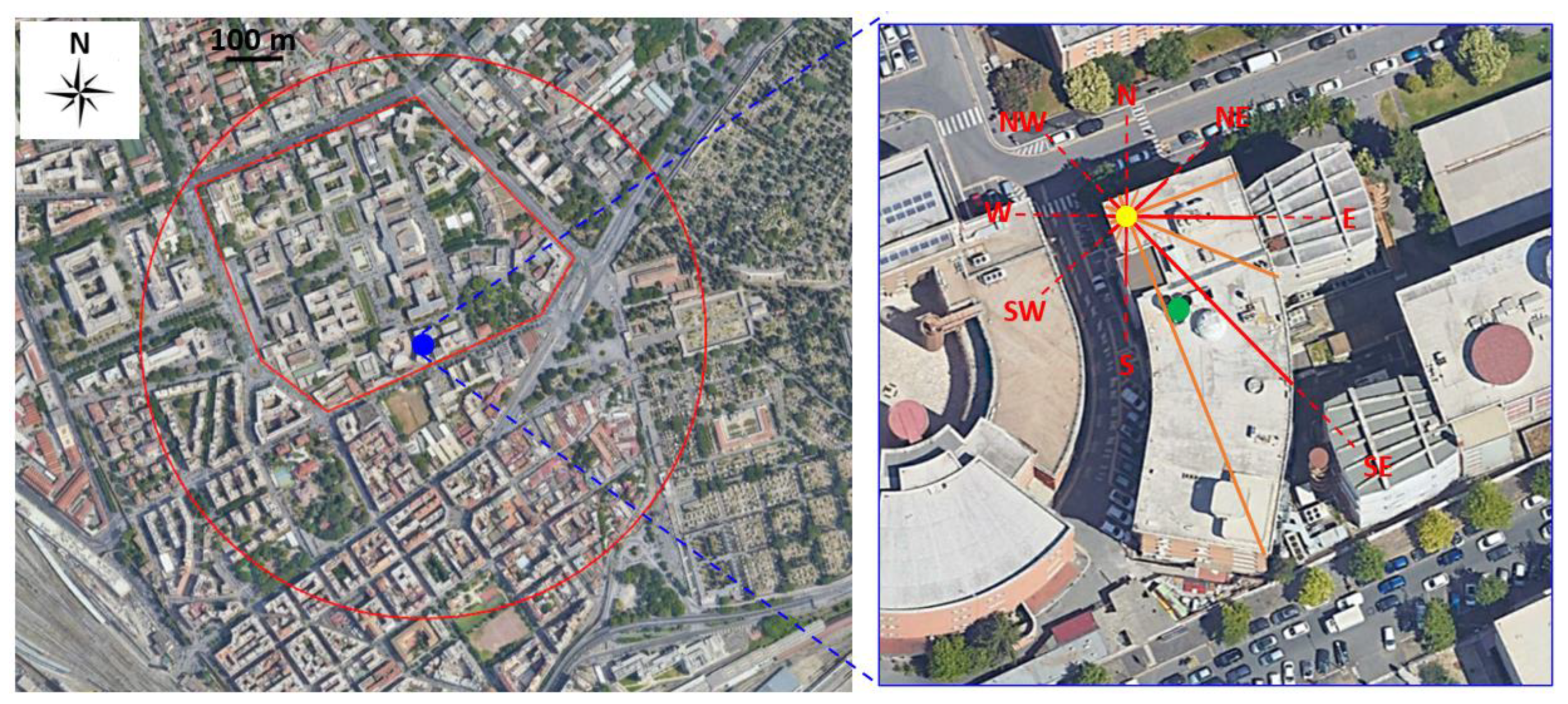
The present work was carried out in the framework of Activity 1 of the VIEPI project, i.e., “Micrometeorological and Indoor Airflow Characterization by Field Experiments and CFD Modeling” [27]. The measurement site was located on the rooftop of the “Fermi” building, belonging to the Physics Department of Sapienza University of Rome (41.902 N, 12.516 E), in a central area of Rome. The left panel of Figure 3 shows an aerial view of the site, where the blue circle denotes the building of interest (an enlargement of the area is depicted on the right panel).
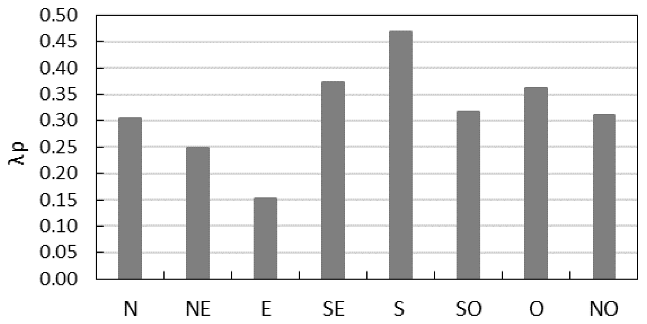
Figure 4 depicts the planar area fraction λ P (i.e., the fraction of the planar area occupied by buildings with respect to the total lot area) as a function of the wind direction. In particular, the average value of λ P in 45° sectors is shown, considering the circled area had a 1 km diameter (red circle in Figure 3) centered over the “Fermi” building. This value was chosen considering that the footprint referred to a representative height equal to 30 m [34,35], with the aim of identifying the upstream area contributing to the measurements of the momentum flux. A map of λ P calculated considering the cells belonging to a uniform grid cell mesh of 50 × 50 m2 covering the area of interest is given in Supplementary Materials (Figure S1). The value of λ P averaged over all directions was 0.3. The highest values occurred for the south and south-east directions because of the presence of the highly built San Lorenzo district, while the lowest λ P occurred for the east direction, which corresponded to the area covered by the Verano cemetery (see Figure 3, left panel).
With regard to the wind field typically observed in the area of interest, slope flows and sea–land breeze circulations affect the city of Rome for large parts of the year, as shown in [7,36,37,38,39]. Two prevalent wind directions can be detected during daytime and night-time, i.e., south-west and north-east, respectively [27].
Measurements were carried out by means of a sonic anemometer/thermometer (Gill Instruments Limited, Lymington, UK) and a three-axial, monostatic Doppler SODAR located on the terrace of the “Fermi” building (Figure 3, right panel). The sonic anemometer was mounted on a 3.5 m mast, i.e., at z/H = 1.15, where H = 24 m is the building height and z is the height above the ground level.
The acoustic bursts of the SODAR (repetition rate 1 s) provided the vertical profiles of wind velocity, wind direction, and standard deviation of the vertical component of the velocity with a vertical resolution of about 5.7 m, ranging from z/H = 1.42 up to z/H = 6.38. Owing to ambient noise, the maximum height was often below z/H = 4.25, while the range gate closest to the terrace was discarded [40,41].

2.3. Data Processing

The measurement campaign was carried out from December 2017 to December 2019. In the present work, data taken during April 2018 were analyzed, for a total amount of about 1440 30 min averages.
The sonic anemometer measured the three wind components and the virtual temperature with a frequency of 32 Hz. The SODAR returned the three velocity components and the standard deviation of the vertical velocity component in the height range 1.42 < z/H < 4.25.
In Table 3, the main variables of interest measured and calculated by the sonic anemometer and the SODAR are listed at the different heights.
The measuring timeslots when the wind direction varied more than 22.5° along the vertical were discarded. Furthermore, friction velocity, Obukhov length, and sensible heat flux ( H s ) were calculated, considering the 30 min averages referred to sonic data at z/H = 1.15. The Obukhov length, the sensible heat flux, and the friction velocity are defined in Equations (2)–(4).
In the present work, L, u * , and H s were calculated for two coordinate systems: the first refers to the geodetic reference system, while the second corresponds to that aligned with the streamlines. In these two coordinate systems, u * , H s and L are expected to be different.
The classification of Holtslag [42] was used to define the stability classes (Table 4), from highly unstable (A) to strongly stable (H), passing through the neutral class (D, defined by the narrow limit of |L| > 500). It is worth emphasizing the same event could belong to a different stability class if calculated from one reference frame rather than the other.

2.3.1. The Normal and Tilted Coordinate Systems

In the tilted coordinate system, the Utilt-axis is aligned with the mean wind velocity, so that Vtilt-axis and Wtilt-axis components of wind velocity are zeros and the Wtilt-axis is transversal to the mean flow. The tilt angle ( φ tilt ) represents the inclination of the mean flow with respect to the horizontal plane. For sake of brevity, the procedure followed for the determination of φ tilt , commonly called “double rotation”, is not reported here. Details can be found in [43].
The rotation of the coordinate system is generally used to remove pseudo quantities when the anemometer is not positioned vertically over a horizontal terrain [14,43,44]. Besides, the rotation of the coordinate system can be used to correct flow distortion caused by measuring equipment, like towers on which anemometers are mounted [26,29]. Lastly, the double rotation is often applied in case of slightly sloping terrain [45]. In this case, the vertical velocity is not expected to be zero and vertical fluxes calculated in a normal coordinate system depend on the terrain slope. Therefore, turbulent fluxes calculated in a tilted coordinate system are more easily comparable to theoretical models (such as MOST) and measurements over flat terrain.
The coordinate system rotation is not generally used when measurements are carried out within the RSL [31,46], in that the mean vertical wind velocity is not expected to be zero due to the presence of the buildings. Nevertheless, we applied the double rotation to data taken within the RSL analogously to what is commonly used in case of sloping terrain.
We hypothesized that turbulent fluxes calculated using the streamline coordinate system could approximate the turbulent fluxes in the CFL.

2.3.2. Estimation of Friction Velocity from SODAR Measurements

In addition to the friction velocities calculated from the sonic anemometer ( u * nrm and u * tilt ), three estimations of friction velocity were carried out using the SODAR data based on the empirical relation c = u / u * , where c is a constant and u is the undisturbed wind velocity. Since no information on u was available from the measured velocity profiles, the latter was estimated applying the profile method [47], originally designed to determine the friction velocity from wind velocity profiles. In the present work, we fit with a logarithmic function every 30 min averaged velocity profile measured by the SODAR in the height range 1.5 < z/H < 3.5. The value of the resulting logarithmic function at z/H = 8 has been assumed as an estimation of the undisturbed velocity for that profile, in that it can be considered well above the building rooftop. It is worth noting that this method is valid irrespective of the stability condition.
Then, three values of the ratio c = u * / u based on laboratory experiments were considered, namely, c = 0.037 by [48], c = 0.047 by [49], and c = 0.052 by [25]. The corresponding friction velocities were u * c = 0.037 , u * c = 0.047 , and u * c = 0.052 , respectively. Since the velocity profiles were classified based on the eight stability categories by Holtslag [40], eight values of u * for each of the three estimated friction velocities were calculated. In this case, the classification of Holtslag was based on the Obukhov length, L nrm , calculated considering the normal coordinate system.

2.3.3. Data Processing for Comparison with Existing MOST Parameterizations

In order to evaluate the applicability of MOST to the RSL above Rome, the measured σ w / u * vertical profiles were compared with those modelled by means of the MOST formulations listed in Table 1.
For each of the 1440 averaged data points available for each height, the stability class was determined considering both L nrm and L tilt . Then, the mean values of u * nrm , L nrm ,   u * tilt , L tilt , and σ w were obtained by averaging them for each stability class. In addition, the three estimated friction velocities for each stability class calculated using the profile method were considered. Therefore, five measured ratios were obtained, i.e., σ w / u * nrm , σ w / u * c = 0.037 , σ w / u * c = 0.047 , σ w / u * c = 0.052 and σ w / u * tilt . In the last case, the classification by Holtslag was based on L tilt . These experimental ratios were compared with the modelled ones, obtained using Equation (5), and the parameters listed in Table 2.
It is worth noting that most of the currently used σ w / u * formulations consider local u * and L as velocity and length scales. In contrast, in the present work, L refers to one single height located at z = 1.15H (i.e., within the RSL), while u * was either measured at z/H = 1.15 by the sonic anemometer or estimated by SODAR data. This procedure is strictly valid only if the measurement point of u * and L and the σ w profiles are within the CFL. However, we aimed to assess the applicability of the available friction velocities ( u * nrm , u * tilt ,   u * c = 0.037 , u * c = 0.047 , and u * c = 0.052 ) and Obukhov lengths ( L nrm and L tilt ) as velocity and length scales. Using the velocity and length scales proposed in this work would make it possible to overcome the difficulties in making measurements of standard deviation and turbulent fluxes at several measuring point or at high altitudes as in the case of the CFL.

3. Results and Discussion

3.1. Sonic Anemometer Measurements

3.1.1. Physical Meaning of the Tilted Coordinate System

Figure 5a shows the tilt angle, φ tilt , as a function of the wind direction. The red points refer to all values, while the red line represents the 20-value moving average of φ tilt . In the secondary axis, the distance between the anemometer and the building edge where the wind impinges for the 16 wind sectors (see Figure 3) is shown. Higher φ tilt occurred when the edge-anemometer distance (dedge) was shorter, while φ tilt was smaller for larger dedge values. This was probably due to the interaction of the wind with the building on which the anemometer was installed. The wind impinging the building tends to flow upward, while over the terrace it gradually returns parallel to the surface (see, e.g., [50] for a comprehensive review on the flow topology in correspondence of groups of buildings). Consequently, if the anemometer is close to the edge, φ tilt can be greater. In contrast, if the anemometer is far from the edge, φ tilt assumes lower values and should tend to zero. Figure 5b shows how the wind returned to almost horizontal after a short distance. In fact, φ tilt increased considerably for dedge values smaller than 5 m, while it remained almost constant for larger dedge values. A similar result was found by [26], where the limit distance was 3 m.

3.1.2. Comparison between Turbulent Fluxes in the Normal and Tilted Coordinate Systems

Friction Velocity

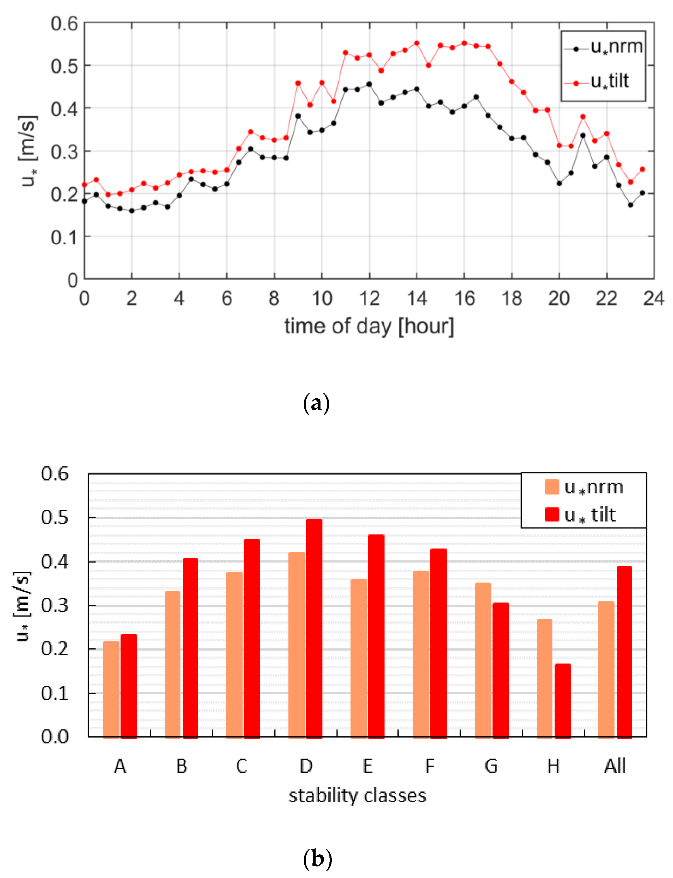
As mentioned in Section 2.3, two estimates of the friction velocity were obtained: the first one using the normal coordinate system, u * nrm , and the second one using the tilted coordinate system, u * tilt . The daily cycle of u * nrm and u * tilt , computed based on data from April 2018, are shown in Figure 6a. Larger values occurred during daytime, in correspondence to the sea breeze coming from south–southwest, while the minimum took place during nighttime. Such a trend is similar to those observed in previous works, e.g., [51,52]. u * tilt behaved similarly to u * nrm , but it showed higher values, particularly during daytime.
Figure 6b shows u * nrm and u * tilt averaged over each stability class. Overall, u * tilt was higher than u * nrm . The values of u * in neutral conditions showed the higher values as a consequence of the stronger winds that characterized the neutral case, while they decreased in the stable and unstable classes. Since very stable conditions occurred rarely, very little data were available in the more stable classes. This makes the reliability of u * nrm and u * tilt for classes G and H quite poor.

Heat Flux

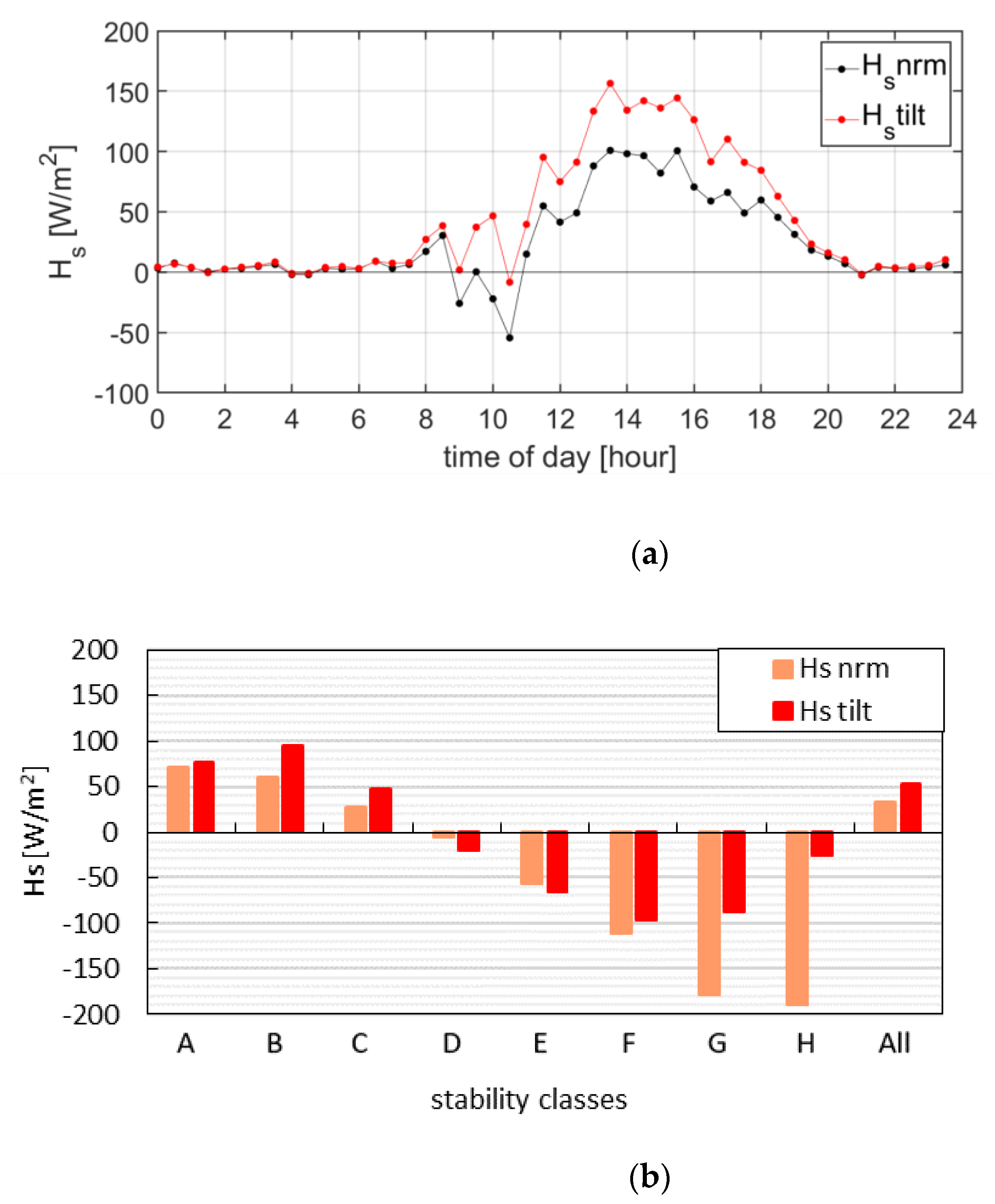
In Figure 7a, the daily cycles of the sensible heat fluxes H s nrm and H s tilt are shown. Both of them were computed from velocity and virtual temperature collected by the sonic anemometer. According to what has usually been found in urban areas [53], their maximum occurs in the early afternoon, while they are generally positive (i.e., upward) during both daytime and nighttime. The main difference between H s nrm and H s tilt regards the higher H s tilt observed in the daytime (nearly 40% in the time interval 12–16).
As shown in Figure 6a and Figure 7a, both momentum and sensible heat fluxes are higher when the tilted coordinate system is used. This is probably due to pseudo fluctuations of velocity along the vertical in the normal coordinate system, as elucidated in Section 3.1.1. When the wind blows horizontally, fluctuations of the vertical component of velocity correspond to fluctuations in the direction transversal to the flow. Instead, when the wind is tilted with respect to the horizontal plane, fluctuations in the two directions transversal and longitudinal to the flow are mixed. This gives rise to fluctuations of the vertical velocity component. No pseudo fluctuations exist when the tilted coordinate system is used. Nightime H s tilt ~ H s nrm because the heat flux is around zero in these hours.
The mean values of H s nrm and H s tilt for each stability class are depicted in Figure 7b. As expected, positive heat fluxes occurred for unstable conditions, while they were negative for stable conditions; neutral conditions were characterized by values close to zero.
Hourly averaged friction velocity and sensible heat flux along with the percentage difference between the quantities in the tilted and normal coordinate systems are shown in Table S1 in the Supplementary Materials.
Figure 7a shows a negative heat flux in the period 9:00–11:00. Such an anomalous trend is ascribable to strong winds and large negative heat fluxes that occurred on April 9th. This day has been included in the monthly averages shown in Figure 7a; in Figure S2 in the Supplementary Material, the mean daily trends of heat fluxes and friction velocity calculated excluding April 9th are reported.

Obukhov Length

In Figure 8, the frequency of occurrence (F%) of the stability classes based on the classification reported in Table 4 is shown. The Obukhov length has been calculated using Equation (2). Overall, most of the time was characterized by unstable conditions (classes A and B), while only very little data corresponding to the stable classes were observed.
Since both friction velocity and sensible heat flux depend on the coordinate system on which they are calculated, the statistics in each stability class are different when either the normal or the tilted coordinate system is used. The frequency of occurrence of classes from B to E increases if the classification is based on L tilt .
As expected, unstable conditions occurred more frequently during daytime, while stable conditions characterized the nocturnal period. Given the absence of strong winds during the investigated period, neutral conditions were generally present during the two day–night transitions (sunrise and sunset). However, unstable conditions always prevailed, even at night. This is a consequence of the positive sign (upward) of the sensible heat flux measured during the nighttime. This phenomenon, typically observed in urban areas [29,51], can be ascribed to the continuous release in the afternoon and at night of the heat absorbed daytime by the construction materials [54,55].

3.2. Estimation of Friction Velocity from SODAR Measurements

As mentioned in Section 2.3, three friction velocity estimates were conducted using the SODAR data in addition to those calculated using sonic anemometer data ( u * nrm and u * tilt ). The vertical profiles of the wind velocity (30–min average) were fitted with a logarithmic function. For each of these, an undisturbed wind velocity ( u ) was calculated by the velocity value modelled at z/H = 8, considering the log law (see Section 1). Since the performances of the logarithmic profiles were rather high (Table S2), the estimation of the asymptotic wind speeds can be considered quite reliable.
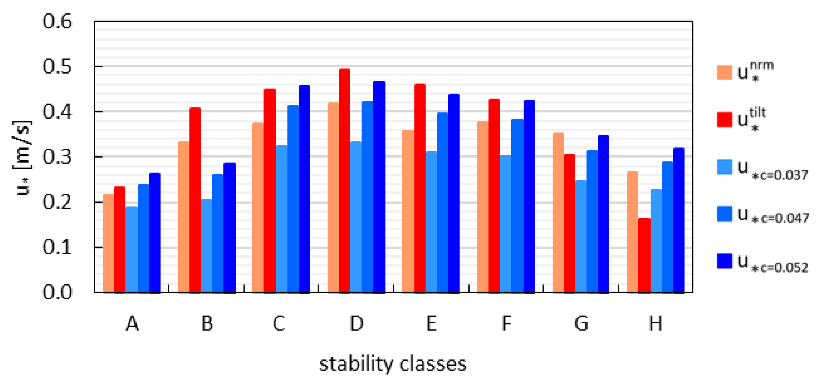
Based on the three estimations of c = u * / u found in the literature (c = 0.037, 0.047, 0.052, see Section 2.3.2), three different friction velocities were obtained, viz.: u * c = 0.037 , u * c = 0.047 and u * c = 0.052 . Therefore, eight averaged values of u * c = 0.037 , u * c = 0.047 , and u * c = 0.052 , one per stability class, were calculated. The results, including the two estimations carried out by using the sonic anemometer as described in Section 3.1.2, are shown in Figure 9. These three friction velocities showed the same trend followed by u * nrm and u * tilt , i.e., the highest values occurred in neutral conditions, while they decreased for the stable or unstable classes. This suggests that the estimation method works quite well. However, the method is strictly valid only for the neutral case, in that the three u * / u considered in the present study refer to neutral conditions.
Except for classes G and H, where the results must be seen with circumspection because of the small amount of data used to build the statistics, u * c = 0.037 was always the smallest. The greatest difference between the estimated and the measured friction velocities occurred for class B. In particular, the percentage difference between the measured (average of u * nrm and u * tilt ) and the estimated (average of u * c = 0.037 , u * c = 0.047 , u * c = 0.052 ) friction velocities was 33% for class B and 29% for class H, while it was below 11% elsewhere.

3.3. Applicability of MOST in the Roughness Sublayer above Rome

The measured σ w / u * vertical profiles were compared with the modelled ones for each stability class. As described in Section 2, the non-dimensional quantities σ w / u * nrm , σ w / u * tilt , σ w / u * c = 0.037 ; σ w / u * c = 0.047 ,   and   σ w / u * c = 0.052 as a function of z / L nrm (or z / L tilt when the tilted coordinate system is considered) have been obtained. The modelled σ w / u * at various heights were calculated for each stability class using Equation (5) and L nrm (or L tilt ). Here, seven MOST formulations were tested in accordance with Table 1. It is worth noting that only one value of friction velocity and Obukhov length was assumed for the whole σ w vertical profile.
For each stability class, the relative difference (E%) was computed as follows:
E % ( Ref ,   u * j ; z i / H ) = | σ w u * j ( Exp ; z i H ) σ w u * j ( Ref ; z i H ) | σ w u * j ( Exp ; z i H ) · 100
where Ref and Exp refer to the modelled and experimental σ w / u * profiles, respectively. E% was calculated for each dimensionless height ( z i / H ) and for the five friction velocity formulations ( u * j ).
By averaging the relative difference at various heights, the mean relative difference for each stability class was found:
E %   ¯ ( Ref ,   u * j ) = 1 N z i = 1 N z E % ( Ref ,   u * j ; z i / H )
while averaging the relative difference for all the stability classes, the overall relative difference was obtained.

3.3.1. Applicability of MOST Considering Each Stability Class

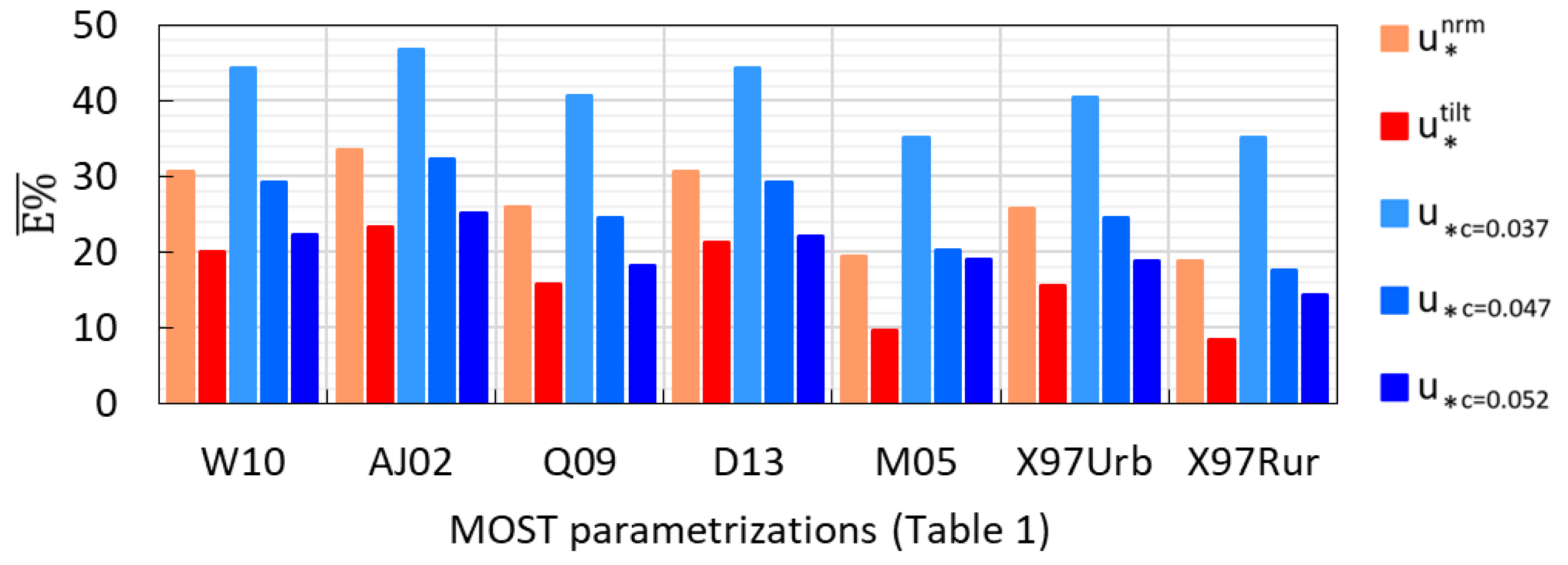
The comparison among all E % ¯ calculated considering our experimental data and the MOST formulations listed in Table 1 is shown in Figure 10. Note that results referring to the more stable classes (G and H) are not presented due to the lack of data.
The relative difference for each tested formulation varied with the stability class. Besides, the performances changed considering the different friction velocities.
Overall, W10 showed the best performances for neutral (D) and slightly stable (E, F) classes. AJ02 and Q09 showed low relative differences for the slightly stable classes, considering all the friction velocities tested. In general, X97Rur, X97Urb, D13, and M05 showed the best performances for slightly stable and very unstable classes (A), while they returned higher relative differences for unstable, slightly unstable, and neutral classes.
Considering the very unstable class (A), u * c = 0.052 gave the best results (except for M05 and X97Rur). Since u * c = 0.052 showed the highest value, the other friction velocities probably underestimated the real one. M05 and X97Rur showed the best performances when u * nrm and u * c = 0.047 were considered. From unstable (B) to neutral (D) conditions, u * tilt seemed to give the lowest difference. This means that the friction velocities estimated using the SODAR measurements for class B were too small. For class C, the results given by u * tilt and u * c = 0.052 were very similar, as the two quantities are comparable. u * tilt returned very low relative differences in class D for W10, Q09, AJ02, and X97Rur formulations. Looking at class E, the best results corresponded to u * c = 0.052 , followed by u * tilt . For class F, the best performances were obtained with u * c = 0.052 ,   u * c = 0.047 , or u * nrm , depending on the formulation.

3.3.2. Overall Applicability of MOST

Figure 11 shows the overall relative difference for each tested MOST formulation. This assessment is useful to understand which are the best MOST formulations and the scaling variables that work better, considering all the stability conditions.
Overall, u * tilt gave the smallest relative difference for all the formulations tested here. The worst results were given by u * c = 0.037 . The overall relative difference given by u * tilt considering all the formulations was below 24%. However, as shown in Section 3.3.1, a certain degree of variability exists among the stability classes. The maximum and minimum relative difference obtained with u * tilt were 42.7% (very unstable, formulation W10) and 1.4% (unstable, formulation X97Rur).
The lowest overall relative difference was obtained when using u * tilt as velocity scale, L tilt as length scale, and the formulation X97Rur (8.4%). Very good performances were obtained when using u * tilt , L tilt , and M05 too (9.6%). The comparison was good also with the other formulations. Among the existing formulations tested in this work, terrain conditions most similar to Rome were obtained by AJ02. The overall relative difference was 23.4% when considering u * tilt (and L tilt ) and the formulation AJ02. Particularly good results were obtained with this formulation and this velocity and length scale in neutral and slightly stable stability conditions.
The results obtained in this work suggest that u * tilt and L tilt , measured at a sole height within the RSL (z/H = 1.15), can be used as velocity and length scales for the whole vertical profile. This makes it possible to overcome the difficulties in taking measurements of turbulent fluxes either at several heights or at an altitude high enough to be in the constant flux layer.

4. Conclusions

In the present work, wind and temperature data, collected by a sonic anemometer and a three-axial monostatic Doppler SODAR in the framework of the VIEPI project during April 2018, have been used to test the applicability of MOST parametrizations above Rome. Seven parametrizations of the ratio σ w / u * as a function of z / L taken from the literature were considered. Furthermore, two coordinate systems, named normal and tilted, have been tested. The normal coordinate system is aligned with the geographical one, while the tilted follows the streamlines of the mean flow. For both coordinate systems, the main turbulence scaling parameters, i.e., L , u * , H s , and the stability class, were computed. In particular, L tilt and L nrm were tested as length scales, while u * nrm , u * tilt , u * c = 0.037 , u * c = 0.047 , and u * c = 0.052 were tested as velocity scales. All the previous quantities followed the expected trends with time of day and stability conditions.
One of the most relevant result suggests that it is possible to assume a unique value of u * and L as representative of the entire σ w vertical profile, albeit the investigated point was below the CFL. This result is important since, in the literature, the MOST has typically been used above urban areas either in the CFL (classical MOST) or in the RSL and in the ML, using local u * and L as scaling quantities (local MOST). However, the application of MOST according with literature could be very complex in realistic cases as they require the measurement of turbulent fluxes at several heights and the installation of the instrument within the CFL. The new formulation proposed here seems to overcome these problems, allowing the application even outside the CFL.
Regarding the results of the two coordinate systems, both thermal and mechanical fluxes in the tilted coordinate system showed higher values than in the normal system. The friction velocities estimated by the SODAR data, u * c = 0.037 , u * c = 0.047 and u * c = 0.052 , followed the same trend, varying both the stability conditions and the measured friction velocities ( u * tilt and u * nrm ). This suggests that the proposed method to reconstruct the values of u * can be applied successfully, fixing a priori the correct u * / u ratio.
Finally, the applicability of the MOST in urban area has been tested by comparing, for each stability class, the measured and modelled σ w / u * ratios as a function of z / L . The comparison has been carried out for seven theoretic MOST parametrizations, setting the various friction velocities and Obukhov lengths as velocity and length scales, respectively. The best performances were obtained when u * tilt and L tilt were used as velocity and length scales, along with the formulation by X97Rur. Considering all the stability classes, the relative difference was 8.4%. However, the overall relative difference given by u * tilt was lower than 24%, considering all the investigated formulations. This suggests that the existing MOST formulations can be considered valid for our case study, if u * tilt and L tilt are used as velocity and length scales.
This study demonstrated that using u * tilt and L tilt as scaling parameters, it would be possible to overcome the difficulties in carrying out measurements of turbulent fluxes at different quotes or at an altitude high enough to be in the constant flux layer. The proposed methodology is new and represents a first step which, requires further testing both in other sites and at the laboratory scale, given the complexity and the great variability of the flow pattern occurring in urban areas.
Finally, the present results can be considered as the starting point for further development of a formulation allowing the extension of the MOST below the CFL and, therefore, to estimate the profiles of meteorological variables also within the urban canyons.
Furthermore, in relationship with the relevance of micro-meteorology for the indoor exposure, a hypothetical calculation of the micro-meteorological profiles inside an urban canyon can be useful to evaluate the pressure field in proximity to the indoor environments of the investigated building, and to better evaluate the dispersion of pollutants emitted by vehicular traffic and domestic heating.

Supplementary Materials

The following are available online at https://www.mdpi.com/article/10.3390/su13158426/s1, Figure S1: Planar area fraction, 50 m × 50 m grid, Figure S2: Daily trend of turbulent sensible heat fluxes and friction velocity. Each point is the monthly average of heat fluxes or friction velocity at the time of day. April 9th has been excluded as an extreme event occurred, Table S1: Hourly averaged values of friction velocity and sensible heat flux along with the percentage difference between the quantities in the tilted and normal coordinate systems, Table S2: Parameters of the logarithmic fit of the wind velocity vertical profile per each atmospheric stability class. The logarithmic function used is the following: u = α ln ( z H ) + β (where z is the height a.g.l., H is the building height and u is the wind velocity).

Author Contributions

Conceptualization: A.P.; methodology: A.P.; investigation: L.G. and A.P.; data curation: A.D.B., L.G. and A.P.; writing—original draft: L.G. and A.P.; writing—review and editing: A.D.B.; supervision: A.P.; project administration: A.P. All authors have read and agreed to the published version of the manuscript.

Funding

This research was carried out in the frame of INAIL (Italian Workers’ Compensation Authority) institutional researches.

Institutional Review Board Statement

Not applicable.

Informed Consent Statement

Not applicable.

Data Availability Statement

Not applicable.

Acknowledgments

The authors gratefully acknowledge Marco Cacciani and the BAQUNIN team for hosting and supporting part of the experimental campaign and for providing SODAR data.

Conflicts of Interest

The authors declare no conflict of interest.

References

  1. Pasquill, F. Atmospheric Diffusion, 2nd ed.; Halstead Press: New York, NY, USA, 1974. [Google Scholar]
  2. Stull, R.B. An Introduction to Boundary Layer Meteorology; Kluwer Academic Publisher: Dordrecht, The Netherlands, 1988. [Google Scholar]
  3. Buckingham, E. On physically similar sistems: Illustration of the use of dimensional equations. Phys. Rev. 1914, 4, 345–376. [Google Scholar] [CrossRef]
  4. Monin, A.S.; Obukhov, A.M. Basic Laws of Turbulent Mixing in the Atmosphere near the Ground. Trudy Geofiz. Inst. 1954, 24, 163–187. [Google Scholar]
  5. Foken, T. 50 years of the Monin–Obukhov similarity theory. Bound. Layer Meteorol. 2006, 119, 431–447. [Google Scholar] [CrossRef]
  6. Oke, T.R. The energetic basis of the urban heat island. Q. J. R. Meteorol. Soc. 1982, 108, 1–24. [Google Scholar] [CrossRef]
  7. Di Bernardino, A.; Iannarelli, A.M.; Casadio, S.; Mevi, G.; Campanelli, M.; Casasanta, G.; Cede, A.; Tiefengraber, M.; Siani, A.M.; Cacciani, M. On the Effect of Sea Breeze Regime on Optical and Physical Aerosol Properties in the Urban Area of Rome, Italy. Urban Clim. 2021, 37, 100842. [Google Scholar] [CrossRef]
  8. Fernando, H.J.S.; Lee, S.M.; Anderson, J.; Princevac, M.; Pardyjak, E.; Grossman-Clarke, S. Urban Fluid Mechanics: Air circulation and contaminant dispersion in cities. Environ. Fluid Mech. 2001, 1, 107–164. [Google Scholar] [CrossRef]
  9. Christen, A.; Vogt, R. The energy balance of a central European City. Int. J. Climatol. 2004, 24, 1395–1421. [Google Scholar] [CrossRef]
  10. Barlow, J.F. Progress in observing and modelling the urban boundary layer. Urban Clim. 2014, 10, 216–240. [Google Scholar] [CrossRef] [Green Version]
  11. Giovannini, L.; Zardi, D.; De Franceschi, M. Characterization of the thermal structure inside an urban canyon: Field measurements and validation of a simple model. J. Appl. Meteorol. Climatol. 2013, 52, 64–81. [Google Scholar] [CrossRef]
  12. Conigliaro, E.; Monti, P.; Leuzzi, G.; Cantelli, A. A three-dimensional urban canopy model for mesoscale atmospheric simulations and its comparison with a two-dimensional urban canopy model in an idealized case. Urban Clim. 2021, 37, 100831. [Google Scholar] [CrossRef]
  13. Rotach, M.W. On the influence of the urban roughness sublayer on turbulence and dispersion. Atmos. Environ. 1999, 33, 4001–4008. [Google Scholar] [CrossRef]
  14. Dyer, A.J.; Hicks, B.B. Flux-gradient relationships in the constant flux layer. Q. J. R. Meteorol. Soc. 1970, 96, 715–721. [Google Scholar] [CrossRef]
  15. Arnfield, A.J. Two decades of urban climate research: A review of turbulence, exchanges of energy and water, and the urban heat island. Int. J. Climatol. 2003, 23, 1–26. [Google Scholar] [CrossRef]
  16. Britter, R.E.; Hanna, S.R. Flow and dispersion in urban areas. Annu. Rev. Fluid Mech. 2003, 35, 469–496. [Google Scholar] [CrossRef]
  17. Grimmond, C.S.B.; Oke, T.R. Aerodynamic properties of urban areas derived from analysis of urban surface form. J. Appl. Meteorol. 1999, 38, 1261–1292. [Google Scholar] [CrossRef]
  18. Rotach, M.W. Structure of the Urban Boundary Layer. In COST 715 Final Report: Meteorology Applied to Urban Air Pollution Problems; Fisher, B., Joffre, S., Kukkonen, J., Piringer, M., Rotach, M., Schatzmann, M., Eds.; Demetra Ltd Publishers: Sofia, Bulgaria, 2005. [Google Scholar]
  19. Dallman, A.; Di Sabatino, S.; Fernando, H.J.S. Flow and turbulence in an industrial/suburban roughness canopy. Environ. Fluid Mech. 2013, 13, 279–307. [Google Scholar] [CrossRef]
  20. Pelliccioni, A.; Monti, P.; Leuzzi, G. Wind-Speed Profile and Roughness Sublayer Depth Modelling in Urban Boundary Layers. Bound. Layer Meteorol. 2016, 160, 225–248. [Google Scholar] [CrossRef]
  21. Kastner-Klein, P.; Rotach, M.W. Mean flow and turbulence characteristics in an urban roughness sublayer. Bound. Layer Meteorol. 2004, 111, 55–84. [Google Scholar] [CrossRef]
  22. Zajic, D.; Fernando, H.J.S.; Brown, M.J.; Pardyjak, E.R. On flows in simulated urban canopies. Environ. Fluid Mech. 2015, 15, 275–303. [Google Scholar] [CrossRef]
  23. Di Bernardino, A.; Monti, P.; Leuzzi, G.; Querzoli, G. Pollutant fluxes in two-dimensional street canyons. Urban Clim. 2018, 24, 80–93. [Google Scholar] [CrossRef]
  24. Coceal, O.; Thomas, T.G.; Castro, I.P.; Belcher, S.E. Mean flow and turbulence statistics over groups of urban-like obstacles. Bound. Layer Meteorol. 2006, 121, 491–519. [Google Scholar] [CrossRef]
  25. Di Bernardino, A.; Monti, P.; Leuzzi, G.; Querzoli, G. Turbulent Schmidt number measurements over three-dimensional cubic arrays. Bound. Layer Meteorol. 2020, 174, 231–250. [Google Scholar] [CrossRef] [Green Version]
  26. Barlow, J.F.; Dobre, A.; Smalley, R.J.; Arnolds, S.J.; Tomlin, A.S.; Belcher, S.E. Referencing of street-level flows measured during the DAPPLE 2004 campaign. Atmos. Environ. 2009, 43, 5536–5544. [Google Scholar] [CrossRef]
  27. Pelliccioni, A.; Monti, P.; Cattani, G.; Boccuni, F.; Cacciani, M.; Canepari, S.; Capone, P.; Catrambone, M.; Cusano, M.; D’Ovidio, M.C.; et al. Integrated Evaluation of Indoor Particulate Exposure: The VIEPI Project. Sustainability 2020, 12, 9758. [Google Scholar] [CrossRef]
  28. Foken, T. Micrometeorology; Springer: Berlin/Heidelberg, Germany, 2008. [Google Scholar]
  29. Wood, C.R.; Lacser, A.; Barlow, J.F.; Padhra, A.; Belcher, S.E.; Nemitz, E.; Helfter, C.; Famulari, D.; Grimmond, C.S.B. Turbulent Flow at 190 m Height above London during 2006–2008: A Climatology and the Applicability of Similarity Theory. Bound. Layer Meteorol. 2010, 137, 77–96. [Google Scholar] [CrossRef] [Green Version]
  30. Al-Jiboori, M.H.; Xu, Y.; Qian, Y. Local Similarity Relationships in the Urban Boundary Layer. Bound. Layer Meteorol. 2002, 102, 63–82. [Google Scholar] [CrossRef]
  31. Quan, L.; Hu, F. Relationship between turbulent flux and variance in the urban canopy. Meteorol. Atmospheric Phys. 2009, 104, 29–36. [Google Scholar] [CrossRef]
  32. Xu, Y.; Zhou, C.; Li, Z. Turbulent structure and local similarity in the tower layer over the nanjing area. Bound. Layer Meteorol. 1997, 82, 1–21. [Google Scholar]
  33. Moraes, O.L.L.; Acevedo, O.C.; Degrazia, G.A.; Anfossi, D.; da Silva, R.; Anabor, V. Surface layer turbulence parameters over a complex terrain. Atmos. Environ. 2005, 39, 3103–3112. [Google Scholar]
  34. Hsieh, C.-I.; Katul, G.; Chi, T.-W. An approximate analytical model for footprint estimation of scalar fluxes in thermally stratified atmospheric flows. Adv. Water Resour. 2000, 23, 765–772. [Google Scholar] [CrossRef]
  35. Kljun, N.; Rotach, M.W.; Calanca, P. A Simple Parameterisation for Flux Footprint Predictions. Bound. Layer Meteorol. 2004, 112, 503–523. [Google Scholar] [CrossRef]
  36. Pelliccioni, A.; Monti, P.; Leuzzi, G. An alternative wind profile formulation for urban areas in neutral conditions. Environ. Fluid Mech. 2015, 15, 135–146. [Google Scholar] [CrossRef] [Green Version]
  37. Di Bernardino, A.; Iannarelli, A.M.; Casadio, S.; Perrino, C.; Barnaba, F.; Tofful, L.; Campanelli, M.; Di Liberto, L.; Mevi, G.; Cacciani, M. Impact of synoptic meteorological conditions on air quality in three different case studies in Rome, Italy. Atmos. Pollut. Res. 2021, 12, 76–88. [Google Scholar] [CrossRef]
  38. Leuzzi, G.; Monti, P. Breeze Analysis by Mast and Sodar Measurements. Il Nuovo Cimento 1997, C20, 343–359. [Google Scholar]
  39. Monti, P.; Leuzzi, G. A Numerical Study of Mesososcale Airflow and Dispersion over Coastal Complex Terrain. Int. J. Environ. Pollut. 2005, 25, 239–250. [Google Scholar] [CrossRef]
  40. Mastrantonio, G.; Fiocco, G. Accuracy of wind velocity determinations with Doppler sodars. J. Appl. Meteorol. 1982, 21, 823–830. [Google Scholar] [CrossRef]
  41. Mastrantonio, G.; Argentini, S.; Viola, A. A new PC-based real system to analyze sodar echoes. In Proceedings of the 5th Workshop Italia Research on Antarctic Atmosphere, Porano, Italy, 19–21 October 1992; pp. 227–235. [Google Scholar]
  42. Holtslag, A.A.M. Estimates of diabatic wind speed profiles from near-surface weather observations. Bound. Layer Meteorol. 1984, 29, 225–250. [Google Scholar] [CrossRef]
  43. Wilczak, J.M.; Oncley, S.P.; Stage, S.A. Sonic Anemometer Tilt Correction Algorithms. Bound. Layer Meteorol. 2001, 99, 127–150. [Google Scholar] [CrossRef]
  44. Bonacquisti, V. Anemometria Sonica per la Determinazione dei Flussi Turbolenti e Caratterizzazione dello Strato Limite Planetario in Ambiente Urbano. Ph.D. Thesis, Sapienza University of Rome, Rome, Italy, 2008. [Google Scholar]
  45. Nakai, T.; Shimoyama, K. Ultrasonic anemometer angle of attack errors under turbulent conditions. Agric. For. Meteorol. 2012, 162–163, 14–26. [Google Scholar]
  46. Christen, A. Atmospheric Turbulence and Surface Energy Exchange in Urban Environments: Results from the Basel Urban Boundary Layer Experiment (BUBBLE). Ph.D. Thesis, University of Basel, Basel, Switzerland, 2005. [Google Scholar]
  47. Businger, J.A.; Wyngaard, J.C.; Izumi, Y.; Bradley, E.F. Flux-profile relationships in the atmospheric surface layer. Int. J. Atmos. Sci. 1971, 28, 181–189. [Google Scholar] [CrossRef]
  48. Nironi, C.; Salizzoni, P.; Marro, M.; Mejean, P.; Grosjean, N.; Soulhac, L. Dispersion of a Passive Scalar Fluctuating Plume in a Turbulent Boundary Layer. Part I: Velocity and Concentration Measurements. Bound. Layer Meteorol. 2015, 156, 415–446. [Google Scholar] [CrossRef]
  49. Fackrell, J.E.; Robins, A.G. Concentration fluctuations and fluxes in plumes from point sources in a turbulent boundary layer. J. Fluid Mech. 1982, 117, 1–26. [Google Scholar] [CrossRef]
  50. Nardecchia, F.; Di Bernardino, A.; Pagliaro, F.; Monti, P.; Leuzzi, G.; Gugliermetti, L. CFD analysis of urban canopy flows employing the V2F model: Impact of different aspect ratios and relative heights. Adv. Meteorol. 2018, 2018. [Google Scholar] [CrossRef]
  51. Pelliccioni, A.; Monti, P.; Gariazzo, C. Some characteristics of the urban boundary layer above Rome, Italy, and applicability of Monin–Obukhov similarity. Environ. Fluid Mech. 2012, 12, 405–428. [Google Scholar] [CrossRef]
  52. De Ridder, K. Bulk Transfer Relations for the Roughness Sublayer. Bound. Layer Meteorol. 2010, 134, 257–267. [Google Scholar] [CrossRef]
  53. Oke, T.R.; Mills, G.; Christen, A.; Voogt, J.A. Urban Climates; Cambridge University Press: Cambridge, UK, 2017. [Google Scholar]
  54. Masson, V. A physically-based scheme for the urban energy budget in atmospheric models. Bound. Layer Meteorol. 2000, 94, 357–397. [Google Scholar] [CrossRef]
  55. Cantelli, A.; Monti, P.; Leuzzi, G. Numerical study of the urban geometrical representation impact in a surface energy budget model. Environ. Fluid Mech. 2015, 15, 251–273. [Google Scholar] [CrossRef]
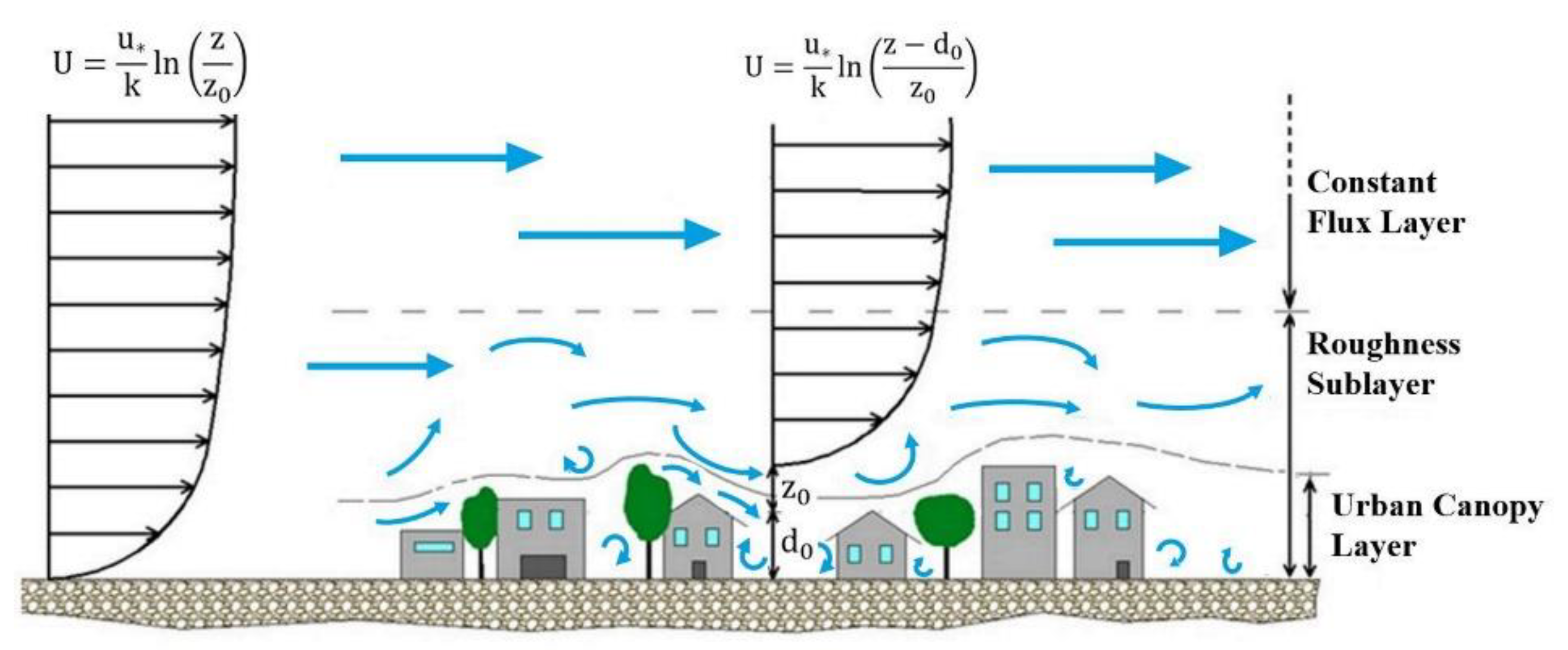
Figure 1. Vertical structure of the ABL in urban environment.
Sustainability 13 08426 g001
Figure 2. σ w / u * as a function of z/L modelled by means of Equation (5) and the parameters listed in Table 2. z ref = 3 h b was been fixed, while 1/L ranged between −0.15 and 0.15.
Sustainability 13 08426 g002
Figure 3. (Left): Aerial view (source: Google Earth) of the Sapienza University Campus. The blue circle indicates the sampling site (”Fermi”). The red polygon indicates the borders of the Sapienza University Campus of Rome. The red circle depicts the area of 500 m in radius. (Right): Enlargement of the region surrounding the “E. Fermi” building. In the right panel, the yellow and green circles refer to the sonic anemometer and the SODAR locations, respectively. For ease of interpretation, the wind sectors have been also depicted.
Sustainability 13 08426 g003
Figure 4. Planar area fraction versus direction.
Sustainability 13 08426 g004
Figure 5. (a) Tilt angle φ tilt (light red circles), its moving average over 20 values (red line), and edge-anemometer distance (blue points) as a function of wind direction. (b) φ tilt as a function of edge–anemometer distance; the orange lines represent the mean φ tilt for edge < 5 m and for edge > 5 m.
Sustainability 13 08426 g005
Figure 6. (a) Daily cycles of friction velocity in the normal (black) and tilted (red) coordinate systems for April 2018. (b) Mean value of friction velocity in the normal (orange) and tilted (red) coordinate systems per each stability class.
Sustainability 13 08426 g006
Figure 7. (a) Daily trend of sensible heat flux in the normal (black) and tilted (red) coordinate system (b) Mean value sensible heat flux in the normal (orange) and tilted (red) coordinate system per each atmospheric stability class.
Sustainability 13 08426 g007
Figure 8. Frequency of occurrence of each stability class, considering the classification based on either L tilt (red) or L nrm (orange).
Sustainability 13 08426 g008
Figure 9. Friction velocities estimated by SODAR data per atmospheric stability class (blue tones), along with friction velocities obtained by sonic anemometer measurements (red tones).
Sustainability 13 08426 g009
Figure 10. Mean relative difference between modelled and experimental σ w / u * ratios, for each stability class.
Sustainability 13 08426 g010
Figure 11. Mean relative difference between modelled and experimental σ w / u * ratios (average value for all the stability classes).
Sustainability 13 08426 g011
Table 1. Overview of the seven MOST parameterizations for standard deviation of vertical wind velocity above urban areas or complex terrain considered in the present study.
AuthorSitehm [m]z0 [m]d0 [m]z [m]Layer of Measuring
Wood (2010)
W10
urban area (London)8.8 ± 3.00.87 ± 0.484.3 ± 1.9190.3CFL or above
Al-Jiboori (2002)
AJ02
urban area (Beijing)n.a.~3.9~2247, 140, 280CFL, RSL, above CFL
Quan (2009)
Q09
urban area (Beijing)n.a.1.7540.1247UCL
Dallman (2013)
D13
suburban area (Phoenix)3.54 ÷ 13.130.04 ÷ 0.180.52 ÷ 4.33~15CFL
Moraes (2005)
M05
rural site (rice plantation in a valley)n.a.n.a.n.a.10CFL
Xu (1997)
X97Urb
urban area (Nanjing)80.63n.a.10, 20, 30, 40, 50RSL, CFL
Xu (1997)
X97Rur
rural area (Baguazhou)n.a.0.035n.a.16, 40, 64, 88, 116, 164CFL
Table 2. Parameters a, b, and p of Equation (5) for the seven MOST parameterizations listed in Table 1.
AuthorsAtmospheric Stabilityabp
W10Unstable1.31−0.651/3
Stable1.400.460.19
AJ02Unstable1.22−1.051/3
Stable1.221.051/3
Q09Unstable1.33−1.271/3
Stable1.420.541/3
D13Unstable0.98−5.641/3
Stable1.350.551/3
M05Unstable1.2−5.31/3
Stable1.24.31/3
X97UrbUnstable1.23−2.301/3
Stable1.232.801/3
X97RurUnstable1.35−3.101/3
Stable1.351.301/3
Table 3. Variables obtained by the sonic anemometer and SODAR data along with the corresponding dimensionless measuring heights.
InstrumentsVariablesDimensionless Measuring Height
Sonic anemometer
Meridional wind ( U )z/H = 1.15
Zonal wind (V)
Vertical wind (W)
Virtual temperature ( T v )
Standard deviation of vertical wind ( σ w )
Sensible heat turbulent flux in the normal and tilted coordinate system ( H s nrm   and   H s tilt )
Friction velocity in the normal and tilted coordinate system ( u * nrm   and   u * tilt )
Obukhov length in the normal and tilted coordinate system ( L nrm   and   L tilt )
Wind direction
Tilt angle ( φ tilt )
SODARMeridional wind ( U )1.42 < z/H < 4.25
Zonal wind ( V )
Vertical wind ( W )
Standard deviation of vertical wind ( σ w )
Table 4. Classification of Holtslag in eight atmospheric stability classes.
Stability ClassObukhov Length Range
A 40 <   L   < 0
B 200 <   L   < 40
C 500 <   L   < 200
D | L | > 500
E 200 <   L   < 500
F 100 <   L   < 200
G 40 <   L   < 100
H 0 <   L   < 40
Publisher’s Note: MDPI stays neutral with regard to jurisdictional claims in published maps and institutional affiliations.