A Factorial Ecological-Extended Physical Input-Output Model for Identifying Optimal Urban Solid Waste Path in Fujian Province, China

Abstract

Effective management of an urban solid waste system (USWS) is crucial for balancing the tradeoff between economic development and environment protection. A factorial ecological-extended physical input-output model (FE-PIOM) was developed for identifying an optimal urban solid waste path in an USWS. The FE-PIOM integrates physical input-output model (PIOM), ecological network analysis (ENA), and fractional factorial analysis (FFA) into a general framework. The FE-PIOM can analyze waste production flows and ecological relationships among sectors, quantify key factor interactions on USWS performance, and finally provide a sound waste production control path. The FE-PIOM is applied to managing the USWS of Fujian Province in China. The major findings are: (i) waste is mainly generated from primary manufacturing (PM) and advanced manufacturing (AM), accounting for 30% and 38% of the total amount; (ii) AM is the biggest sector that controls the productions of other sectors (weight is from 35% to 50%); (iii) the USWS is mutualistic, where direct consumption coefficients of AM and PM are key factors that have negative effects on solid waste production intensity; (iv) the commodity consumption of AM and PM from other sectors, as well as economic activities of CON, TRA and OTH, should both decrease by 20%, which would be beneficial to the sustainability of the USWS.

1. Introduction

1.1. Importance and Motivation

With rapid urbanization and industrialization, humans consume increasing goods and services which cause the growth of direct and indirect urban solid waste generation [1]. Urban solid waste often has harmful impacts on human health and the ecological environment. Urban solid waste management, regarding the treatment of solid, liquid and/or atmospheric wastes before they are released into the environment is an issue of growing global concern [2]. In China, solid waste generation shows a trend of growth, and the corresponding utilization-disposal rate is trending downward. In 2011, the amounts of industrial solid waste and household garbage reached 3.62 billion and 0.16 billion Mg, respectively. The disposal rate and utilization rate were about 25.88% and 54.24%, respectively. In 2019, the amounts of industrial solid waste and household garbage increased to 3.86 billion and 0.24 billion Mg, respectively, whereas the disposal rate and utilization rate were about 24.31% and 53.33%, respectively. Investment in environmental protection occupied about 1.21% of GDP, while investment in solid waste production was much less [3]. Strategies that can help reduce the negative impacts of large amount of urban solid waste are desired [4].

The formulation of sound strategies requires the cooperation of numerous economic sectors [5]. When considering the city as a complex system, various economic sectors have direct or indirect relationships. The urban system can be treated as a network in which sectors are comparable to nodes and intersectoral transactions correspond to edges [6]. There are often sectors that are essential to reduce solid waste production as transfer centers [7]. These sectors are located in the middle of the supply chain path and simultaneously multiple supply chains of different path lengths [8]. The intermediate inputs of these sectors indirectly promote upstream production, while the intermediate outputs of these sectors are broadly used by downstream sectors resulting in more generation of direct solid waste production. Therefore, it is crucial to analyze urban solid waste generation from a systematic perspective aimed at recognizing the direct/indirect relationships among economic sectors, as well as assessing the direct solid waste (i.e., waste generated in the process of production), and indirect solid waste (i.e., when sector i receives products from other sectors, direct solid waste in the process of products production is the indirect solid waste of sector i) embodied in goods flowing within the regional and national scale economic system. This is helpful for global cities to achieve sustainable development target.

1.2. Literature Review

The physical input-output model (PIOM) proposed by Leontief [9] is effective for assessing the direct/indirect solid waste embodied in the flow of goods [10]. In the PIOM, a conventional economic system is transformed into an urban solid waste system (USWS). It can facilitate managers to account the solid waste flows in a USWS based on the material balance principle. Liang and Zhang [11] employed a PIOM to investigate the impacts of four categories of solid waste recycling on urban solid waste metabolism to support sustainable development. Wang et al. [12] used the PIOM for estimating the whole regional energy and environmental benefits of solid waste utilization for energy recovery, where power generation from energy recovery (e.g., waste incineration) and total mitigation potentials for air pollutant emissions were predicted. Meyer et al. [13] utilized the PIOM to model three streams of solid waste generated from commercial economic sectors in the United States; the model ranked all economic sectors based on solid waste production and pointed out potential areas to continue to pursue innovations in material use. Huang et al. [14] employed a PIOM to quantify different types of solid waste production recycling over the period 2005–2017 in China. The results revealed that China experienced an increment in the recycling of five types of solid waste.

The USWS contains various sectors, diversified flows, and compounded interactions [14]. Diagnosing the metabolism of the USWS by analyzing sector metabolic relationships and figuring out hierarchical structure is helpful [15]. The PIOM can be extended to handle these problems through introducing ecological network analysis (ENA). Zhang et al. [16] integrated a PIOM with ENA to analyze the directions, locations and drivers of carbon flows resulting from global trade, where large CO₂ transfers were recognized and adjustments of the national mitigation targets were proposed. Wang et al. [17] coupled a PIOM with ENA to evaluate water-related impacts of energy-related decisions, where sectoral embodied consumption of water and energy, and their intersector flows, were mapped. Wang [18] incorporated a PIOM with ENA to comprehensively estimate the metabolic status of an energy system in China, in which the system properties, indicators of sectors (e.g., the out-degree, betweenness, and closeness centrality degree), and betweenness-based energy consumption were calculated. Zheng et al. [19] combined ENA with a PIOM to investigate integral carbon emissions at the city scale; the complex structures and relationships of carbon emission flows in 2010 due to inter-sector trade were assessed.

In fact, a USWS has complexities related to different production technologies, industry scales, and pollution intensities. Valuable information is often hidden under the interrelationships between these factors and the consequent effects [20,21]. For example, variations in metal productive capability can affect the amount of solid waste delivered to the electrical equipment manufacture sector, as well as the amount of solid waste received from the metal ore mining sector. Finding crucial impact factors is beneficial to develop more specific solid waste reduction strategies. Factorial analysis (FA) has the ability to quantify the sensitivity of model response to significant factors and their interactions [22]. One concern is that traditional full factorial analysis may be unfeasible when many factors are taken into account (due to a large number of calculations). Fractional factorial analysis (FFA) is effective for quantifying the significance of factors by carrying out a small number of computed cases, which decreases the calculation cost and ensures result accuracy [23]. FFA has been successfully used in experimental designs for detecting response sensitivity [24,25,26].

Previous studies proved the feasibility and practicability of PIOM, ENA, and FFA (a summary of previous literature is presented in

Table A1. Summarization of Previous Literature.

Category	Description	References
Physical input-output model	Investigate the impacts of four categories of solid waste recycling on urban solid waste metabolism to support sustainable development.	Liang and Zhang
	Estimate the regional energy and environmental benefits of solid waste utili-zation for energy recovery.	Wang et al.
	Rank economic sectors based on solid waste productions and pointed out potential areas to pursue innovations in material use.	Meyer et al.
	Quantify different types of solid waste production recycling over the period 2005–2017 in China.	Huang et al.
Ecological network analysis	Analyze the directions, locations, and drivers of carbon flows resulting from global trade.	Zhang et al.
	Evaluate water-related impacts of energy-related decisions.	Wang et al.
	Estimate the metabolic status of energy system in China.	Wang
	Investigate integral carbon emissions at city scale.	Zhang et al.
Fractional factorial analysis	Experimental designs for detecting response sensitivity in environmental fields.	Jiang et al.
		Gerrewey et al.
		Li et al.

); however, there are some research gaps to be filled. First, a PIOM can assess physical direct and indirect solid waste production flows of USWS but has difficulty in analyzing ecological relationships between various sectors. Secondly, ENA can effectively reveal the metabolic condition including ecological control and utility relationships but cannot screen the key factors and evaluate their interactions. Third, FFA can help decision-makers accurately adjust key factors to improve system performance, with few studies applied FFA to USWS. Fourth, no previous study has been reported on the integration of PIOM, ENA and FFA for urban solid waste reduction in USWS.

1.3. Contribution and Novelty

The objective of this study was to develop a factorial ecological-extended physical input-output model (abbreviated as FE-PIOM) and apply it to a real USWS of Fujian Province (in China). The innovations and contributions are: (i) a novel integrated model (FE-PIOM) developed through incorporating a physical input-output model (PIOM), ecological network analysis (ENA), and fractional factorial analysis (FFA) within a general framework; (ii) FE-PIOM can analyze urban solid waste production flows and associated ecological relationships among economic sectors; (iii) FE-PIOM can recognize key factors in complex USWS, quantify their single and joint effects on USWS performance and provide sound urban solid waste production control path; (iv) this is the first attempt to apply such an integrated model (FE-PIOM) to a real case of USWS, and results can help managers to generate desired strategies for urban solid waste reduction.

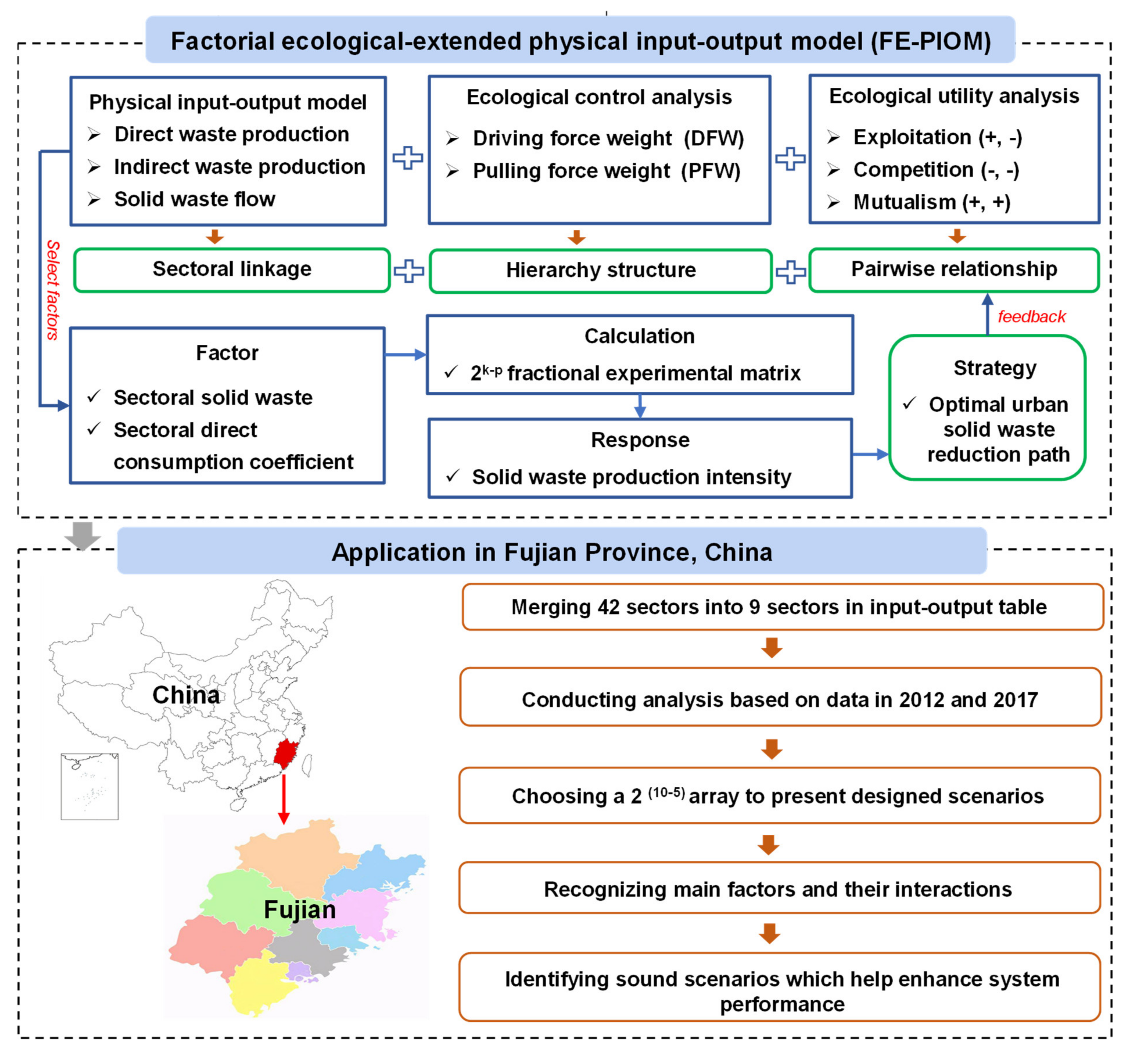
2. Materials and Methods

2.1. Physical Input-Output Model

The PIOM originates from the monetary IOM proposed by Leontief, and can reflect urban solid waste flows among sectors and investigate the multiple sectoral linkages [5,23]. The basic form of IOM can be presented as [27]:

$$x_i={\displaystyle \sum _{j=1}^n{z}_{ij}}+f{d}_i \mathrm{for} i=1 \mathrm{to} n$$

(1)

where x_i is the total output of sector i, z_ij is the amount of goods i that sector j consumes, and fd_i is the final demand of sector i. Solid waste intensity is then introduced to transform the monetary IOM into PIOM as follows [28,29]:

$$E+\mathsf{\epsilon }Z=\mathsf{\epsilon }X$$

(2)

$$\mathsf{\epsilon }=E{(X-Z)}^{-1}$$

(3)

$$F=diag(\epsilon )\ast Z$$

(4)

where E = [e_i]_1×n is the amount of sectoral solid waste; ε = [ε_i]_1×n is the solid waste intensity vector, ε_i is the embodied solid waste per unit of monetary value of sector i; Z = [z_ij]_n×n, z_ij is the amount of goods i that sector j consumes; X = [x_j]_1×n is the total economic output and F = [f_ij]_n×n is the solid waste flows among various sectors. By physical units, it is referred to mass units for presenting waste flows (e.g., Mg). Direct solid waste production equals the initial input of the monetary-physical input-output table, and the indirect solid waste production of each sector equals the sum of its column elements in the physical input-output table. For instance, sector i produces 1 Mg solid waste per unit product production, meaning 1 Mg is the amount of direct solid waste in sector i. Sector i sells product to sector j, implying that the 1 Mg solid waste is indirectly transferred to sector j (i.e., the amount of indirect solid waste in sector j is 1 Mg).

Then, the amount of sectoral indirect solid waste and sectoral total flows can be calculated based on Equations (5) and (6) [30]:

$$I{F}_j={\displaystyle \sum _{i=1}^n{f}_{ij}}$$

(5)

$$T_i={\displaystyle \sum _{j=1}^n{f}_{ij}}+e_i$$

(6)

where f_ij is the direct solid waste flowing from sector i to sector j; e_i is the amount of direct solid waste; IF_j is the amount of indirect sectoral solid waste and T_i is the total amount of waste. Taking all pathway flows with different lengths between two sectors into account, the dimensionless integral solid waste flow intensity matrix (N) can be obtained through:

$$g_{ij}=f_{ij}/T_i$$

(7)

$$N={(G)}^0+{(G)}^1+{(G)}^2+\dots {(G)}^{\infty }={(I-G)}^{-1}$$

(8)

where g_ij is the dimensionless input-oriented intercomponent flow from sector i to sector j; Gⁿ is the dimensionless integral flow intensity matrix with n path length and I(n×n) is the identity matrix.

2.2. Ecological Network Analysis

The dependence and control degrees of one sector to other sectors can present the system’s ecological hierarchy structure. The dependence degree means the ability of one sector receives urban solid waste from other sectors, while the control degree denotes the ability of one sector delivers urban solid waste to other sectors. The sum of all sectors’ dependence (or control) degrees is equal to 1. To reflect how the variations in solid waste flow of a sector influence the USWS’s ecological hierarchy structure, indexes (i.e., pulling force weight and driving force weight) in the ecological control analysis method are used to detect the sectoral dependence and control degrees as follows [31]:

$$Y=diag(T)\ast N$$

(9)

$$ID=Y-D=y_{ij}-f_{ij}$$

(10)

$$w_i={\displaystyle \sum _{j=1}^n{y}_{ij}^{}}/{\displaystyle \sum _{i=1}^n{\displaystyle \sum _{j=1}^n{y}_{ij}^{}}}$$

(11)

$$w_j={\displaystyle \sum _{i=1}^n{y}_{ij}^{}}/{\displaystyle \sum _{i=1}^n{\displaystyle \sum _{j=1}^n{y}_{ij}^{}}}$$

(12)

where Y is the sectoral contribution weight, y_ij is the integral flow from sector i to j, ID is the indirect flows of solid waste of sectors, w_j is the pulling force weight (PFW) of sector j, indicating the ability of sectors j receives solid waste from other sectors and w_i is the driving force weight (DFW) of sector i, meaning the ability of sector i delivers solid waste to other sectors. The difference between PFW and DFW indicates the role one sector plays in the waste flow chain.

Ecological utility analysis can be utilized to reveal the interconnection among various sectors in the USWS. The dimensionless direct utility matrix D examines the mutual benefit, and the integral utility intensity matrix U contains all solid waste interflows pathway. D and U can be calculated based on Equations (13) and (14) [32,33]:

$$D=[d_{ij}]=(f_{ij}-f_{ji})/T_i$$

(13)

$$U={(D)}^0+{(D)}^1+{(D)}^2+\dots {(D)}^{\infty }={(I-D)}^{-1}$$

(14)

Transforming U to sign(U) (including signU(+) and signU(−)) judges the integral ecological relationships between pairwise sectors. Relationships include: (i) exploitation (+, −) means sector i exploits j, indicating sector i receive wastes from j (the same applies to (−, +)); (ii) competition (−, −) means the relationship is harmful to both sectors; (iii) mutualism (+, +) means the relationship is beneficial to both sectors; (iv) neutralized (0, 0) means there is no impact on each other. Three indexes are employed to assess the comprehensive properties of the USWS:

$$SI={\displaystyle \sum _{i=1}^n{\displaystyle \sum _{j=1}^n{u}_{ij}}}$$

(15)

$$MI=\mathrm{sign}U(+)/\mathrm{sign}U(-)$$

(16)

$$R=\frac{N(+,+)+N(-,-)}{N}$$

(17)

where signU(+) and signU(−) are the number of positive and negative signs in U; N(+, +) and N(−, −) are the amounts of mutualism and competition relationships and N is the total number of all relationships. Synergism index (SI) and mutualism index (MI) assess fitness and symbiosis of the USWS [34]. When MI > 1 and SI > 0, the USWS is mutualistic. Otherwise, the USWS requires to be modified.

2.3. Fractional Factorial Analysis

The USWS involves a number of economic sectors. These sectors’ solid waste production may be interrelated to each other, increasing the complexity of the decision-making process. Fractional factorial analysis (FFA) can be employed to recognize the main factors and detect their interactions on the response variables of the USWS. Sectoral solid waste production (e_i in E) and sectoral direct consumption coefficient (a_ij = z_ij/x_j) can be chosen as factors, which are divided into multiple levels. Solid waste production intensity (abbreviated as SPI) can be selected as the response when SPI = direct solid waste production (Mg)/gross domestic product (10⁴ RMB¥ = 1542 USD). Using a fractional factorial analysis can screen main e_i and a_ij as well as quantify their interactions with reduced experimental cost. Researchers select an appropriate experimental matrix based on the number of e_i and a_ij [35]. A set of SPI values are gained by running the EIOM based on the matrix. Fractional factorial analysis quantifies the sensitivity of SPI to important factors and their combinations through addressing the curve traits of SPI when factors change at various levels. The quadratic sum for single factor and two-factor combinations are presented as follows [36,37]:

$$S{S}_A={{\displaystyle \sum _{i=1}^I\left({\displaystyle \sum _{j=1}^J{\displaystyle \sum _{k=1}^K{Y}_{ijk}}}\right)}}^2/JK-{\left({\displaystyle \sum _{i=1}^I{\displaystyle \sum _{j=1}^J{\displaystyle \sum _{k=1}^K{Y}_{ijk}}}}\right)}^2/IJK$$

(18)

$$S{S}_B={{\displaystyle \sum _{j=1}^J\left({\displaystyle \sum _{i=1}^I{\displaystyle \sum _{k=1}^K{Y}_{ijk}}}\right)}}^2/IK-{\left({\displaystyle \sum _{i=1}^I{\displaystyle \sum _{j=1}^J{\displaystyle \sum _{k=1}^K{Y}_{ijk}}}}\right)}^2/IJK$$

(19)

$$S{S}_{A\times B}={\displaystyle \sum _{i=1}^I{{\displaystyle \sum _{j=1}^J\left({\displaystyle \sum _{k=1}^K{Y}_{ijk}}\right)}}^2}/K-{\left({\displaystyle \sum _{i=1}^I{\displaystyle \sum _{j=1}^J{\displaystyle \sum _{k=1}^K{Y}_{ijk}}}}\right)}^2/IJK-S{S}_A-S{S}_B$$

(20)

$$S{S}_T={\displaystyle \sum _{i=1}^I{\displaystyle \sum _{j=1}^J{\displaystyle \sum _{k=1}^K{Y}^2{}_{ijk}}}}-{\left({\displaystyle \sum _{i=1}^I{\displaystyle \sum _{j=1}^J{\displaystyle \sum _{k=1}^K{Y}_{ijk}}}}\right)}^2/IJK$$

(21)

where I and J are the designed levels of factors A and B, respectively; y_ijk is the observed value in the K_th replication when A and B are at level I_th and J_th; SS_A, SS_B, and SS_A×B denote the square sum of A, B, and their combinations and SS_T is the total of squares. The contribution of each factor is calculated as the sum of its squares to the sum of the total squares.

3. Case Study

3.1. Study Area

Fujian Province lies between latitudes 23°33′ and 28°20′ N, and longitudes 115°50′ and 120°40′ E. It is an important economic development province with a land area of 121,400 km² located in the southeast coast of China. The total population of Fujian reached 41.54 million in 2020. It had a gross domestic product (GDP) of 0.677 trillion USD in 2020, occupying 4.3% of the whole country (the eighth place of all provinces in China). Over the past 40 years, the economic output of primary industry significantly decreased and the economic output of tertiary industry greatly increased. In 2017, the primary, secondary, and tertiary industries accounted for 6.9%, 47.7%, and 45.4% of the total GDP. The amount of direct urban solid waste reached 73.7 × 10⁶ Mg in 2017, while the corresponding comprehensive disposal-utilization rate was 66.9%. Compared with 2012, the amount of direct solid waste decreased 23.3% and disposal-utilization rate also decreased 22.7%. The decrease in direct waste production indicated that Fujian made some achievements in urban solid waste production reduction; however, the problem still concerns local managers.

3.2. Data Collection and Analysis

The 42-sector IOT of Fujian Province in 2012 and 2017 were extracted from Fujian Statistics Bureau. The 42 sectors were merged into nine sectors based on the Industrial Classification for Nation Economic Activities (GB/T 4754-2017), as described in

Table 1. Abbreviations of 9 sectors.

No.	Abbreviation	Sector
1	AGR	Agriculture, Forestry, Animal Husbandry and Fishery
2	MIN	Mining Industry
3	PM	Food, Wine, Drink, Tea Manufacturing and Tobacco Processing
		Textile Garments Products
		Timber Processing
		Paper Products
4	AM	Petroleum Processing, Coking and Nuclear Fuel Processing
		Chemical Products
		Nonmetal Minerals Products
		Smelting and Pressing of Metals
		Metal Products
		General and Special Equipment
		Transportation Equipment
		Electric Equipment and Machinery
		Computer, Communication and Other Electronic Equipment
		Instruments and Meters Machinery
		Others Manufacturing
5	ELE	Production and Supply of Electricity, Gas and Water
6	CON	Construction
7	TRA	Transportation, Storage and Postal Services
8	WHO	Wholesale, Retail and Accommodation
9	OTH	Other Social Services

.

Table 2. Merged economic input-output tables in 2012 and 2017 (10⁶ USD).

	Input	Intermediate Demand									Final Demand	Import	Import from Other Provinces	Total Output
Output		AGR	MIN	PM	AM	ELE	CON	TRA	WHO	OTH
In 2012
Intermediate input	AGR	3731	9	21,560	1276	1	770	83	3232	325	18,403	244	2590	46,555
	MIN	56	2253	772	19,410	4658	630	18	0	2	1311	4501	12,849	11,758
	PM	5793	189	80,049	7430	125	1237	486	3952	6523	110,528	12,345	4611	199,356
	AM	5387	2055	19,024	135,624	1677	42,888	8856	1359	7270	119,423	36,241	36,670	270,652
	ELE	570	653	4219	10,304	6444	692	1520	590	1844	3267	678	0	29,425
	CON	447	22	227	303	109	1237	615	14	467	117,306	36,221	0	84,652
	TRA	580	1040	5814	14,375	4348	6273	580	566	2232	12,003	8528	0	39,283
	WHO	717	324	6373	8237	1951	2413	1144	1647	7987	24,287	2348	0	52,733
	OTH	1770	817	5344	9181	2765	3031	9106	10,170	20,175	74,040	17,740	17	118,642
Added value		177,671	27,503	4397	55,975	64,512	7346	25,480	16,874	31,080	71,817	0	0	0
In 2017
Intermediate input	AGR	5635	6	34,154	1820	0	160	4866	692	786	27,473	9784	4707	61,102
	MIN	54	6112	13,257	24,993	3807	4367	7	0	152	141	24,102	16,587	12,201
	PM	7094	317	174,240	17,362	144	20,976	9144	8746	10,322	189,337	18,374	8410	410,896
	AM	7768	534	43,473	207,395	2215	30,917	13,514	732	7617	157,184	78,588	31,481	361,282
	ELE	571	439	4899	3574	18,867	680	4220	460	5870	1961	0	426	41,113
	CON	627	25	1182	982	723	1331	1345	153	974	145,435	0	352	152,426
	TRA	1183	454	11,048	7535	954	44,847	8090	2085	7611	24,938	0	4428	104,318
	WHO	798	198	14,900	7825	2587	2726	5977	1422	8144	47,164	0	3858	87,883
	OTH	1853	354	10,851	8040	2559	4505	14,481	23,786	56,404	118,745	32	11,611	229,935
Added value		229,443	35,518	3762	102,892	81,757	9257	41,917	42,675	49,807	132,055	0	0	0

lists the merged economic input-output tables in 2012 and 2017. The data of urban solid waste was obtained from Fujian Statistical Yearbook, related official website and literature [38,39]. A two-level fractional factorial analysis was adopted for designing a set of scenarios. Five sectoral solid waste production (e_i) and five sectoral direct consumption coefficients (a_ij) were selected as deigned factors, with each divided into low (L) and high (H) levels. According to the number of factors, a 2 ⁽¹⁰⁻⁵⁾ orthogonal array was chosen to present the experimental scenarios. Thirty-two SPI values were obtained through repeatedly running the model. The square sum of individual factor and factor combinations was calculated.

Figure 1 summarizes the formulation and application of the FE-PIOM model. The first step is to merge a large number of sectors into a small number of sectors in input-output table and transform the monetary input-output model into physical input-output model to describe sectoral linkages; calculate the driving force weight and pulling force weight to detect ecological hierarchy structure and then figure out the exploitation, competition, and mutualism to calculate ecological pairwise relationships. The second step is to select a set of proper factors, choose fractional experimental matrix, repeat the first step according to the matrix, recognize main factors and their interactions and identify a sound strategy.

4. Results and Discussion

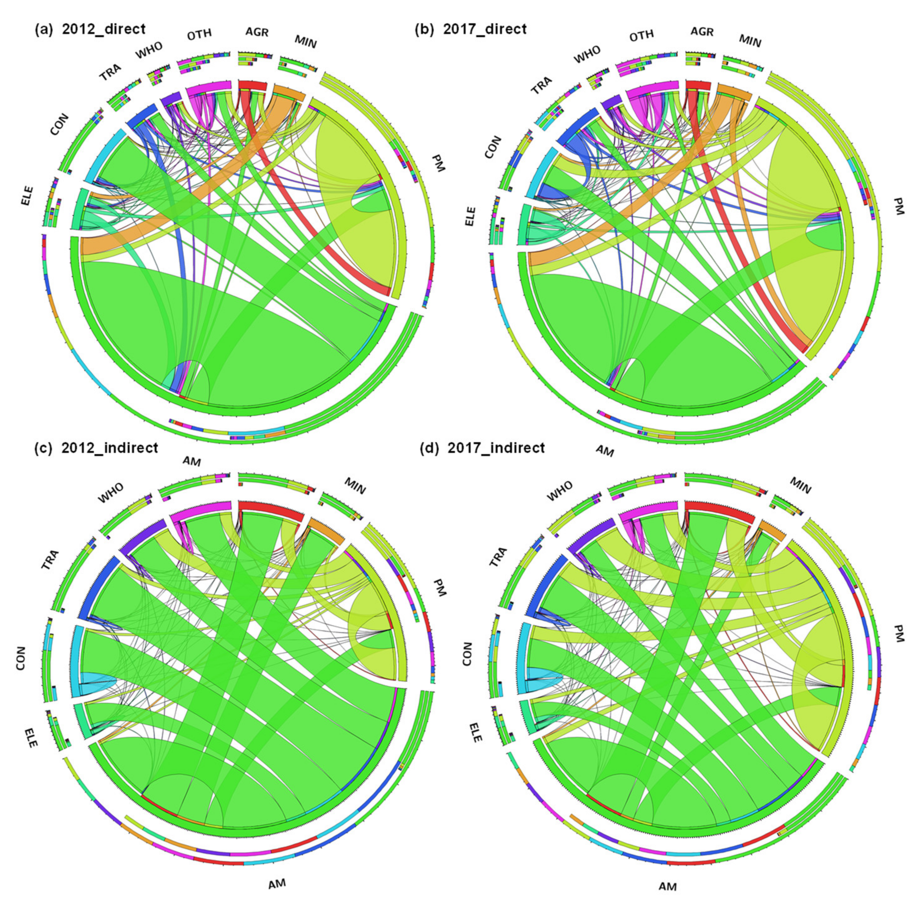
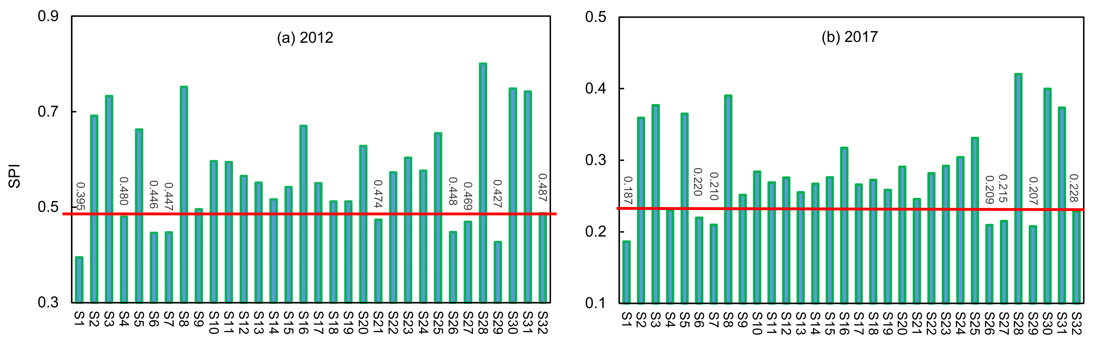
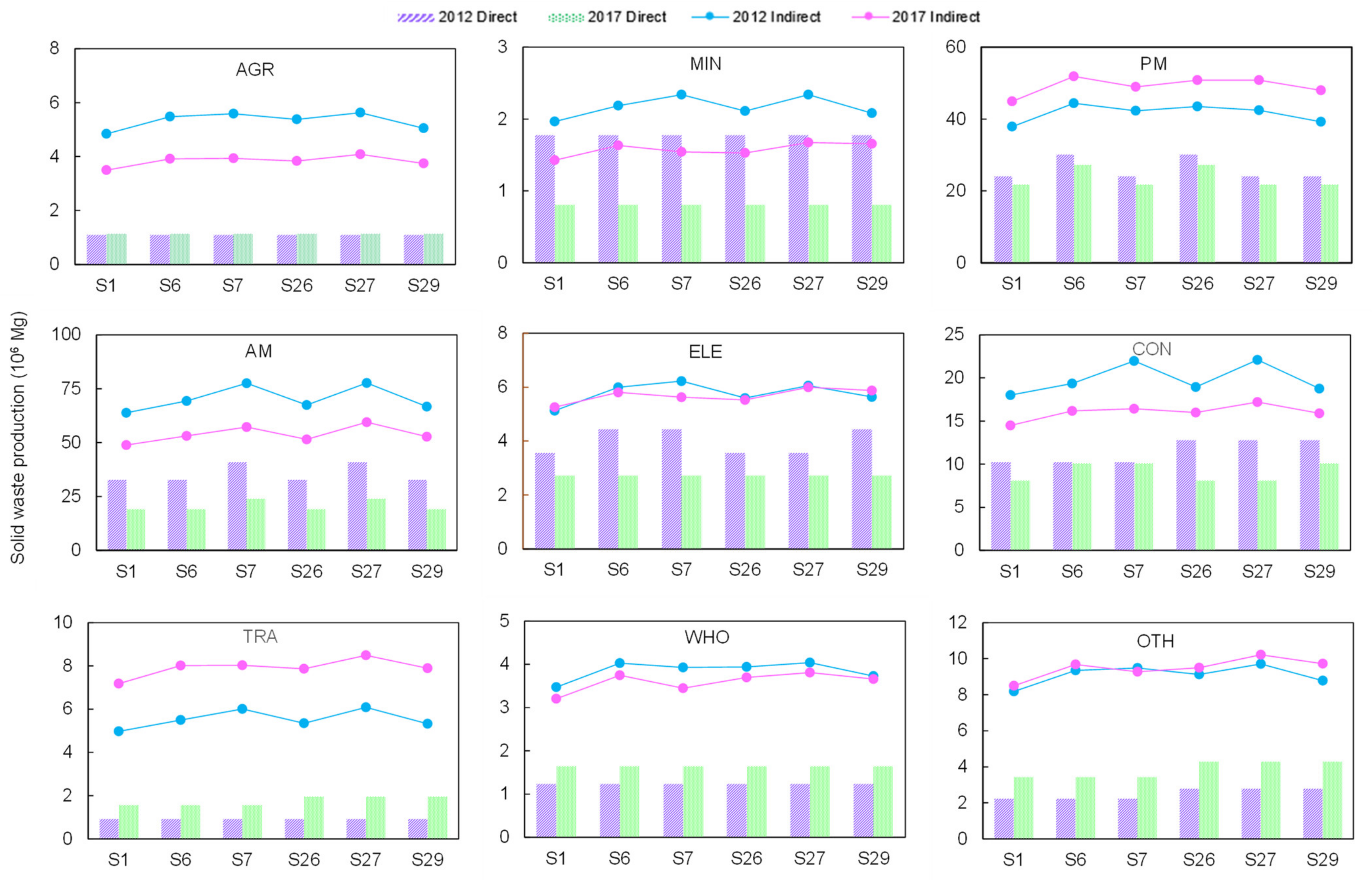
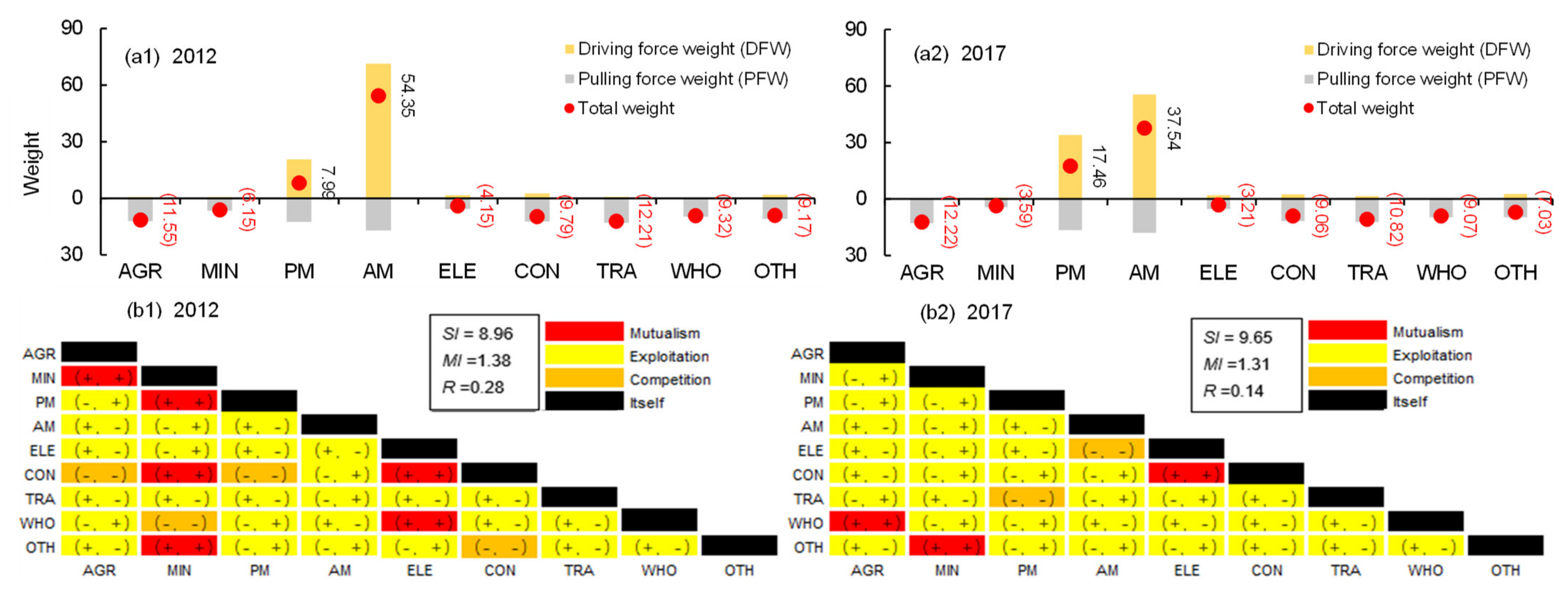
4.1. Status in 2012 and 2017

Table 3. Results gained from physical input-output table in Fujian in 2012 and 2017.

Sector	Sectoral Direct Solid Waste Production (106 Mg)	Sectoral Indirect Solid Waste Production (106 Mg)	Total Solid Waste Production Coefficient (10−6 Mg/USD)	Final Demand Production (106 Mg)	Export (106 Mg)	Import (106 Mg)	Net Import (106 Mg)
In 2012
AGR	1.091	5.899	3.598	2.115	0.649	0.426	−0.223
MIN	1.776	2.295	8.296	0.125	0.329	6.007	5.678
PM	30.105	46.337	9.188	11.898	30.484	6.502	−23.982
AM	40.871	76.985	10.435	20.202	31.802	31.750	−0.052
ELE	4.444	5.991	8.498	1.109	0.050	0.240	0.191
CON	12.783	21.925	9.825	46.873	1.224	14.851	13.627
TRA	0.921	6.051	4.253	1.224	0.906	1.514	0.607
WHO	1.236	4.220	2.479	1.346	1.167	0.243	−0.924
OTH	2.781	9.950	2.571	7.277	0.668	1.905	1.237
In 2017
AGR	1.138	4.164	2.080	2.331	0.054	1.257	1.204
MIN	0.807	1.526	4.582	0.009	0.018	7.780	7.762
PM	27.185	53.466	4.703	9.887	27.277	5.257	−22.019
AM	23.903	58.004	5.433	20.911	14.725	24.954	10.229
ELE	2.720	5.639	4.872	0.387	0.012	0.087	0.075
CON	10.085	17.274	4.301	26.090	0.013	0.063	0.050
TRA	1.943	8.459	2.389	2.038	0.449	0.442	−0.007
WHO	1.637	3.836	1.492	2.438	0.499	0.240	−0.259
OTH	4.283	9.985	1.487	7.149	0.220	0.722	0.503

lists sectoral solid waste production, solid waste production coefficients, and export/import of solid waste in Fujian. The total waste production approached 275.66 × 10⁶ t in 2012, where the direct and indirect productions accounted for 34.82% and 65.18%, respectively. Total waste production decreased to 236.05 × 10⁶ t in 2017, with direct and indirect productions decreasing by 23.23% and 9.63%, respectively. The amount of indirect waste production was more than that of direct waste production, implying the significance of the indirect production flow calculation. In 2012, PM, AM, and CON were the dominant contributors, occupying 27.73, 42.75 and 12.59% of the total solid waste production. In 2017, the proportions of the three sectors’ production were 34.17, 34.50, and 11.59%, respectively. These results revealed that solid waste was mainly produced by primary manufacturing (PM) and advanced manufacturing (AM). In addition, PM was the biggest solid waste net exporter (23.982 × 10⁶ t in 2012 and 22.019 × 10⁶ t in 2017) and CON was the largest importer (13.627 × 10⁶ t in 2012 and 10.229 × 10⁶ t in 2017). Fujian highly relied on clothing, lithium cells, auto parts manufacturing and food processing, and large amounts of construction materials were purchased from other provinces. Therefore, a future reduction strategy should focus on cutting down waste from these sectors.

Figure 2 describes the direct and indirect solid waste flows among sectors in 2012 and 2017. Each sector has a specific color and the line between sectors indicates the direction of waste flows. The width of the line in each sector represents the amount of waste inflow and outflow. All direct waste flows are positive, while indirect waste flows have positive and negative values. A positive value means one sector receives waste from the other sector, whereas a negative value denotes one sector delivers waste to the other sector. It can be seen that direct waste mainly flowed to CON, while indirect waste flowed to all sectors. In Figure 2a,b, the largest contributor of direct waste flow was AM, which contributed 54.23% and 44.18 % of the total amount in 2012 and 2017, respectively. It contributed a large part of its direct waste flow to CON and PM (occupying 27.62% in 2012 and 23.67% in 2017) and itself (accounting for 60.50% in 2012 and 66.01% in 2017). In Figure 2c,d, AM was still the largest contributor of indirect waste flow, which contributed 73.29% and 57.62 % of the total amount in 2012 and 2017, respectively. The indirect waste of AM flowing to all other sectors was almost the same (occupying 20% to 30%). These results show the relationship of indirect waste flows is more complicate than that of direct flows.

Figure 3a displays the sectoral DFW (driving force weight) and PFW (pulling force weight) in 2012 and 2017, representing the control and dependent degrees of a sector on the USWS. AM’s DFW and PFW were the highest; the values of DFW were 71.34% in 2012 and 55.43% in 2017; the values of PFW were 16.90% in 2012 and 17.89 % in 2017. These results indicate that AM was the biggest control sector and dependent sector that affected upstream sectors (basic industries that provide raw materials and primary products) and downstream sectors (advanced industry that consumes products from upstream). The sectoral total weight equals the difference between sectoral DFW and sectoral PFW. The sector was a controller in the system when DFW was greater than PFW, whereas the sector was a dependent sector in the system when DFW was smaller than PFW. Thus, AM finally acted as a controller, since its DFW was greater than PFW (Sectoral total weight = DFW−PFW > 0). It was obvious that AM and PM were dominant sectors that controlled the other producers, while the seven sectors (i.e., AGR, MIN, ELE, CON, TRA, WHO, and OTH) depended on the other sectors’ product supply. In 2017, the total weight of AM and PM decreased by 7.34% compared with 2012 due to reduced economic production scales. Generally, the ecological hierarchy structure was not healthy due to the high sectoral total weight value of AM. Carrying out reduction measures from the production side (especially from AM) could be helpful for adjusting hierarchy structure of the USWS.

Figure 3b shows the sectoral pairwise relationships related to solid waste production in 2012 and 2017, with a total of 45 pairs of relationships in each year. Exploitation relationships contributed 54.77% and 68.89% to all pairs of relationships in 2012 and 2017. The proportions of mutualism relationships were 13.33% in 2012 and 6.67% in 2017. High value of SI (i.e., SI = 8.96 > 0 in 2012, SI = 9.65 > 0 in 2017) indicated the synergistic effect of the USWS. A high value of MI (i.e., MI = 1.38 > 1 in 2012, MI = 1.31 > 1 in 2017) showed that the USWS was mutualistic. Results of sectoral pairwise relationships were acceptable for decision makers. However, the number of mutualism relationships in 2017 was less than that in 2012. In order to make the USWS more beneficial, exploitation relationships needed to be transformed to mutualism relationships, as much as possible, through adjusting strategies. It was also found that the production structure of Fujian had little changes.

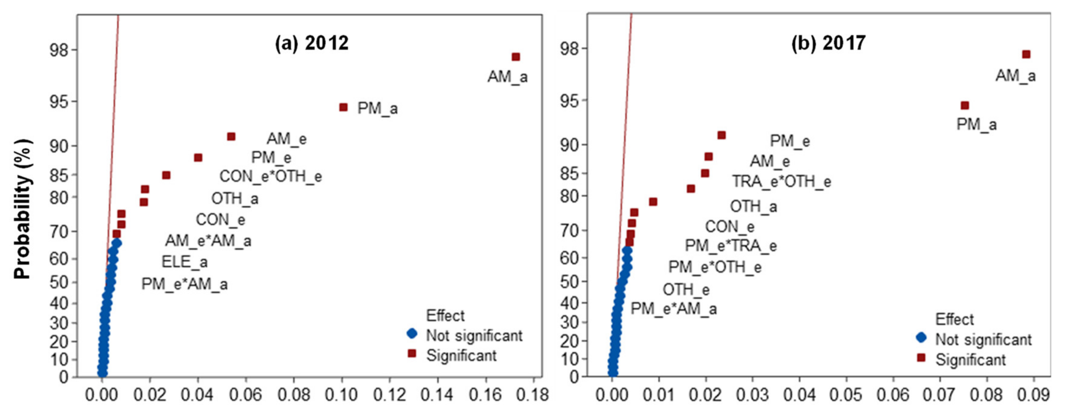
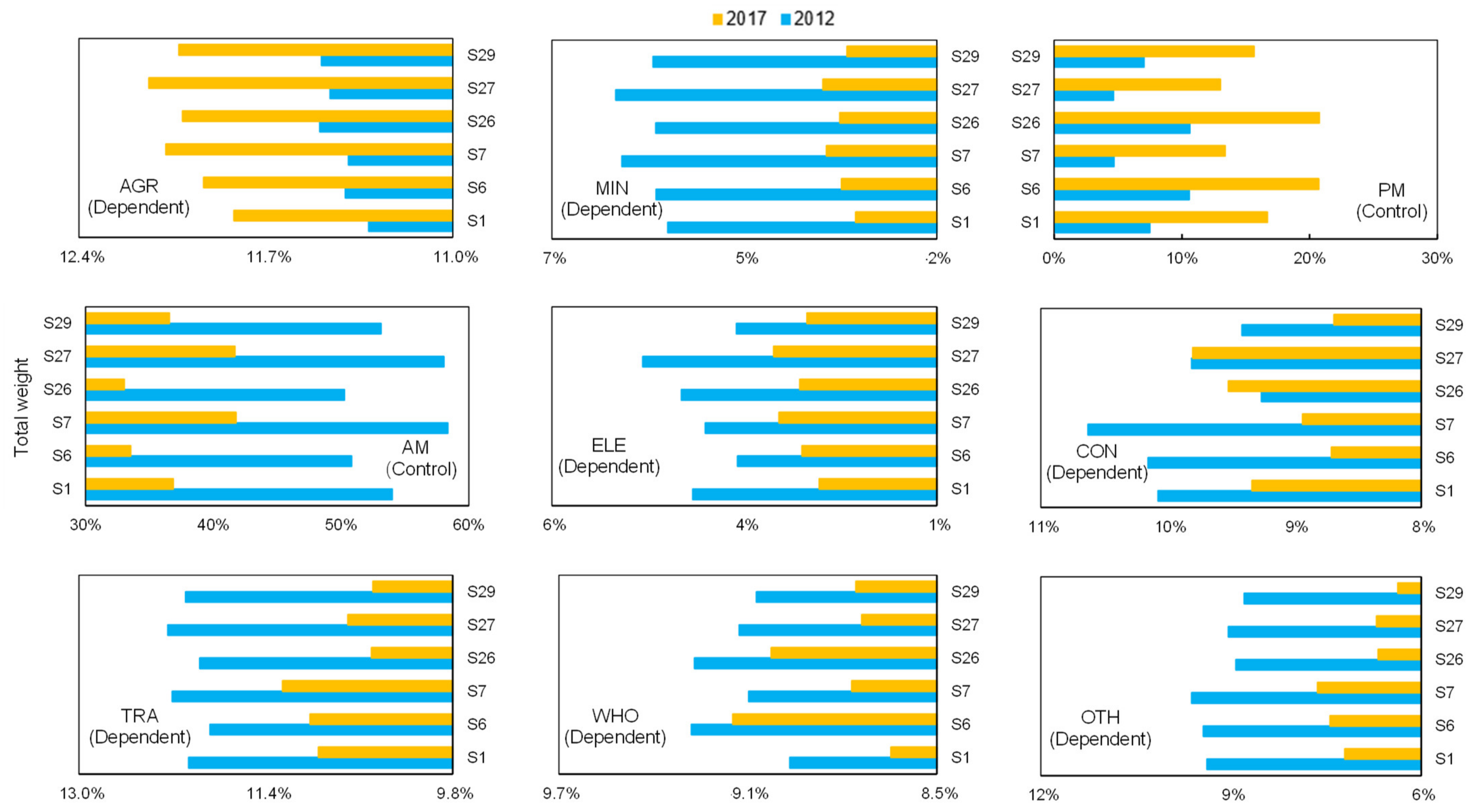
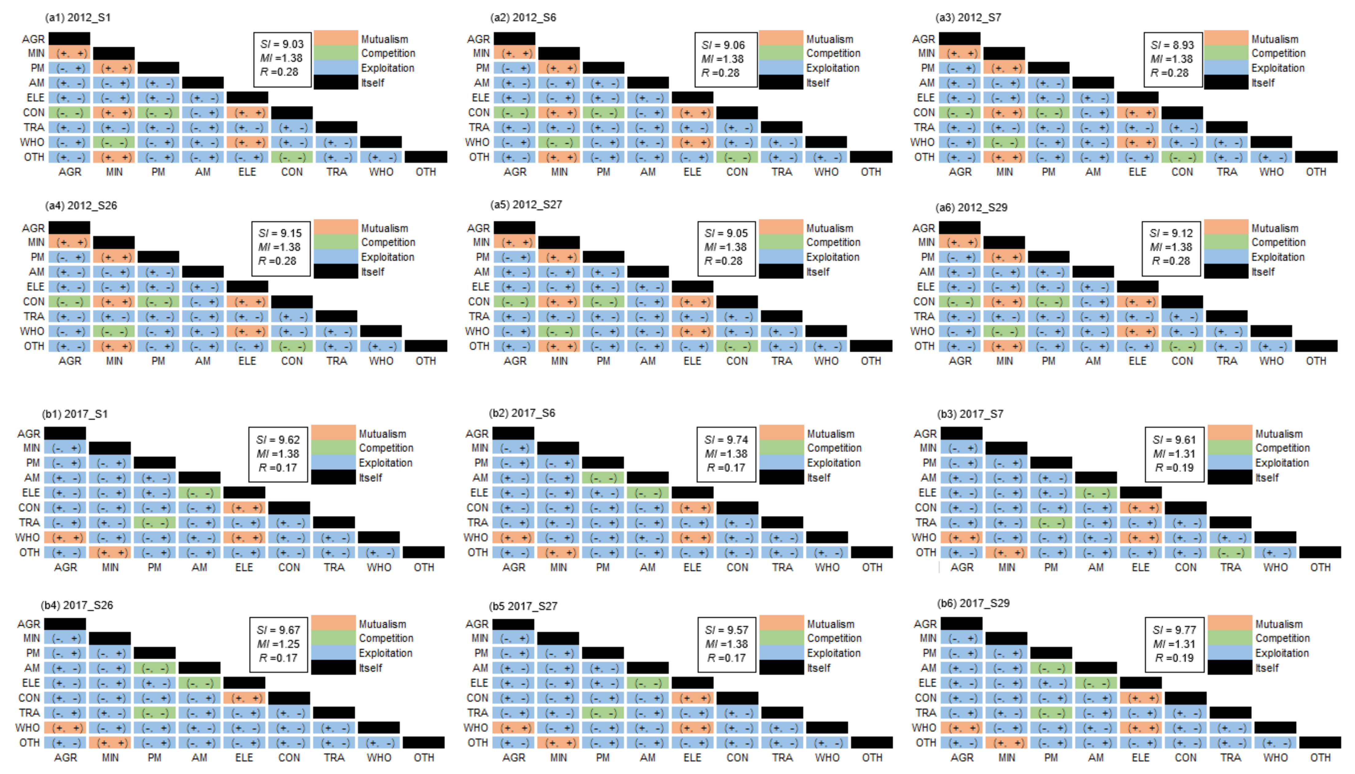
4.2. Identification of Key Factors

Based on the former status analysis, the effects of different sectoral solid waste production coefficients and sectoral direct consumption coefficients on USWS performance can be quantified. The designed factors, and corresponding experimental scenarios, are presented in

Table A2. Designed Scenarios.

Scenario	PM_e	AM_e	ELE_e (in 2012)	CON_e (in 2012)	OTH_e	PM_a	AM_a	ELE_a (in 2012)	CON_a (in 2012)	OTH_a
			CON_e (in 2017)	TRA_e (in 2017)				CON_a (in 2017)	TRA_a (in 2017)
1	L	L	L	L	L	H	H	H	H	H
2	H	L	L	L	L	L	L	L	L	H
3	L	H	L	L	L	L	L	L	H	L
4	H	H	L	L	L	H	H	H	L	L
5	L	L	H	L	L	L	L	H	L	L
6	H	L	H	L	L	H	H	L	H	L
7	L	H	H	L	L	H	H	L	L	H
8	H	H	H	L	L	L	L	H	H	H
9	L	L	L	H	L	L	H	L	L	L
10	H	L	L	H	L	H	L	H	H	L
11	L	H	L	H	L	H	L	H	L	H
12	H	H	L	H	L	L	H	L	H	H
13	L	L	H	H	L	H	L	L	H	H
14	H	L	H	H	L	L	H	H	L	H
15	L	H	H	H	L	L	H	H	H	L
16	H	H	H	H	L	H	L	L	L	L
17	L	L	L	L	H	H	L	L	L	L
18	H	L	L	L	H	L	H	H	H	L
19	L	H	L	L	H	L	H	H	L	H
20	H	H	L	L	H	H	L	L	H	H
21	L	L	H	L	H	L	H	L	H	H
22	H	L	H	L	H	H	L	H	L	H
23	L	H	H	L	H	H	L	H	H	L
24	H	H	H	L	H	L	H	L	L	L
25	L	L	L	H	H	L	L	H	H	H
26	H	L	L	H	H	H	H	L	L	H
27	L	H	L	H	H	H	H	L	H	L
28	H	H	L	H	H	L	L	H	L	L
29	L	L	H	H	H	H	H	H	L	L
30	H	L	H	H	H	L	L	L	H	L
31	L	H	H	H	H	L	L	L	L	H
32	H	H	H	H	H	H	H	H	H	H

. Figure 4 presents half-normal plots of the standardized effects. The further a factor lies away from the red line, the corresponding effect is more obvious. The significant factors that affected the SPI were AM_a, PM_a, AM_e and PM_e. The most important factor causing solid waste pollution in Fujian Province was AM_a, which contributed 64.71% in 2012 and 51.14% in 2017, followed by PM_a accounting for 22.01% and 37.04%. SPI was sensitive to the changes in sectoral direct consumption coefficients of AM and PM. These results implied that unit GDP solid waste production of AM and PM were higher than in other sectors. The contributions of AM_a decreased and PM_a increased in 2017, indicating that the Fujian Province gradually focused on the economic development of PM.

Figure 5 shows the effect plots of significant factors, which described the single and joint effects of the imperative factors on SPI. In Figure 5(a1,b1), results indicate that PM_a, AM_a, ELE_a and OTH_a had negative effects on SPIm, while other factors had positive effects on SPI. For example, in 2012, the average value of SPI was 0.632 under L level of PM_a and 0.533 under H level of PM_a. To reduce the SPI of USWS, the increment of factors that had negative effects, and the decrement of factors that had positive effects, might be helpful. In terms of joint effects presented in Figure 5(a2,b2), the most significant interactions between two sectors were CON_e*OTH_e in 2012 (contributed 1.53%) and TRA_e*OTH_e in 2017 (contributed 2.53%). The two crossed lines denote that the effect of another factor changes when one factor is at different levels. These demonstrated that control of the economic products of social service sectors (e.g., public infrastructure management sub-sector, culture, sports and entertainment sub-sector) can help reduce the SPI, even if the amounts of solid waste production of CON and TRA increased.

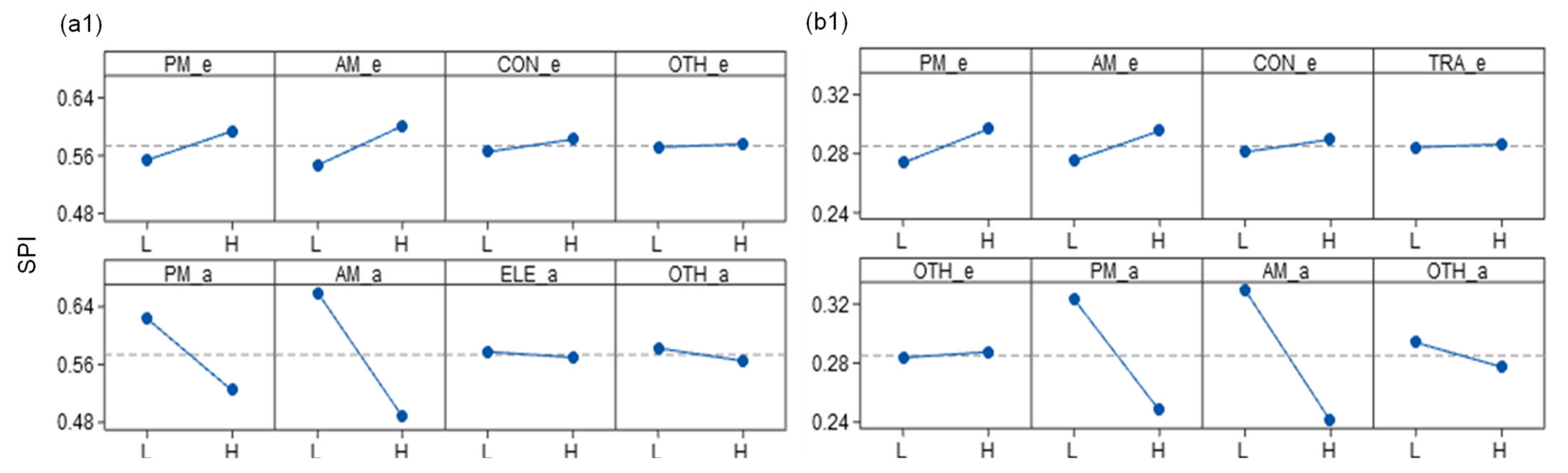
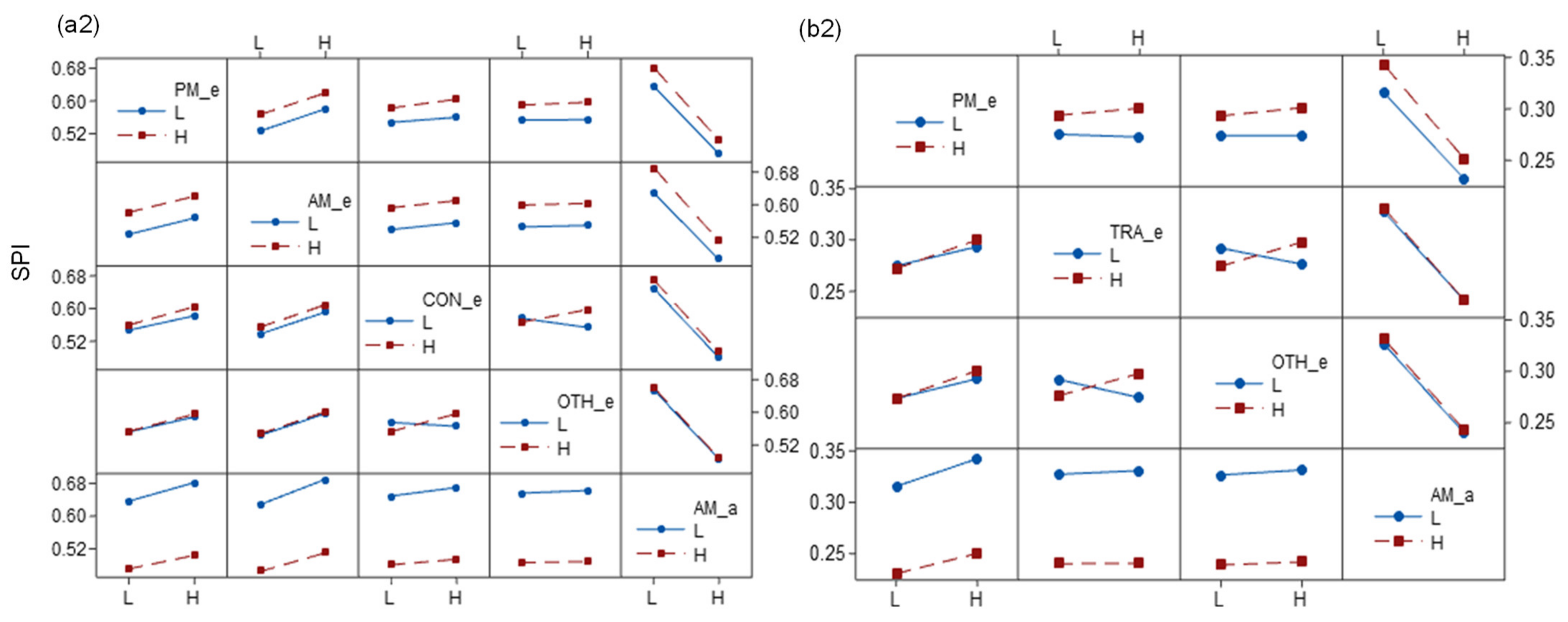
4.3. Adjustment of USWS

Figure 6 presents the values of solid waste production intensity (SPI) under 32 scenarios, showing the value of SPI was volatile. The SPI approached 0.487 (under S32) in 2012 and reached 0.228 (under S32) in 2017. The SPI decreased by 1.43% (under S4) to 18.89% (under S1) in 2012, and the SPI declined by 3.51% (under S6) to 17.98% (under S1) in 2017. Under S1, the strictest direct solid waste reduction policy was implemented in all sectors, while the sectoral direct consumption coefficients were maintained at high levels. Under S4 and S6, the loose direct solid waste reduction policy was implemented to PM, while the sectoral direct consumption coefficients of PM and AM were maintained at high levels. This implies that conducting strict environmental policy on AM and PM, as well as reducing the commodity consumption of CON, TRA, and OTH from other sectors (e.g., improve material usage efficiency and develop advanced material) would be useful for reducing SPI of the USWS.

Figure 7, Figure 8 and Figure 9 describe results of sectoral solid waste production and ecological network analysis under six scenarios in 2012 and 2017. Corresponding SPI values were lower than the actual values. In Figure 7, results showed that the amounts of solid waste production decreased by 3.82% (under S27) to 17.95% (under S1) in 2012 and decreased by 3.39% (under S27) to 16.30% (under S1) in 2017. The reduction of AM solid waste production was the highest among all sectors. In 2012, the amount decreased 34.438 × 10⁶ t (under S27) to 49.834 × 10⁶ t (under S1); in 2017, the amount reduced 1.511 × 10⁶ t (under S27) to 13.885 × 10⁶ t (under S1). These results reveal that the selected scenarios can effectively reduce solid waste production. In Figure 8, results indicate that the total weights of all sectors changed with the varied scenarios, implying that the system hierarchy structure was sensitive to the variations in factors. In 2012, the total weight of PM and AM were in the range of 61.47% (under S1) and 63.71% (under S4), an increase of −0.87% to 1.37% compared with that under S32. In 2017, the total weight of PM and AM was in the range of 53.53% (under S1) and 54.24% (under S6), a decrease by 0.75% to 1.46% compared with that under S32. According to former descriptions in status analysis, it was desired that the total weight of PM and AM should decrease. These results indicate that the selected designed scenarios could help adjust the hierarchical structure of USWS. In Figure 9, results show that the number of mutualistic, competitive, and exploitation relationships had no obvious changes; other measurements needed to be detected.

5. Conclusions

A factorial ecological-extended physical input-output model (FE-PIOM) was developed for enhancing urban solid waste system (USWS) performance, which integrated techniques of physical input-output model (PIOM), ecological network analysis (ENA), and fractional factorial analysis (FFA). The FE-PIOM could effectively assess urban solid waste productions and embodied flow path, quantify single and joint effects of multiple factors, as well as provide sound urban solid waste reduction path. The developed FE-PIOM was employed to a real case study of Fujian, an important economic development province in China, for supporting the tradeoff between economic development and environmental protection.

The main findings are summarized as: (i) the amount of indirect waste production was higher than the direct waste production, with the indirect production occupying more than 60 to 70% of the total production (i.e., the sum of direct and indirect productions); (ii) the indirect waste flows were more complicated than those of direct flows; (iii) solid waste mainly was produced by primary manufacturing (PM) and advanced manufacturing (AM), accounting for 30% and 38% of the total production, respectively; (iv) AM was the biggest sector which controlled the other producers, while its control weight was too high (35 to 50% of the total weight); (v) the USWS was mutualistic due to SI > 0 and MI > 1; (vi) AM_a (i.e., direct consumption coefficient of AM) and PM_a (i.e., direct consumption coefficient of PM) were the most important factors which had negative effects on USWS solid waste production intensity (SPI), contributing 50–60% and 22–37% to standard effects; (vii) the interactions between CON_e*OTH_e (i.e., solid waste production of CON*solid waste production of OTH) and TRA_e*OTH_e were obvious; (viii) for enhancing USWS performance, reducing the commodity consumption of AM and PM from other sectors by 20% (e.g., improve material usage efficiency and develop advanced material), as well as decreasing economic activities of CON, TRA, and OTH by 20%, would be useful.

This is the first attempt to apply the FE-PIOM to a real-world case, and results can support decision makers to adjust related economic activity strategies for reducing urban solid waste production, improving ecological hierarchy structure and promoting ecological pairwise relationships. More efforts can be made in future work. This research used the input-output tables of 2012 and 2017 due to data limitation; meanwhile, the production structure of Fujian had little changes in previous years. Predicting future input-output tables (e.g., for the periods of 2021–2025, 2026–2030, and 2031–2035) using the RAS method could help plan an optimal urban solid waste reduction path. It is essential to integrate fuzzy/stochastic analysis methods into the FE-PIOM to cope with the inherent uncertainties existing in economic growth, industrial structure transition and solid waste reduction.

References

1. Batista, M.; Caiado, R.G.G.; Quelhas, O.L.G.; Lima, G.B.A.; Filho, W.L.; Yparraguirre, I.T.R. A framework for sustainable and integrated municipal solid waste management: Barriers and critical factors to developing countries. J. Clean. Prod. 2021, 312, 127516. [Google Scholar] [CrossRef]
2. Karagoz, S.; Deveci, M.; Simic, A.; Aydin, N.; Bolukbas, U. A novel intuitionistic fuzzy MCDM-based CODAS approach for locating an authorized dismantling center: A case study of Istanbul. Waste Manag. Res. 2020, 1–13. [Google Scholar] [CrossRef]
3. China Statistical Yearbook; National Bureau of Statistics Press: Beijing, China, 2020. (In Chinese)
4. Simic, V.; Karagoz, S.; Deveci, M.; Aydin, N. Picture fuzzy extension of the CODAS method for multi-criteria vehicle shredding facility location. Expert Syst. Appl. 2021, 175, 114644. [Google Scholar] [CrossRef]
5. Danilina, V.; Grigoriev, A. Information provision in environmental policy design. J. Environ. Inform. 2020, 36, 1–10. [Google Scholar] [CrossRef]
6. Xu, X.; Huang, G.; Liu, L.; He, C. A factorial environment-oriented input-output model for diagnosing urban air pollution. J. Clean. Prod. 2019, 237, 117731. [Google Scholar] [CrossRef]
7. Xing, L.; Dong, X.; Guan, J.; Qiao, X. Betweenness centrality for similarity weight network and its application to measuring industrial sectors’ pivotability on the global value chain. Phys. A Stat. Mech. Appl. 2018, 516, 19–36. [Google Scholar] [CrossRef]
8. Liang, S.; Qu, S.; Xu, M. Betweenness-based method to identify critical transmission sectors for supply chain environmental pressure mitigation. Environ. Sci. Technol. 2016, 50, 1330–1337. [Google Scholar] [CrossRef]
9. Leontief, W. Input-Output Economics; Oxford University Press: Oxford, UK, 1986. [Google Scholar]
10. Towa, E.; Zeller, V.; Achten, W.M.J. Input-output models and waste management analysis: A critical review. J. Clean. Prod. 2020, 249, 119359. [Google Scholar] [CrossRef]
11. Liang, S.; Zhang, T.Z. Comparing urban solid waste recycling from the viewpoint of urban metabolism based on physical input–output model: A case of Suzhou in China. Waste Manag. 2012, 32, 220–225. [Google Scholar] [CrossRef]
12. Wang, H.N.; Wang, X.E.; Song, J.N.; Wang, S.; Liu, X.Y. Uncovering regional energy and environmental benefits of urban waste utilization: A physical input-output analysis for a city case. J. Clean. Prod. 2018, 189, 922–932. [Google Scholar] [CrossRef]
13. Meyera, D.E.; Li, M.; Ingwersen, W.W. Analyzing economy-scale solid waste generation using the United States environmentally-extended input-output model. Resour. Conserv. Recycl. 2020, 157, 104795. [Google Scholar] [CrossRef]
14. Huang, Q.; Chen, G.W.; Wang, Y.F.; Xu, L.X.; Chen, W.Q. Identifying the socioeconomic drivers of solid waste recycling in China for the period 2005–2017. Sci. Total Environ. 2020, 725, 138137. [Google Scholar] [CrossRef]
15. Balogun, A.; Quan, S.; Pradhan, B.; Dano, U.; Yekeen, S. An improved flood susceptibility model for assessing the correlation of flood hazard and property prices using geospatial technology and fuzzy-ANP. J. Environ. Inform. 2021, 37, 1–10. [Google Scholar] [CrossRef]
16. Zhang, Y.; Li, Y.G.; Hubacek, K.; Tian, X.; Lu, Z.M. Analysis of CO2 transfer processes involved in global trade based on ecological network analysis. Appl. Energy 2019, 233–234, 576–583. [Google Scholar] [CrossRef]
17. Wang, S.; Fath, B.; Chen, B. Energy-water nexus under energy mix scenarios using input-output and ecological network analyses. Appl. Energy 2019, 232–234, 827–839. [Google Scholar] [CrossRef]
18. Wang, R. Ecological network analysis of China’s energy-related input from the supply side. J. Clean. Prod. 2020, 272, 122796. [Google Scholar] [CrossRef]
19. Zheng, H.M.; Li, A.M.; Meng, F.X.; Liu, G.Y.; Hu, Y.C.; Zhang, Y.; Casazza, M. Ecological network analysis of carbon emissions from four Chinese metropoles in multiscale economies. J. Clean. Prod. 2021, 279, 123226. [Google Scholar] [CrossRef]
20. Montoya, A.C.V.; Mazareli, R.C.S.; Delforno, T.P.; Centurion, V.B.; Oliveira, V.M.; Silva, E.L.; Varesche, M.B.A. Optimization of key factors affecting hydrogen production from coffee waste using factorial design and metagenomic analysis of the microbial community. Int. J. Hydrog. Energy 2020, 45, 4205–4222. [Google Scholar] [CrossRef]
21. Yang, Y.; Huang, T.T.; Shi, Y.Z.; Wendroth, O.; Liu, B.Y. Comparing the performance of an autoregressive state-space approach to the linear regression and artificial neural network for streamflow estimation. J. Environ. Inform. 2021, 37, 1–10. [Google Scholar] [CrossRef]
22. Liu, J.; Li, Y.P.; Huang, G.H.; Fu, H.Y.; Zhang, J.L.; Cheng, G.H. Identification of water quality management policy of watershed system with multiple uncertain interactions using a multi-level-factorial risk-inference-based possibilistic-probabilistic programming approach. Environ. Sci. Pollut. Res. 2017, 24, 14980–15000. [Google Scholar] [CrossRef]
23. Lagrandeur, J.; Croquer, S.; Poncet, S.; Sorin, M. A 2D numerical benchmark of an air Ranque-Hilsch vortex tube based on a fractional factorial design. Int. Commun. Heat Mass Transf. 2021, 125, 105310. [Google Scholar] [CrossRef]
24. Jiang, Y.; Zhang, Y.; Banks, C.; Heaven, S.; Longhurst, P. Investigation of the impact of trace elements on anaerobic volatile fatty acid degradation using a fractional factorial experimental design. Water Res. 2017, 125, 458–465. [Google Scholar] [CrossRef] [Green Version]
25. Gerrewey, T.V.; Ameloot, N.; Navarrete, O.; Vandecruys, M.; Perneel, M.; Boon, N.; Geelen, D. Microbial activity in peat-reduced plant growing media: Identifying influential growing medium constituents and physicochemical properties using fractional factorial design of experiments. J. Clean. Prod. 2020, 256, 120303. [Google Scholar] [CrossRef]
26. Li, S.; Zhao, T.Y.; Chu, C.Q.; Wang, J.Q.; Alam, M.S.; Tong, T. Lateral cyclic response sensitivity of rectangular bridge piers confined with UHPFRC tube using fractional factorial design. Eng. Struct. 2021, 235, 111883. [Google Scholar] [CrossRef]
27. Almazán-Gómez, M.A.; Duarte, R.; Langarita, R.; Sánchez-Chóliz, J. Effects of water re-allocation in the Ebro river basin: A multiregional input-output and geographical analysis. J. Environ. Manag. 2019, 241, 645–657. [Google Scholar] [CrossRef]
28. Shafiei, M.; Moosavirad, S.H.; Azimifard, A.; Biglari, S. Water consumption assessment in Asian chemical industries supply chains based on input-output analysis and one-way analysis of variance. Environ. Sci. Pollut. Res. 2020, 27, 12242–12255. [Google Scholar] [CrossRef]
29. Chen, B.; Yang, Q.; Zhou, S.L.; Li, J.S.; Chen, G.Q. Urban Economy’s Carbon flow through external trade: Spatial-temporal evolution for macao. Energy Policy 2017, 110, 69–78. [Google Scholar] [CrossRef]
30. He, C.Y.; Huang, G.H.; Liu, L.R.; Xu, X.L.; Li, Y.P. Evolution of virtual water metabolic network in developing regions: A case study of Guangdong province. Ecol. Indic. 2020, 108, 105750. [Google Scholar] [CrossRef]
31. Zhai, M.Y.; Huang, G.H.; Liu, L.R.; Su, S. Dynamic input-output analysis for energy metabolism system in the Province of Guangdong, China. J. Clean. Prod. 2018, 196, 747–762. [Google Scholar] [CrossRef]
32. Owen, A.; Scott, K.; Barrett, J. Identifying critical supply chains and final products: An input-output approach to exploring the energy-water-food nexus. Appl. Energy 2018, 210, 632–642. [Google Scholar] [CrossRef]
33. Fath, B.D.; Patten, B.C. Review of the foundations of network environ analysis. Ecosystems 1999, 2, 167–179. [Google Scholar] [CrossRef]
34. Xia, C.Y.; Chen, B. Urban land-carbon nexus based on ecological network analysis. Appl. Energy 2020, 276, 115465. [Google Scholar] [CrossRef]
35. Fang, D.L.; Chen, B. Ecological network analysis for a virtual water network. Environ. Sci. Technol. 2015, 49, 6722–6730. [Google Scholar] [CrossRef] [PubMed]
36. Norouzi-Ghazbi, S.; Akbarzadeh, A.; Akbarzadeh-T, M.R. Application of Taguchi design in system identification: A simple, generally applicable and powerful method. Measurement 2020, 151, 106879. [Google Scholar] [CrossRef]
37. Montgomery, D.C. Design and Analysis of Experiments; John Wiley & Sons: Hoboken, NJ, USA, 1976. [Google Scholar]
38. Statistical Yearbook of Fujian Province; Fujian Provincial Bureau of Statistics: Fuzhou, China, 2013. (In Chinese). Available online: https://www.chinayearbooks.com/fujian-statistical-yearbook.html (accessed on 2 June 2021).
39. Statistical Yearbook of Fujian Province; Fujian Provincial Bureau of Statistics: Fuzhou, China, 2018. (In Chinese). Available online: https://www.chinayearbooks.com/fujian-statistical-yearbook-2018.html (accessed on 2 June 2021).
Figure 1. The formulation and application of the FE-PIOM model.
Sustainability 13 08341 g001
Figure 2. Direct and indirect solid waste flows among sectors. (a) 2012_direct; (b) 2017_direct; (c) 2012_indirect; (d) 2017_indirect.
Sustainability 13 08341 g002
Figure 3. Ecological network analysis. (a1) sectoral DFW and PFW in 2012; (a2) sectoral DFW and PFW in 2017; (b1) sectoral pairwise relationships in 2012; (b2) sectoral pairwise relationships in 2017.
Sustainability 13 08341 g003
Figure 4. Half-normal plots of the standardized effects: (a) 2012; (b) 2017.
Sustainability 13 08341 g004
Figure 5. Effect plots of significant factors. (a1) main effect in 2012; (a2) joint effect in 2012; (b1) main effect in 2017; (b2) joint effect in 2017.
Sustainability 13 08341 g005aSustainability 13 08341 g005b
Figure 6. The values of solid waste production intensity (SPI) under 32 scenarios: (a) 2012; (b) 2017. (“S” means “Scenario).
Sustainability 13 08341 g006
Figure 7. Sectoral urban solid waste production under different scenarios.
Sustainability 13 08341 g007
Figure 8. Sectoral total weight under different scenarios.
Sustainability 13 08341 g008
Figure 9. Pairwise sectoral relationships under different scenarios. (a1) 2012_S1; (a2) 2012_S6; (a3) 2012_S7; (a4) 2012_S26; (a5) 2012_S27; (a6) 2012_S29; (b1) 2017_S1; (b2) 2017_S6; (b3) 2017_S7; (b4) 2017_S26; (b5) 2017_S27; (b6) 2017_S29.
Sustainability 13 08341 g009