
Residential Energy Consumer Occupancy Prediction Based on Support Vector Machine


Abstract
:1. Introduction
- Electricity consumption is used as the only feature for binary occupancy classification in SVM. This saves system costs since no additional sensors are deployed to collect other measurements on energy consumers. Additionally, the computational workload is reduced since fewer data need to be processed;
- A divide-and-average method to reduce the dimension of the data inputted to SVM, hence save computational time and cost. In this method, a high-dimension feature vector is divided into low-dimension vectors which are then summed up and averaged to attain the final feature vector for SVM;
- The proposed approach gives better performances compared to the existing result in the literature on the same dataset.
2. Background on SVM
3. Energy Consumer Occupancy Prediction
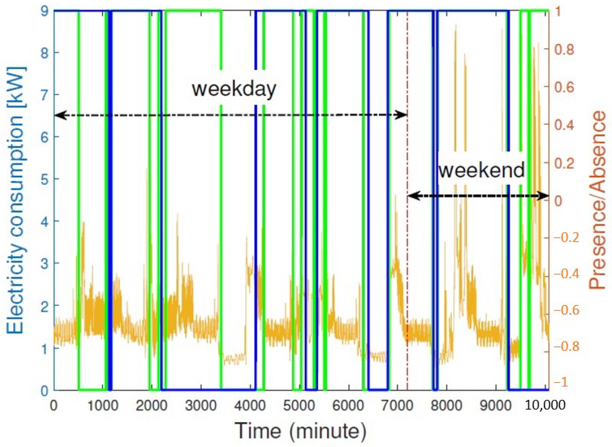
3.1. Electricity Consumption as a Learning Feature
3.2. Realistic Dataset
3.3. Prediction Results
- Confusion matrix: a matrix for binary classification whose first row composes of true positive (TP) and false negative (FN), while its second row composes of false positive (FP) and true negative (TN). Here, TP means the prediction of consumer presence and the home is occupied, FN means prediction of consumer absence and the home is occupied, FP means prediction of consumer presence and the home is not occupied, and TN means prediction of consumer absence and the home is not occupied;
- Accuracy
- Precision, or positive predictive value (PPV)
- True positive rate (TPR), or recall
- True negative rate (TNR)
- F1-score
- Matthews correlation coefficient (MCC)
- Balanced accuracy
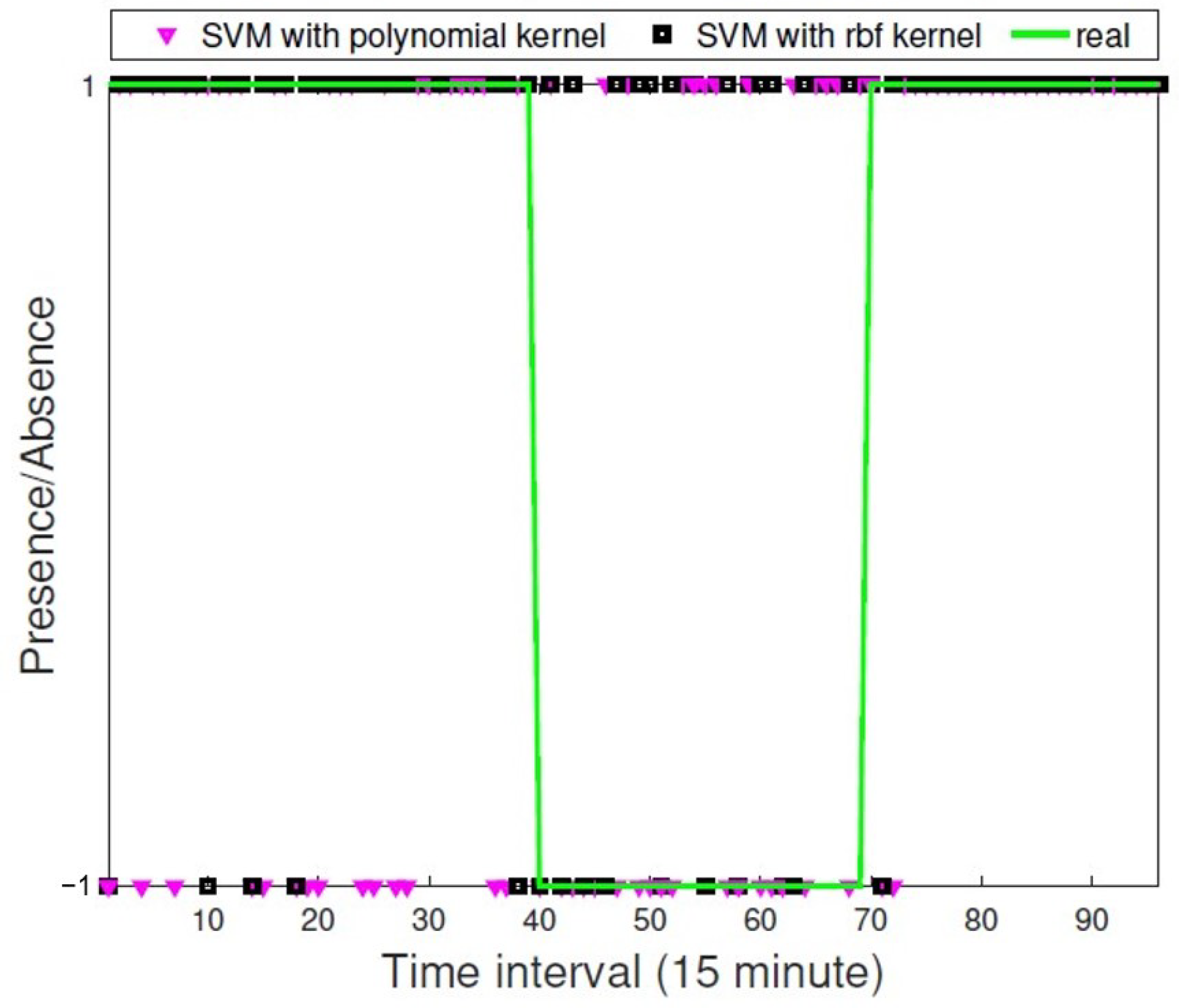
3.3.1. In Spring
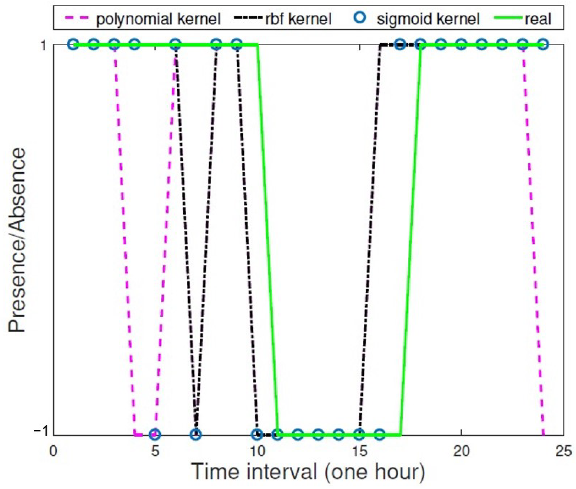
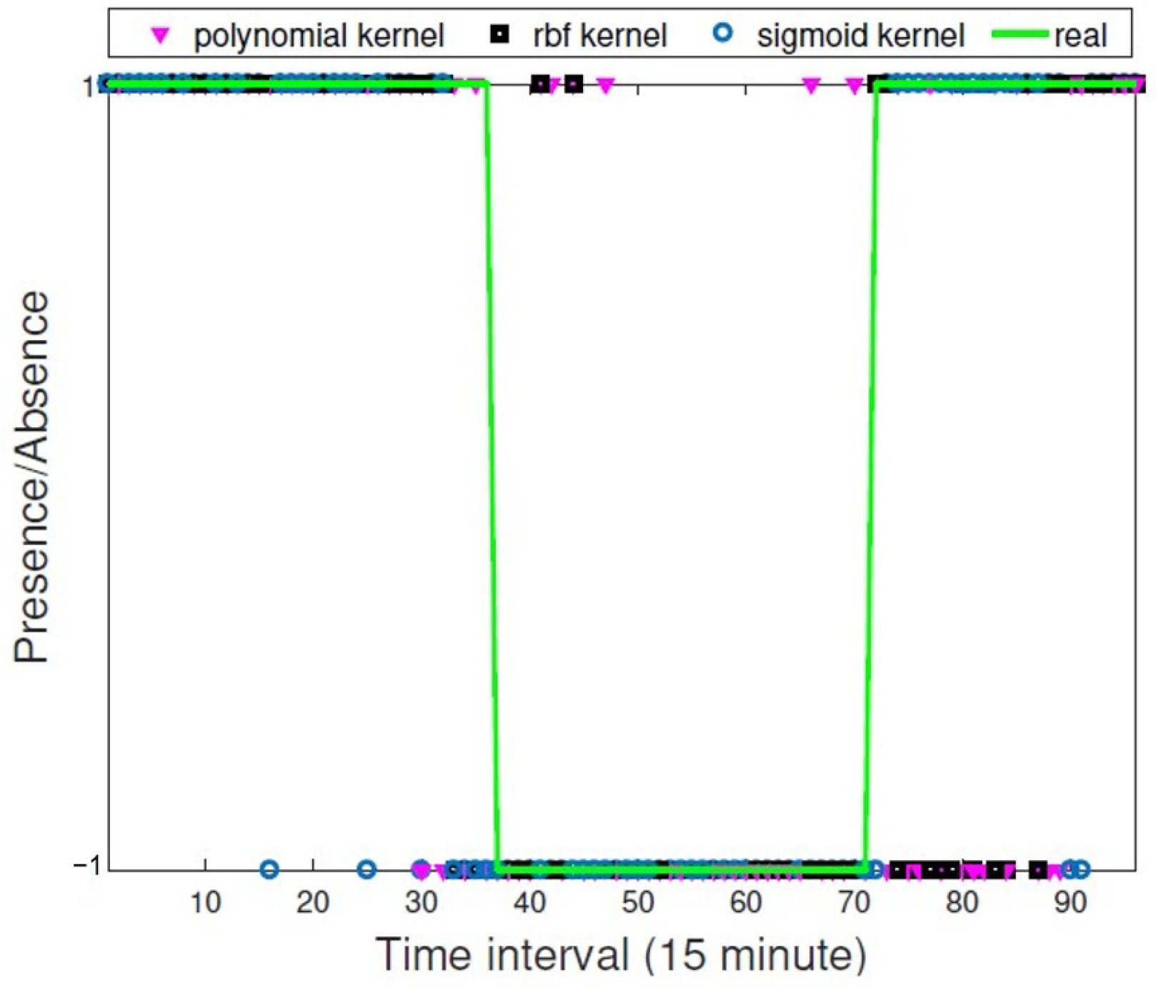
3.3.2. In Summer
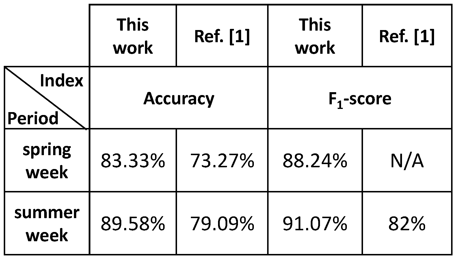
3.4. Comparison with Existing Results
4. Conclusions and Future Works
Funding
Acknowledgments
Conflicts of Interest
References
- Chen, D.; Barker, S.; Subbaswamy, A.; Irwin, D.; Shenoy, P. Non-Intrusive Occupancy Monitoring using Smart Meters. In Proceedings of the BuildSys’13: Proceedings of the 5th ACM Workshop on Embedded Systems for Energy-Efficient Buildings, Rome, Italy, 11–15 November 2013; pp. 1–8. [Google Scholar]
- Chaney, J.; Owens, E.H.; Peacock, A.D. An evidence based approach to determining residential occupancy and its role in demand response management. Energy Build. 2016, 125, 254–266. [Google Scholar] [CrossRef] [Green Version]
- Rueda, L.; Agbossou, K.; Cardenas, A.; Henao, N.; Kelouwani, S. A comprehensive review of approaches to building occupancy detection. Build. Environ. 2020, 180, 106966. [Google Scholar] [CrossRef]
- Dorokhova, M.; Ballif, C.; Wyrsch, N. Rule-based scheduling of air conditioning using occupancy forecasting. Energy AI 2020, 2, 100022. [Google Scholar] [CrossRef]
- Naylor, S.; Gillott, M.; Lau, T. A review of occupant-centric building control strategies to reduce building energy use. Renew. Sustain. Energy Rev. 2018, 96, 1–10. [Google Scholar] [CrossRef]
- Rana, A.; Perera, P.; Ruparathna, R.; Karunathilake, H.; Hewage, K.; Alam, M.S.; Sadiq, R. Occupant-based energy upgrades selection for Canadian residential buildings based on field energy data and calibrated simulations. J. Clean. Prod. 2020, 271, 122430. [Google Scholar] [CrossRef] [PubMed]
- Santiago, I.; Moreno-Munoz, A.; Quintero-Jiménez, P.; Garcia-Torres, F.; Gonzalez-Redondo, M. Electricity demand during pandemic times: The case of the COVID-19 in Spain. Energy Policy 2021, 148, 111964. [Google Scholar] [CrossRef] [PubMed]
- Abu-Rayash, A.; Dincer, I. Analysis of the electricity demand trends amidst the COVID-19 coronavirus pandemic. Energy Res. Soc. Sci. 2020, 68, 101682. [Google Scholar] [CrossRef] [PubMed]
- Madurai Elavarasan, R.; Shafiullah, G.; Raju, K.; Mudgal, V.; Arif, M.; Jamal, T.; Subramanian, S.; Sriraja Balaguru, V.; Reddy, K.; Subramaniam, U. COVID-19: Impact Analysis and Recommendations for Power Sector Operation. Appl. Energy 2020, 279, 115739. [Google Scholar] [CrossRef]
- Pecan Street. Shifting Energy Use Trends Due to COVID-19. 2020. Available online: https://www.pecanstreet.org/wp-content/uploads/2020/05/Covid-Webinar-May-2020-Slide-Deck-.pdf (accessed on 18 June 2021).
- New York Independent System Operator. Recent Impacts on Hourly Load Patterns. 2020. Available online: https://www.nyiso.com/-/covid-19-and-the-electric-grid-load-shifts-as-new-yorkers-respond-to-crisis (accessed on 18 June 2021).
- Zuraimi, M.; Pantazaras, A.; Chaturvedi, K.; Yang, J.; Tham, K.; Lee, S. Predicting occupancy counts using physical and statistical CO2-based modeling methodologies. Build. Environ. 2017, 123, 517–528. [Google Scholar] [CrossRef]
- Chidurala, V.; Li, Z. Occupancy Estimation Using Thermal Imaging Sensors and Machine Learning Algorithms. IEEE Sens. J. 2021, 21, 8627–8638. [Google Scholar] [CrossRef]
- Wang, C.; Jiang, J.; Roth, T.; Nguyen, C.; Liu, Y.; Lee, H. Integrated sensor data processing for occupancy detection in residential buildings. Energy Build. 2021, 237, 110810. [Google Scholar] [CrossRef]
- Sardianos, C.; Varlamis, I.; Chronis, C.; Dimitrakopoulos, G.; Himeur, Y.; Alsalemi, A.; Bensaali, F. A model for predicting room occupancy based on motion sensor data. In Proceedings of the 2020 IEEE International Conference on Informatics, IoT, and Enabling Technologies (ICIoT), Doha, Qatar, 2–5 February 2020; pp. 394–399. [Google Scholar]
- Jin, M.; Jia, R.; Spanos, C.J. Virtual Occupancy Sensing: Using Smart Meters to Indicate Your Presence. IEEE Trans. Mob. Comput. 2017, 16, 4490–4501. [Google Scholar] [CrossRef] [Green Version]
- Wei, Y.; Xia, L.; Pan, S.; Wu, J.; Zhang, X.; Han, M.; Zhang, W.; Xie, J.; Li, Q. Prediction of occupancy level and energy consumption in office building using blind system identification and neural networks. Appl. Energy 2019, 240, 276–294. [Google Scholar] [CrossRef]
- Ryu, S.H.; Moon, H.J. Development of an occupancy prediction model using indoor environmental data based on machine learning techniques. Build. Environ. 2016, 107, 1–9. [Google Scholar] [CrossRef]
- Feng, C.; Mehmani, A.; Zhang, J. Deep Learning-based Real-time Building Occupancy Detection Using AMI Data. IEEE Trans. Smart Grid 2020, 11, 4490–4501. [Google Scholar] [CrossRef]
- Himeur, Y.; Ghanem, K.; Alsalemi, A.; Bensaali, F.; Amira, A. Artificial intelligence based anomaly detection of energy consumption in buildings: A review, current trends and new perspectives. Appl. Energy 2021, 287, 116601. [Google Scholar] [CrossRef]
- Liu, C.; Akintayo, A.; Jiang, Z.; Henze, G.P.; Sarkar, S. Multivariate exploration of non-intrusive load monitoring via spatiotemporal pattern network. Appl. Energy 2018, 211, 1106–1122. [Google Scholar] [CrossRef]
- Iqbal, H.K.; Malik, F.H.; Muhammad, A.; Qureshi, M.A.; Abbasi, M.N.; Chishti, A.R. A critical review of state-of-the-art non-intrusive load monitoring datasets. Electr. Power Syst. Res. 2021, 192, 106921. [Google Scholar] [CrossRef]
- Fransson, V.; Bagge, H.; Johansson, D. A method to estimate absence in apartments based on domestic water use. Build. Environ. 2020, 180, 107023. [Google Scholar] [CrossRef]
- Cristianini, N.; Shawe-Taylor, J. An Introduction to Support Vector Machines and Other Kernel-Based Learning Methods; Cambridge University Press: Cambridge, UK, 2000. [Google Scholar] [CrossRef]
- Lin, H.T. A Study on Sigmoid Kernels for SVM and the Training of Non-PSD Kernels by SMO-Type Methods. 2005. Available online: https://home.work.caltech.edu/~htlin/publication/doc/tanh.pdf (accessed on 23 April 2021).
- Laboratory for Advanced System Software, University of Massachusetts Amherst, USA. NIOM Occupancy Dataset. 2017. Available online: http://traces.cs.umass.edu/index.php/Smart/Smart (accessed on 23 April 2021).


Publisher’s Note: MDPI stays neutral with regard to jurisdictional claims in published maps and institutional affiliations. |
© 2021 by the author. Licensee MDPI, Basel, Switzerland. This article is an open access article distributed under the terms and conditions of the Creative Commons Attribution (CC BY) license (https://creativecommons.org/licenses/by/4.0/).
Share and Cite
Nguyen, D.H. Residential Energy Consumer Occupancy Prediction Based on Support Vector Machine. Sustainability 2021, 13, 8321. https://doi.org/10.3390/su13158321
Nguyen DH. Residential Energy Consumer Occupancy Prediction Based on Support Vector Machine. Sustainability. 2021; 13(15):8321. https://doi.org/10.3390/su13158321
Chicago/Turabian StyleNguyen, Dinh Hoa. 2021. "Residential Energy Consumer Occupancy Prediction Based on Support Vector Machine" Sustainability 13, no. 15: 8321. https://doi.org/10.3390/su13158321
APA StyleNguyen, D. H. (2021). Residential Energy Consumer Occupancy Prediction Based on Support Vector Machine. Sustainability, 13(15), 8321. https://doi.org/10.3390/su13158321