Eco-Acoustic Assessment of an Urban Park by Statistical Analysis

Abstract

We investigated the statistical properties of the sounds recorded at a site located in the Parco Nord of Milan, Italy, characterized by wooded land rich in biodiversity and exposed to different sources and types of anthropogenic disturbances with the aim of deriving information on its environmental quality in terms of biophonic presence and athropic disturbance. A time series of eco-acosutic indices were determined for 616 audio files recorded from 30 April 2019 (5:00 p.m.) to 3 May 2019 (5:00 a.m.) with a 1-min duration followed by a 5-min pause (10 recordings per hour). In the present study, the following indices were computed: the Acoustic Complexity Index (ACI), Acoustic Diversity Index (ADI), Acoustic Evenness Index (AEI), Bio-acoustic Index (BI), Acoustic Entropy Index (H), Normalized Difference Soundscape Index (NSDI) and Dynamic Spectral Centroid (DSC). Cluster analysis performed on the corresponding time series yielded a dimensional reduction from seven down to three. The results show a clear separation of the eco-acoustic indices into two clusters, reflecting the different dynamics and diversity behaviour throughout the recordings. A post-processing aural survey was also performed, aiming at determining biophonic activities (mainly avian vocalization and other animals), the characteristics of technophonies sources (mainly road traffic noise and airplane fly-overs), human presence (voices and steps) and geophonies (rain and wind). The statistical analysis proved to be a robust tool due to the good matching obtained with the aural survey outcomes. The overall quality of the Parco Nord phonic activity was found to be low. Notwithstanding the presence of avian species, highlighted by the characteristic dawn chorus, both clusters revealed low “scores” of NDSI and DSC indices heavily influenced by road traffic sources. This study represents the first step toward the realization of maps of eco-acoustic indices for the long-term monitoring of fragile habitats.

1. Introduction

Eco-acoustics and bioacoustics encompass the study of environmental sounds and the sounds produced by or affecting living organisms. They have grown in importance as non-invasive techniques for ecological monitoring during the last decades. In particular, eco-acoustics investigates the soundscape, which can be defined as the collection of sounds that emanate from a landscape, composed of sounds from physical (geophony), biological (biophony) and anthropogenic (anthrophony or technophony) sources [1,2,3]. The basic idea behind eco-acoustics is that measurements of the acoustic ambience could potentially convey important information about an environment, such as species presence (bioindicators), environmental conditions and habitat quality [4].

Current environmental degradation, including climate change, habitat destruction, chemical pollution and anthropogenic noise, affect the environment and, consequently, natural populations. Although the sounds produced by human activity are part of the soundscape, noise can also be considered as a pollutant for the environment, potentially masking communication signals between living organisms or causing modifications in their population size, density and demography.

An exponential increase in the application of acoustic techniques has recently occurred in mainly terrestrial realms [5,6]. Passive acoustic monitoring (PAM) can help sampling and monitoring ecosystems, since it provides the unique opportunity to rapidly quantify and compare sound across habitats, space and time. Sounds play an important role in detecting the first signs of stress in animals, including from individual species, populations, communities, and landscapes. Environmental conditions, on which physical and chemical pollutants and climate change act, have direct effects on the presence of species and on their acoustic performance, which are the results of complex interactions between the energetic environment, the animal biomass and the structure of the social interactions.

PAM can be used to monitor terrestrial habitats [7,8], marine habitats [9,10], freshwater environments [11,12] and urban areas [13,14]. In marine and terrestrial habitats, sounds can fluctuate over different time scales creating peculiar soundscape signatures. A soundscape signature potentially distinguishes every habitat type, through the description of the collected sounds [8].

Indeed, PAM has several advantages compared to traditional methods (e.g., visual field observations, satellite remote sensing, netting and electrofishing for the aquatic settings). It is a non-invasive technique that minimizes disturbances to animal behaviour and environmental impacts [15]. Moreover, it allows collecting a great amount of data for long periods and furthermore, with the advent of autonomous and weather resistant recorders, measurements can be undertaken with reasonable efforts and costs [5,16]. Finally, PAM enables to access a greater range of habitats and has particularly strong potential in low visibility environments, such as dense forests or underwater, because sound propagation is not as strongly impacted by obstacles as other sensing methods, such as visual detection.

Several acoustic or eco-acoustic indices have been developed to assess the complexity and dynamics of soundscape and to act as proxies of species assemblage diversity measures to characterize environmental quality [7,15,17]. In general, a successful index must be: positively correlated with traditional species assemblage measurements in relevant frequency ranges; robust to changes in spectral resolution; and robust to the inclusion of natural and anthropogenic noise interference in the acoustic data set.

These indices are usually obtained through the post processing of sound frequencies and levels to extract specific characteristics of the sound and consequently of the soundscape. Among them, the most used are: the Acoustic Entropy Index (H), which reflects the evenness of a signal’s amplitude over time and across the full range of frequencies [15]; the Acoustic Richness (AR), which is based on H but weights the signal by its median amplitude to account for background noise and measures the acoustic richness of a community [7]; the Acoustic Complexity Index (ACI), which determines the modulation in intensity of a given recording over changing frequencies [17]; the Normalized Difference Soundscape Index (NDSI), which computes the ratio between human-generated and biological acoustic components to evaluate the disturbance on a landscape [18]; the Dynamic Spectral Centroid (DSC), based on the time-pattern of the gravity centre of a spectrum, which represents a measure of the spectral content of the soundscape [19]; and the Acoustic Diversity Index (ADI) [19], calculated by dividing the spectrogram into bins and taking the relative signal in each bin above a threshold.

The ADI is the result of the Shannon index, H, Ref. [20] applied to the spectrogram bins; similarly, the Acoustic Evenness Index (AEI) [19] is the result of the Gini index applied to the spectrogram bins [21].

The skill of these indices to capture different sound characteristics, suggests adopting an integrated approach to describe the complexity of urbanized natural environments, such as those found in medium–large urban parks. Here, the presence of biophonic activities is facing to anthropogenic noise sources, especially at the parks’ limiting areas. In this paper, we analyse the recordings taken at one site in the Parco Nord of Milan, Italy, with the aim of deriving an analysis method to establish an environmental quality tool and provide useful indications to improve the use of the park.

The analysis reported in previous works [14,22] showed how eco-acoustic indices behave in different background and biophonic activity conditions. The aim of those studies was to evaluate the potential of eco-acoustic indicators for the discrimination of habitats with different degrees of anthropogenic noises and with higher biophonic activities (e.g., sounds in medium–large urban parks as compared to pristine habitats using short audio recordings). Here, we assess the validity of a statistical approach for long audio recordings (more than 60 h) by comparing the results with aural surveys.

Soundscape characteristics can be described by different eco-acoustics indices, which tend to amplify and highlight sound/frequency-specific features. Patterns in data-recordings could, thus, be uncovered by unsupervised statistical analysis applied to such sound characteristic (eco-acoustic) time series. We chose to analyse the recordings taken at one site in the Parco Nord of Milan with the aim of deriving a new method of analysis to establish an environmental quality tool and provide useful indication to address the use of the park when applied to a larger area.

2. Material and Methods

In the first part of this section, we will describe the area of the study, the instrumentation used and the acquisition sequence. In the second part, we will illustrate the analysis methodology based on the calculation of the eco-acoustic indices and the statistical analysis. Eventually, we will describe the aural survey with all the categories of sounds considered for validation of the results.

2.1. Area of the Study

The studied area is a large peri-urban park in northern Milan (Parco Nord), characterized by wooded land rich in biodiversity and exposed to different sources and degrees of anthropogenic disturbances, such as road traffic noise and artificial light. The Parco Nord of Milan covers about 640 hectares in the north side of the city of Milan, rounded by an intensely urbanized area. About 250 hectares (40%) of this area are occupied by green spaces and trees, while the remainder is used for agricultural purposes and infrastructures. More in detail, the 250 hectares of greenery are divided between wooded areas (over 80 ha), meadows, shrubs, hedges and small stretches of water.

Among the tall trees, shrubs and ornamental plants, currently Parco Nord counts the presence of over 100 species, among which, 30% are indigenous. The study area in which the sound recordings were performed is located in the south part of Parco Nord, in a wooded parcel with a semi-natural structure with a herbaceous layer, a shrub layer and the presence of dead wood. There is a small artificial body of water (about 800 m${}^2$) near the edge of the wooded area. Visitors use this area mainly for walking or playing sports, as it is crossed by numerous paths, or for recreational activities. Thus, the site was chosen for its exposure to the variety and multitude of natural and anthropic sounds.

The audio files analysed in this study were recorded from 30 April (5 p.m.) to 3 May (5 a.m.) 2019 according to the schedule of 1 min recordings followed by 5 min pauses, leading to 10 recordings per hour (total recordings: 616). A Soundscape Explorer Terrestrial (SET) recorder unit was used for this analysis. This device is a sound and meteorological data recorder for terrestrial environments that provides real-time acoustic complexity index (ACI) computation.

It is equipped with two microphones, an electronic control board, a full set of meteorological sensors (for recording the pressure, temperature, relative humidity and ambient light) and a rechargeable lithium battery pack, all contained in a waterproof plastic case. One of the two microphones of the recorder targets low frequencies and acquires data in the sonic range (up to 24 kHz and sample rate 48 kHz), and the other microphone targets high frequencies and acquires data in the sonic and ultrasonic ranges (up to 96 kHz and sample rate 192 kHz).

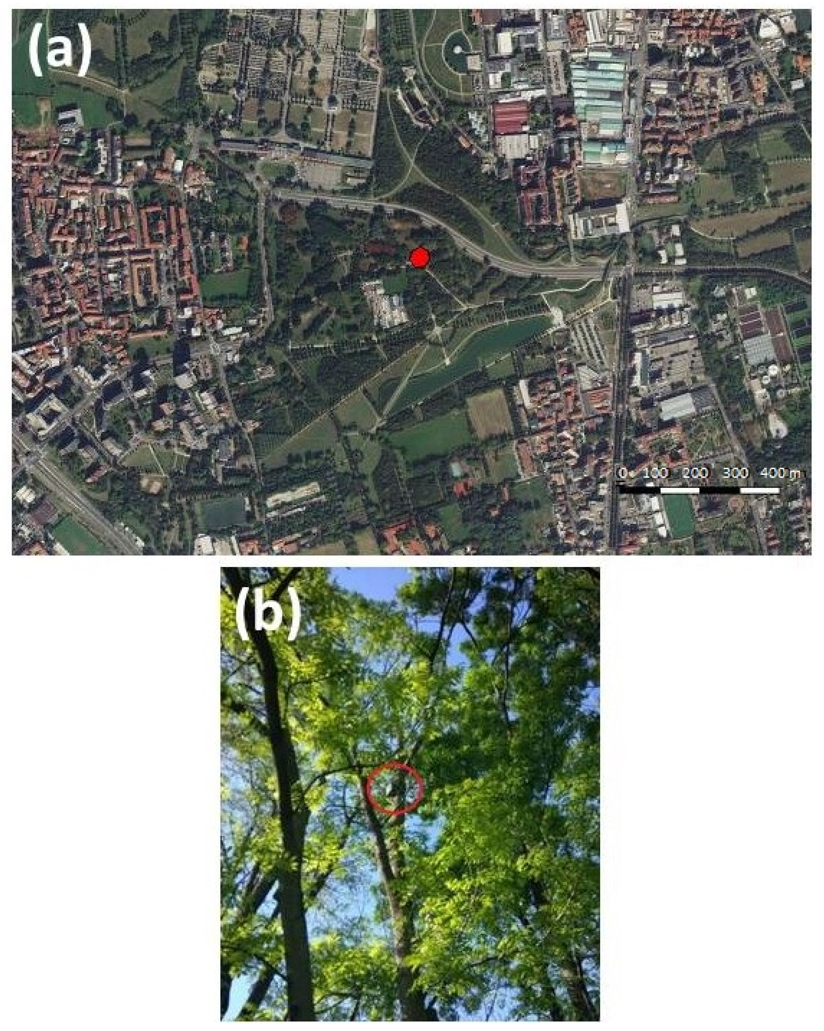
The recording period and frequency can be written and stored on an SD card according to a predefined schedule. Figure 1a shows the position of the SET recorder inside the park, located near the Bruzzano cemetery, in a suburban context. The land coverage of this area is quite green, with the widespread presence of roads (ranging from pedestrian paths within green areas to main arterial roads), activities and residential areas. The SET recorder was mounted on a tree at a height of five metres, as shown in Figure 1b.

The recorder position was approximately 90 m from a peri-urban arterial road with continuous road traffic noise emissions; more specifically, the daily mean traffic flow was approximately 22,000 vehicles (this number is the result of the following acoustic equivalence: a light commercial vehicle is equivalent to four cars and a heavy vehicle is equivalent to eight cars), the estimated mean traffic speed is approximately 50–60 km/h, with very rare congested flow events. The eastward direction of the road is the nearest to the measurement site, and it showed a peak of vehicles at 8 a.m.

2.2. Calculation of Eco-Acoustic Indices

The first step in data processing is to determine the main acoustic metrics to characterize the sound and start the calculation of the eco-acoustic indices. There are a wide variety of metrics used in the data analysis. One of the most commonly used is the Power Spectral Density (PSD). This estimates the strength of the variations in energy as a function of frequency. It is determined for each recorded audio file by applying the FFT algorithm (Fast Fourier Transform). The acoustic metrics obtained are used to calculate different eco-acoustic indices. Indeed, these indices are obtained through the post processing of sound frequencies and levels to bring out specific characteristics of environmental sound. In the analysis, we used the following seven indices:

• Acoustic Complexity Index (ACI)
• Acoustic Diversity Index (ADI)
• Acoustic Evenness Index (AEI)
• Bio-acoustic Index (BI)
• Acoustic Entropy (H)
• Normalized Difference Soundscape Index (NDSI)
• Dynamic Spectral Centroid (DSC).

The analysis and computation of eco-acoustic indices was performed in the “R” environment, version 3.5.1 [23]. In particular, Fast Fourier Transform (FFT) was computed by the function spectro available in the R package “seewave” [24], setting, as frequency bounds, the interval between 100 Hz and 24 kHz with computation based on 1024 points. This setting corresponds to a frequency bin of F = 46.875 Hz and, therefore, a time resolution $T_R=1/F=0.0213$ s. All the indices presented in this paper were computed using the R package “soundecology” [25], except the Dynamic Spectral Centroid (DSC) for which a script running in the “R” environment was specifically developed.

2.3. Loudness

To grasp how the noise recorded could be related to human perception, we evaluated the loudeness. Loudness is the subjective perception of sound pressure or the attribute of auditory sensation in terms of which sounds can be ordered on a scale extending from quiet to loud [26]. The relation of physical attributes of sound to perceived loudness consists of physical, physiological and psychological components.

The perception of loudness is related to the sound pressure level (SPL), frequency content and duration of a sound [27]. The relationship between the SPL and loudness of a single tone can be approximated by Stevens’s power law in which SPL has an exponent of 0.67. A more precise model, known as the Inflected Exponential function [28], indicates that loudness increases with a higher exponent at low and high levels and with a lower exponent at moderate levels [29]. The calculation of the loudness required the SET recorder to be calibrated. The calibration was performed by recording a white noise and a Class 1 B&K 2250 sound level meter and comparing the measured $Leq$ level.

2.4. Statistical Analysis

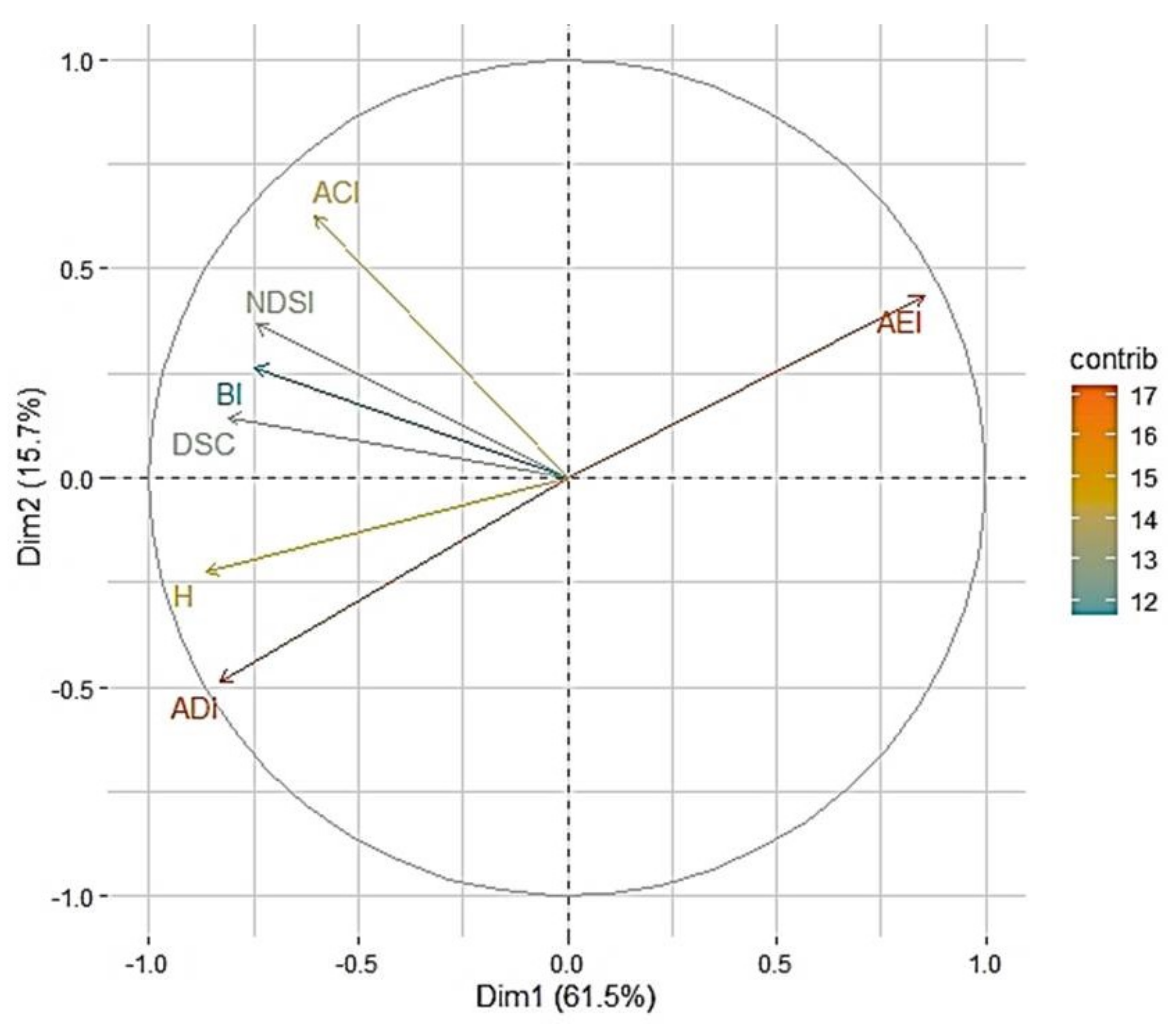
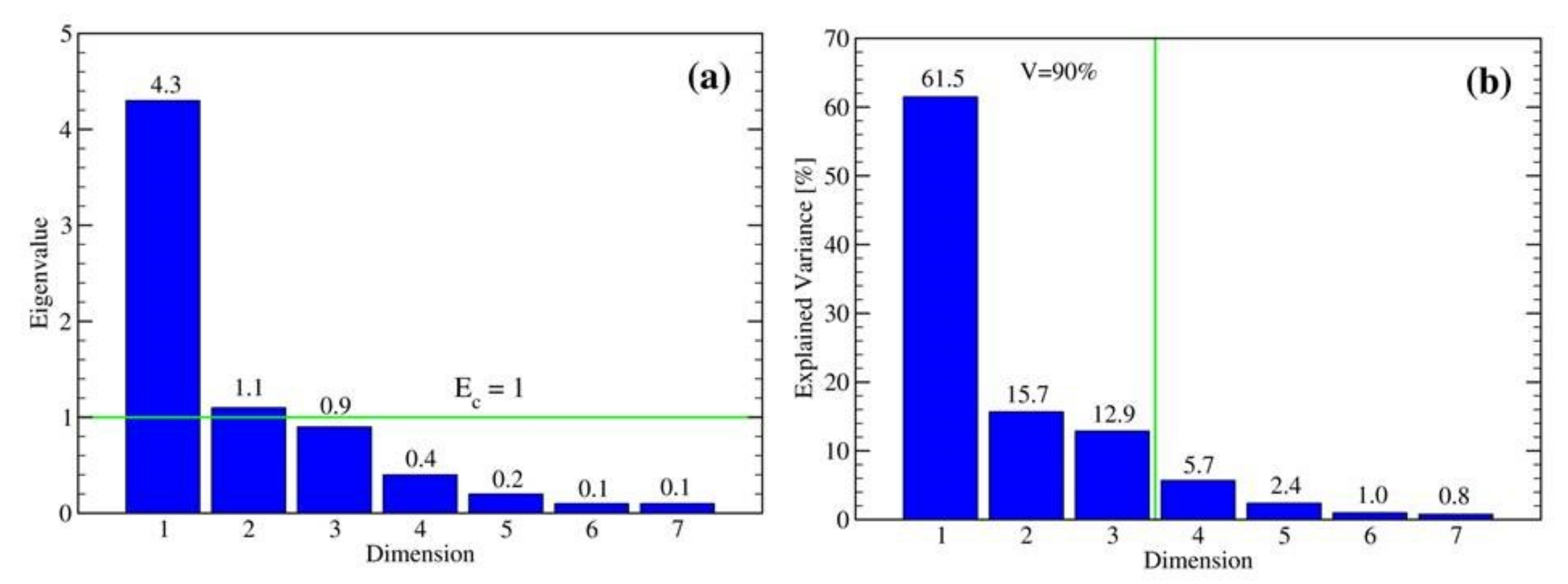
Before analysing the computed eco-acoustic indices, we performed a principal component analysis (PCA) on the input dissimilarity (distances) matrix of order 4312 (616 observations times seven variables) to reduce the number of variables and account for the largest possible variance of the original variables [30].

The method generates a new set of variables, called principal components, and each principal component is a linear combination of the original variables. All the principal components are orthogonal to each other, and thus there is no redundant information. Components with larger variance are the most relevant to the clustering, and therefore removing features with low variance acts as a filter that results in a distance metric that provides a more robust clustering.

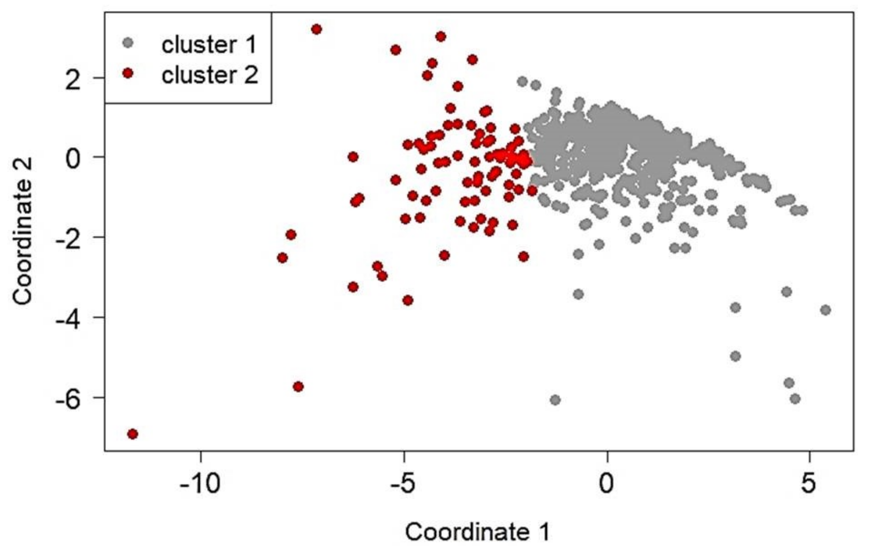
In order to find out patterns in our group of recordings, we decided to apply a cluster analysis on the entire set of data based on the most significant combination of variables. Given the large number of available algorithms, deciding which clustering method to use and the most appropriate number of clusters for the data can be a daunting task. Thus, we applied the package “clValid” [31,32,33] containing a variety of methods for the validation of the results from a cluster analysis. The available validation measures fall into the three general categories of ‘internal’, ‘stability’, and ‘biological’. For the scope of our study, the latter was not considered.

2.5. Aural Survey

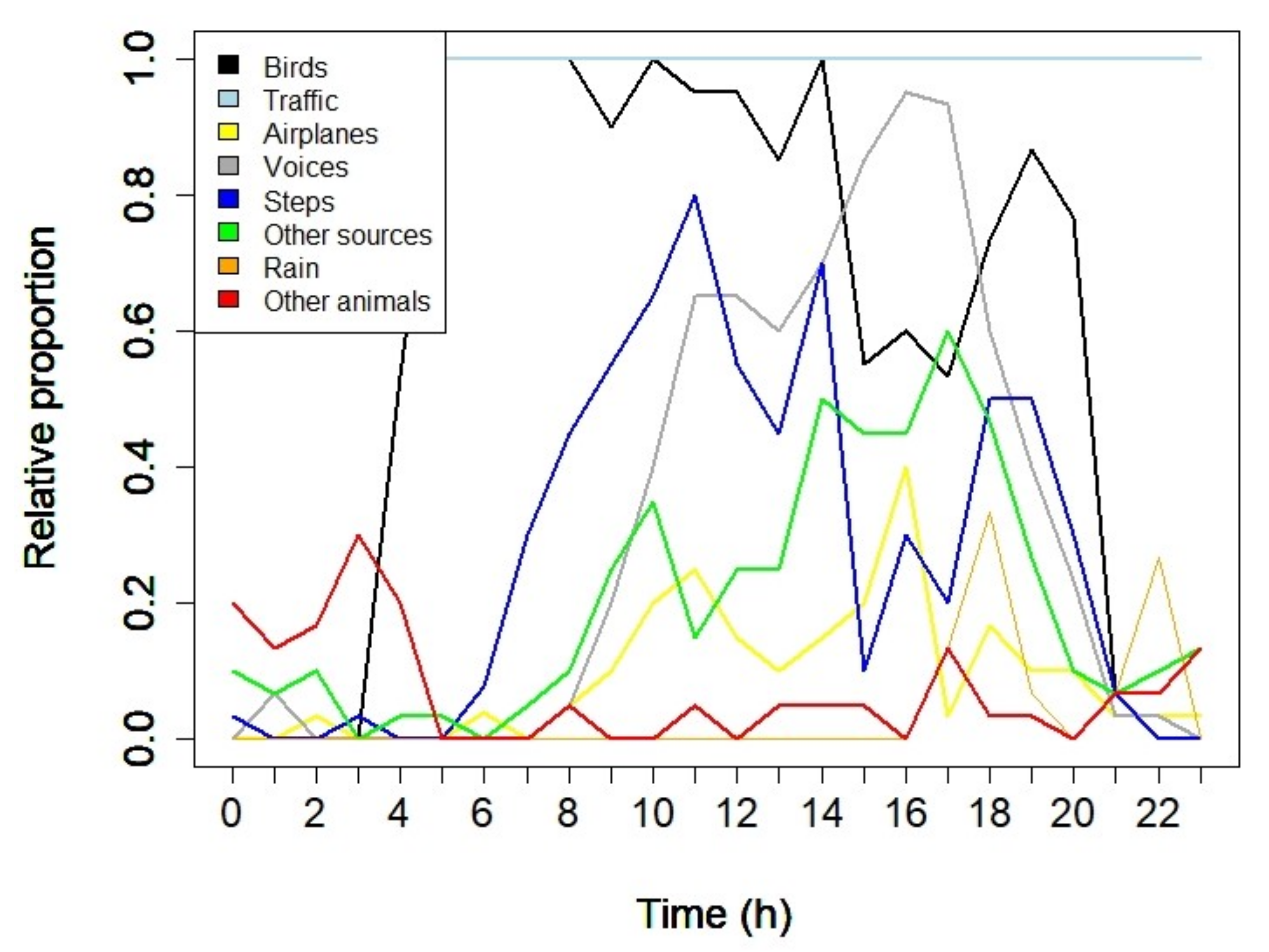
In this subsection, we report the scheme adopted for the aural analysis of all audio recordings. Each of 616 audio recordings was carefully listened to in order to capture distinguishing sound categories. Different sounds were previously identified in order to reach a consensus over the categories to be recognized and to select the most meaningful for our purposes.

In particular, we focused on determining biophonic activities (mainly avian vocalization and other animals), characteristics of technophonies sources (mainly road traffic noise and airplane fly-bys), human presence (voices and steps) and geophonies (rain and wind).

Table 1. Sound sources considered in the aural survey.

Categories	Sound Sources
Biophony	birds, dogs, frogs
Technophony	road traffic noise, sirens, mower, fireworks
Geophony	rain, wind
Antropophony	voices, steps

reports all the considered sources. One operator only was involved in listening to the recordings to avoid different perceptions due to individual hearing sensitivities.

In

Table 2. Indicators and corresponding sub-categories adopted for biophonic sources.

Perceived Indicators	Sub-Categories
Singing abundance	No birds		Few birds		Many birds
Singing distance	No birds		Close		Far
Singing activity	0%	(0–25]%	(25–50]%	(50–75]%	(75–100]%

and

Table 3. Indicators and corresponding sub-categories adopted for technophonic sources.

Indicators	Sub-Categories
Traffic distance	Close	Far
Traffic characteristics	Continuous	Intermittent

the indicators and the corresponding sub-categories are illustrated for both biophonic and technophonic sources (road traffic noise). Each sub-category is of straightforward interpretation. For only the perceived singing activity, the figures appearing in Table 2 refer to the percentage of singing activity occupation in each 1-minute recording. For the other sound sources, we indicated only the presence or absence in the audio recording.

3. Results

3.1. Results of the Cluster Analyses

As explained above, a PCA was performed in order to reduce the number of clustering variables and obtain an insight about the variable relevance. The results for the seven variables show that dimensions $d=1$ and $d=2$ have eigenvalues $E_i\ge 1$, (Figure 2a). The value $E_c=1$ is commonly used as a cut-off in order to decide which principal components to retain.

The cumulative percentage of variance, V, explained by these two principal components is $V_1+V_2=(61.5+15.7)\%=$ 77.2% (Figure 2b). In order to assure a cumulative percentage of variance greater than 80%, also the third principal component has been retained. In this case, the total explained variance is $V_1+V_2+V_3=$ 90.1%. Therefore, we use, hereinafter, the first three components (or eigenvectors, here denoted as dimensions) of the PCA.

Figure 3 shows the correlation plot representing the contributions of the variables in accounting for the variability of the first two principal components. It indicates that dimension 1, describing 61.5% of the data variability, is mostly associated with H (17.3%) and AEI (16.9%), whereas ACI, ADI, contributes to dimension 2 with 35.9 and 21.7%, respectively.

Table 4. Contributions of each eco-acoustic index to the first three principal components (dimensions).

Contribution (%)	ACI	ADI	AEI	NDSI	BI	H	DSC
Dimension 1	8.5	16.0	16.9	12.9	13.0	17.3	15.3
Dimension 2	35.9	21.7	17.2	12.2	6.4	4.6	1.9
Dimension 3	8.3	0.0	0.1	27.3	30.0	7.2	27.0

shows also the contribution of different variables to dimension 3 (not shown in Figure 3). In this case, BI and NDSI provide a contribution of 30% and 27.3%, respectively.

As shown in Figure 3, ADI and AEI are anti-correlated. This is a consequence of their formulation based on the Shannon [20] and Gini [21] indices, respectively. They were originally developed under the assumption that ADI and AEI would be, respectively, positively and negatively associated with habitats characterized by a more even distribution of sounds (increasing diversity). Contrary, ADI (AEI) and ACI are not correlated (their relative angle is close to 90${}^{\circ }$).

The first three PCA components were taken as input for the subsequent cluster analysis. Therefore, by applying the clValid cluster ranking algorithm, we found, as the optimal clustering algorithm, the hierarchical agglomeration with Ward’s method at two clusters [34]. Figure 4 illustrates the multi-dimensional scaling (MDS) results applied to the clustered data to provide a visual representation of the pattern of proximities among the data [35]. The distinction between clusters, marked by different colours, is rather satisfactory, though the two groups are not so clearly separated. Figure 5 illustrates the boxplots of the original eco-acoustic indices split into the two clusters.

As can be clearly seen, the statistical analysis based on a reduced number of dimensions was able to separate the indices quite efficiently. This result reflects the robustness of the clustering after dimension reduction. In particular, cluster 1 presented, in general, lower index values, the expression of less frequency modulation (ACI) and higher frequency diversity (ADI; opposite trend for AEI). ADI measures the entropy in frequency space. Keeping in mind that higher ADI values indicate greater flatness across frequency bands and lower ADI values indicate a sharper distribution of frequencies, this result could be associated with the presence of a higher variety of frequencies in the cluster 2 dataset.

The NDSI index ranged between −1 and +1 with values close to −1 unbalanced towards low frequencies and values close to +1 with a prevalence of high frequencies. NDSI together with DSC provide useful information on the frequency content of recordings and allows a straightforward interpretation. Indeed, cluster 1 presents lower frequency components (NDSI and DSC median values −0.96 and 0.42 kHz, respectively; see

Table 5. Median values of the eco-acoustic indices in cluster 1 and 2. Note that the first six indices are adimensional, while DSC is in kHz.

	ACI	ADI	AEI	NDSI	BI	H	DSC (kHz)
Cluster 1	151.34	5.74	0.79	−0.96	68.49	0.60	0.42
Cluster 2	163.15	6.17	0.68	−0.81	90.75	0.66	0.76

), whereas cluster 2 shows higher median values (−0.81 and 0.76 kHz).

The two clusters appear well separated, but the calculated values are low in any case. This result indicates a strong presence of low frequency sources. BI represents the area under the mean frequency spectrum; thus, it provides a measure of both the frequency content and the sound level. In this case, the result shown in Figure 5 reveals a lower frequency abundance and levels for cluster 1 compared to cluster 2.

The acoustic entropy index, H, measures entropy in both time and frequency space. H ranges from H = 0 for pure tones, to H = 1 for high-energy, evenly distributed sound. Higher values are generally associated with higher species richness. In our case, cluster 2 presents H median values of 0.66, i.e., 10% higher than cluster 1, as a result of higher variability in space (ADI) as well as in time domain.

3.2. Results of the Aural Survey

In this subsection, we present the results of the aural survey in terms of distribution of the categories listed in Table 1, Table 2 and Table 3. Figure 6 reports the relative proportion of perceived bird‘s activity throughout the day as classified by a trained operator. The result shows an abundance of bird activity (morning chorus) between 5:00 a.m. and 8:00 a.m., the presence of few singing birds throughout the day with a peak between 14:00 and 15:00, and a complete absence of bird activity during the night time.

Regarding the road traffic distance and characteristics, the traffic noise is perceived as far and intermittent just during the night period; whereas, during the daytime, it is perceived as close and continuous (see Figure 7 and Figure 8). Comparing this evidence emerging from aural surveys with computed traffic volumes of the nearest arterial road, we can observe that the trends are correlated.

Indeed, as reported in Figure 9, the hourly flow was very low during the night period, in particular it was near null from midnight until 5 a.m. In this time interval, the traffic noise contribution came from distant roads or from sporadic vehicular passages from the near arterial road. In the remaining period of the day, the traffic flow in the closest road, even though highly fluctuating, maintained sufficiently high levels to generate the perception of a continuous noise.

Figure 10 describes the relative proportion of each perceived source throughout the day. The proportion refers to the 1-h cumulative presence of the sub-category in each 1-min recording. The other option is the absence of the source. Traffic was always present (either close or far, see also

Table 6. The total occurrences and corresponding percentage (by dividing the total occurrence by 616) found in the aural survey.

	Birds	Traffic	Fly-by	Voices	Steps	Other Sources	Rain	Other Animals
Total	338	616	48	170	148	118	26	49
%	55	100	8	28	24	19	4	8

) as well as bird activity—however, this was limited to the daytime hours. Rain was the only geophony detected (no wind) and was partially present only during the late afternoon and evening hours.

Human presence was observed from 7:00 to 19:00 hours as well as the presence of other sources due to human activity (sirens, mower and fireworks). The major contribution during the nighttime was due to other animal vocalizations (mainly frogs) and birds in the early morning. Peaks of human presence (voices) corresponded to a decrease of bird activity during the afternoon hours. As a summary, Table 6 reports the occurrences of the considered events in the aural survey. Avian activity is the second by frequency with 55% of observations followed by human activity split into voices, steps and other sources.

3.3. Results of the Loudness Evaluation

In order to provide indications on how the noise recorded at the site of study may be perceived by humans, we concentrated on those recordings showing the highest values of eco-acoustic indices.

Table 7. Time of the recording, highest eco-acoustic index, mean loudness, $〈N〉$ and the difference between the 5th and 50th percentile of loudness, $N5-N50$.

Date and Time of Recording	Maximum Value of Eco-Acoustic Index	$〈\mathit{N}〉$ (Sone)	$\mathit{N}5-\mathit{N}50$ (Sone)	Sound Sources
30 April 2019 17:42	ACI (217.48)	10.5	11.3	Close and continuous traffic, voices, other sources
2 May 2019 22:12	ADI (6.71); AEI (0.39); H (0.76)	8.3	2.3	Close and continuous traffic, rain
1 May 2019 10:36	NDSI (0.25); DSC (2.46 kHz)	6.2	4.8	Close and continuous traffic, few/close birds, (bird activity >50–75), steps
1 May 2019 12:12	BI (131.35)	10.7	7.3	Close and continuous traffic, many/close birds, (bird activity >75), steps

, reports the time of recording, the indication of the highest eco-acoustic index, the mean loudness, $〈N〉$ and the difference between the 5th and 50th percentile of the loudness, $N5-N50$.

Table 7 shows how both the presence of voices (first recording) and bird activity (last recording) were able to provide both high values of loudness and high fluctuation of loudness (see $N5-N50$ difference). As an example, Figure 11 illustrates the loudness spectrogram for a 1-min long recording, on 1 May 2019 at 12:12. Here, the presence of many and close birds (bird activity >75) increases the loudness indicator.

4. Discussion

The results shown in Section 3 reveal the good performance of the statistical analysis to discriminate among different recordings based on selected combinations of eco-acoustic indices. The obtained clusters are characterized by different distributions of such indices. These differences require further attention.

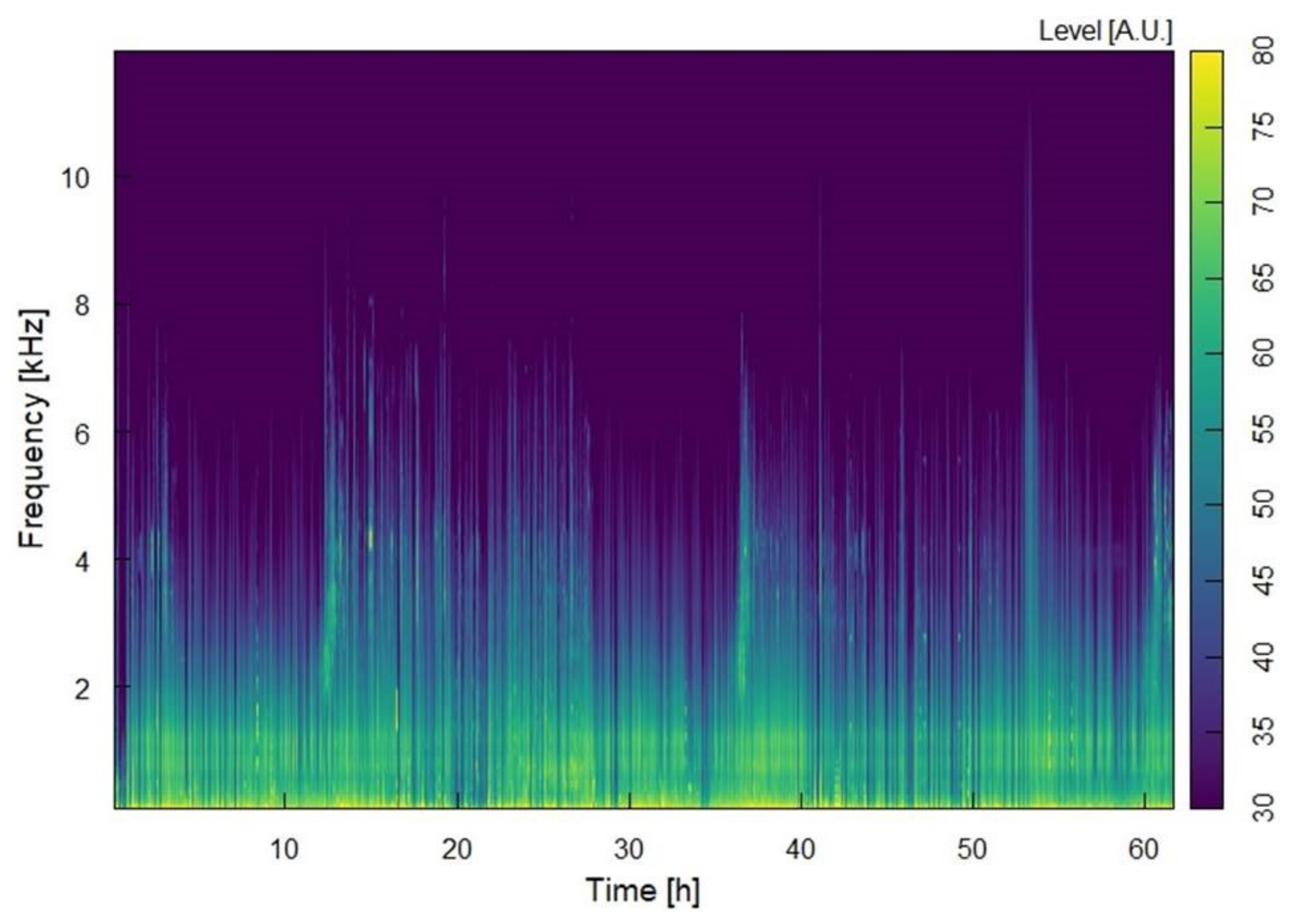
First, we computed the mean spectrogram for each recording. In this case, we used a frequency range (0.1–12) kHz and 1024 points as the window length for the analysis. The results are shown in Figure 12. Here, we can observe an intense frequency band at low frequencies up to approximately 1.5 kHz, which is most likely associated with traffic noise and less intense at higher frequencies, up to (8–10) kHz. The latter is associated with sounds produced by biophonic activity.

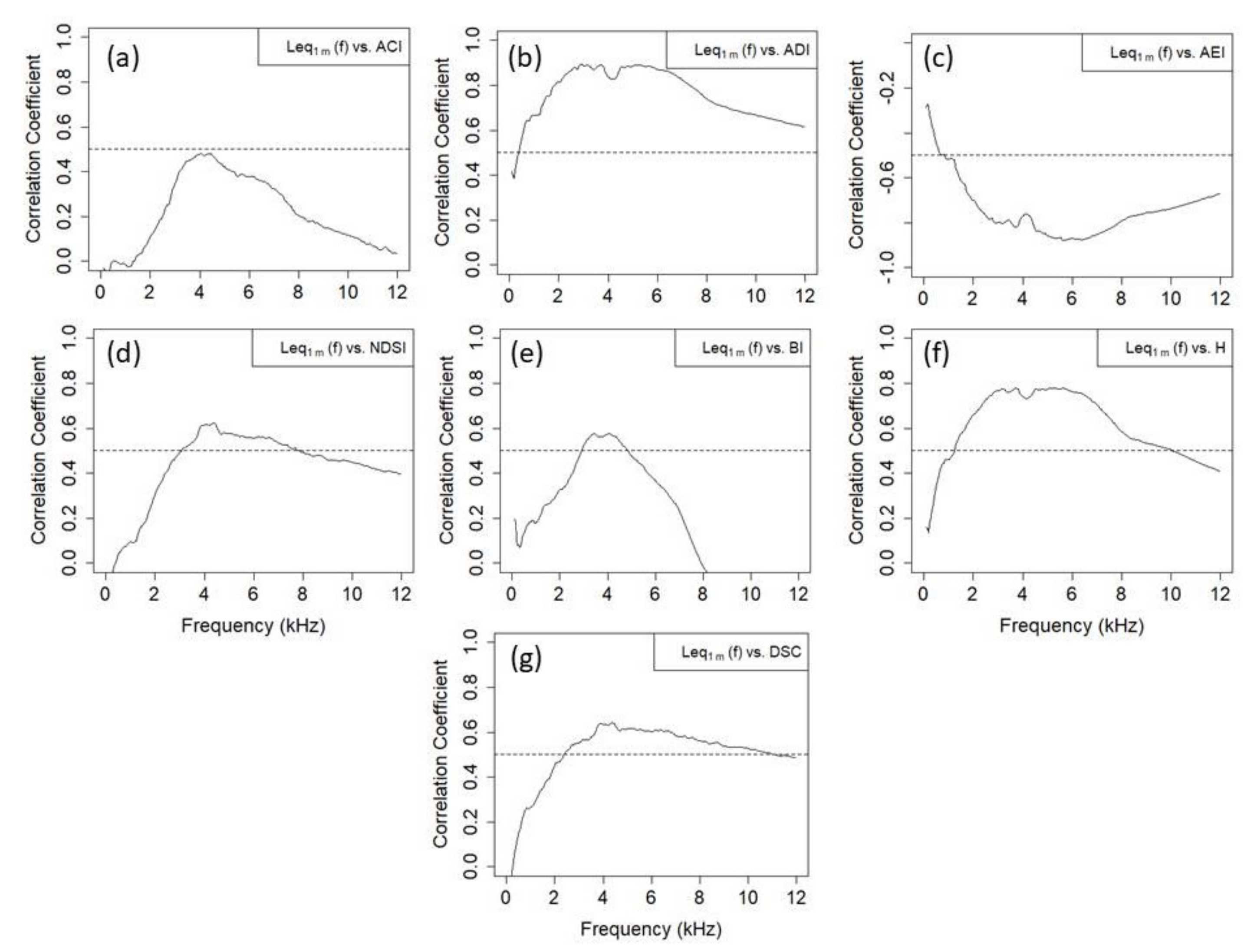
In order to understand what frequencies better describe such complex spectrogram pattern in terms of defining an environmental quality indicator, we performed a Pearson’s correlation coefficient computation between the level time series at a given frequency k and each index time series.

$$C_k=\frac{1}{N_t}\sum _{n=1}^{N_t}\left(\frac{Leq\left(f_{k,n}\right)-〈Leq\left(f_k\right)〉}{{\sigma }_{\mathrm{f}}^2}\right)\left(\frac{Inde{x}_n-〈Index〉}{{\sigma }_{\mathrm{Ind}}^2}\right),$$

(1)

where $N_t$ is the time series length, k is the kth frequency, with $k\in$ [0.1–12] kHz and ${\sigma }^2$ as the corresponding variances. The results are displayed in Figure 13.

We can clearly see how each index presents a maximum of correlation for frequencies above 2 kHz. In particular, ACI and BI present a peak distribution with a maximum at approximately 4 kHz, rapidly falling upwards. The other indices present a correlation coefficient that remains quite high even at frequencies of 10–12 kHz. The correlation coefficient for ACI is below 0.5 (see dashed line in Figure 13); whereas, for AEI, the results are anti-correlated with the frequency (minimum at frequencies greater than 2 kHz). This result suggests that the considered indices were able to capture most of the sound characteristics associated with biophonic activities (no-traffic component).

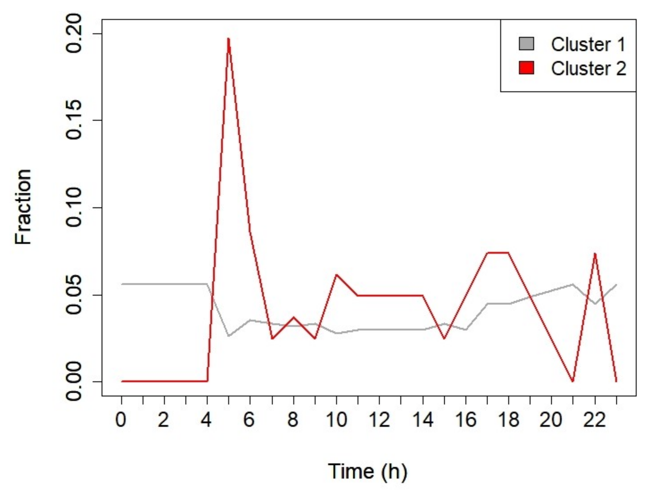
In order to validate the cluster analysis in terms of the discerning capability between different bird activities, we first looked at the cluster composition in terms of the different recording time. The results are shown in Figure 14. Here, we can clearly see how cluster 2 presents a peak of recordings during the morning chorus and the afternoon. No recordings were observed during the night period. On the contrary, cluster 1 includes recordings that were evenly distributed throughout the hours of the day and the night period (slightly higher in the latter).

We also checked for all the aural survey characteristics highlighted by the trained operator. In particular, Figure 15 reports the singing activity quantified as the percentage of singing presence in the audio recording time. About 50% of cluster 1 is made of recordings with a complete absence of bird activity with a minimum of about 10% in the interval >(50–75)% and >75% of singing activity. Cluster 2 presents a maximum of approximately 40% of recordings with singing activity above 75%.

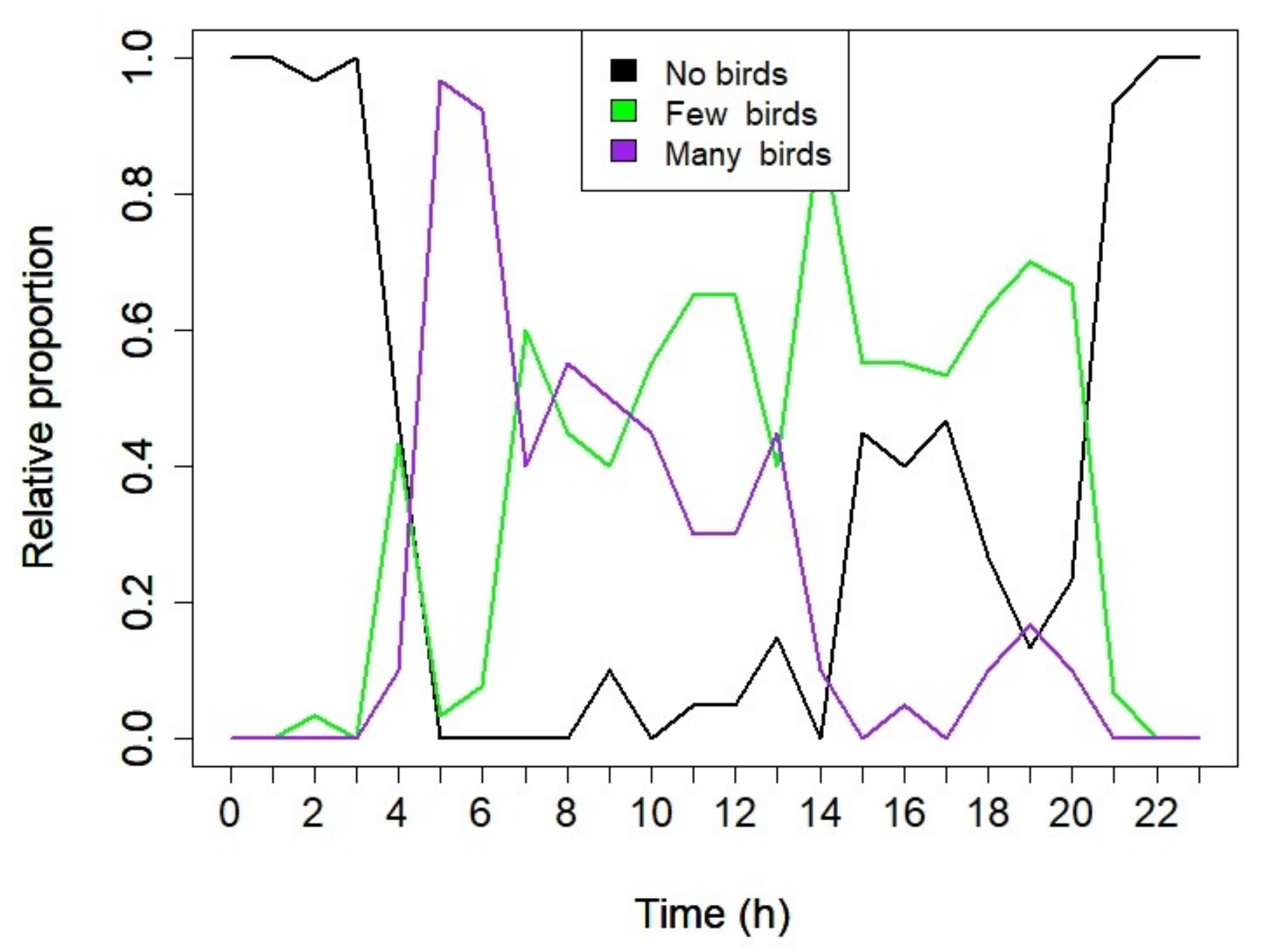
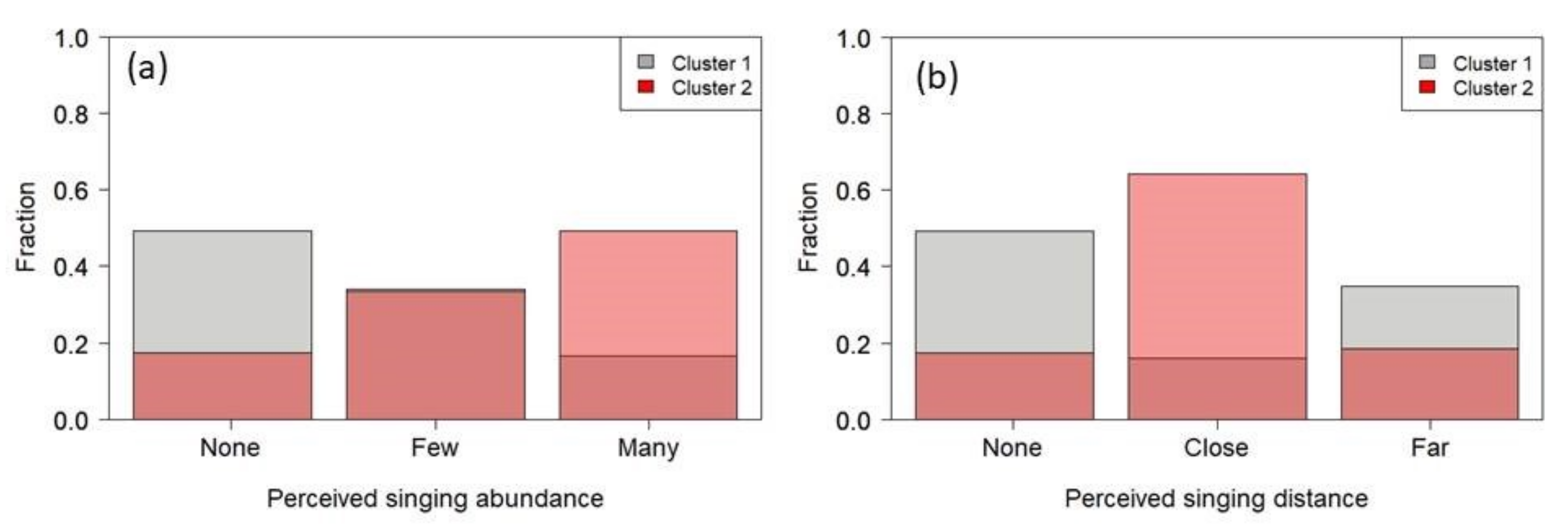
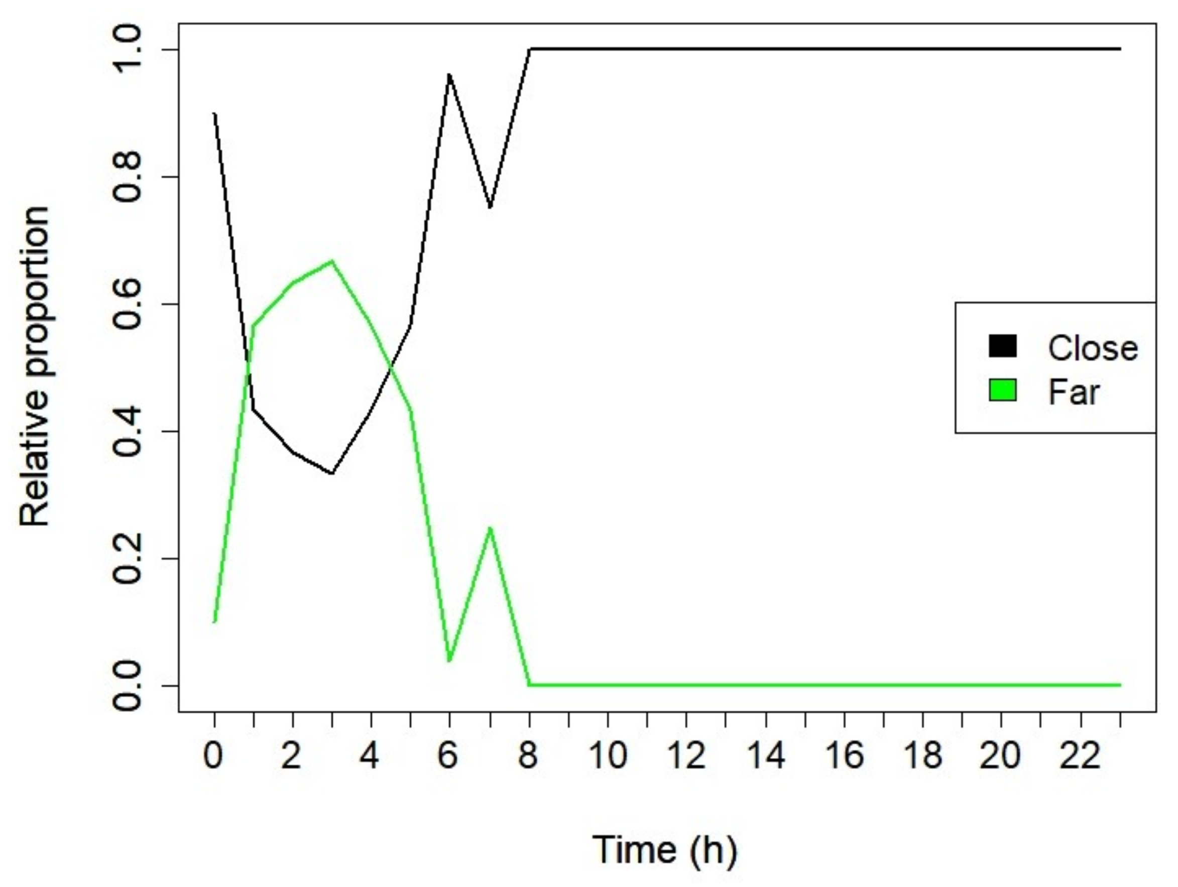
The perceived singing abundance in the two clusters, shown in Figure 16a, confirmed the previous results: an absence of activity for the majority of recordings in cluster 1 (∼50%), many bird singings in the majority of cluster 2 (∼50%) and few bird singings equally distributed in the two clusters. Regarding the perceived singing distance, cluster 1’s composition was made of audio recordings with either an absence or far singing activity; whereas, in cluster 2, we found recordings where the singing activity was perceived as close (see Figure 16b).

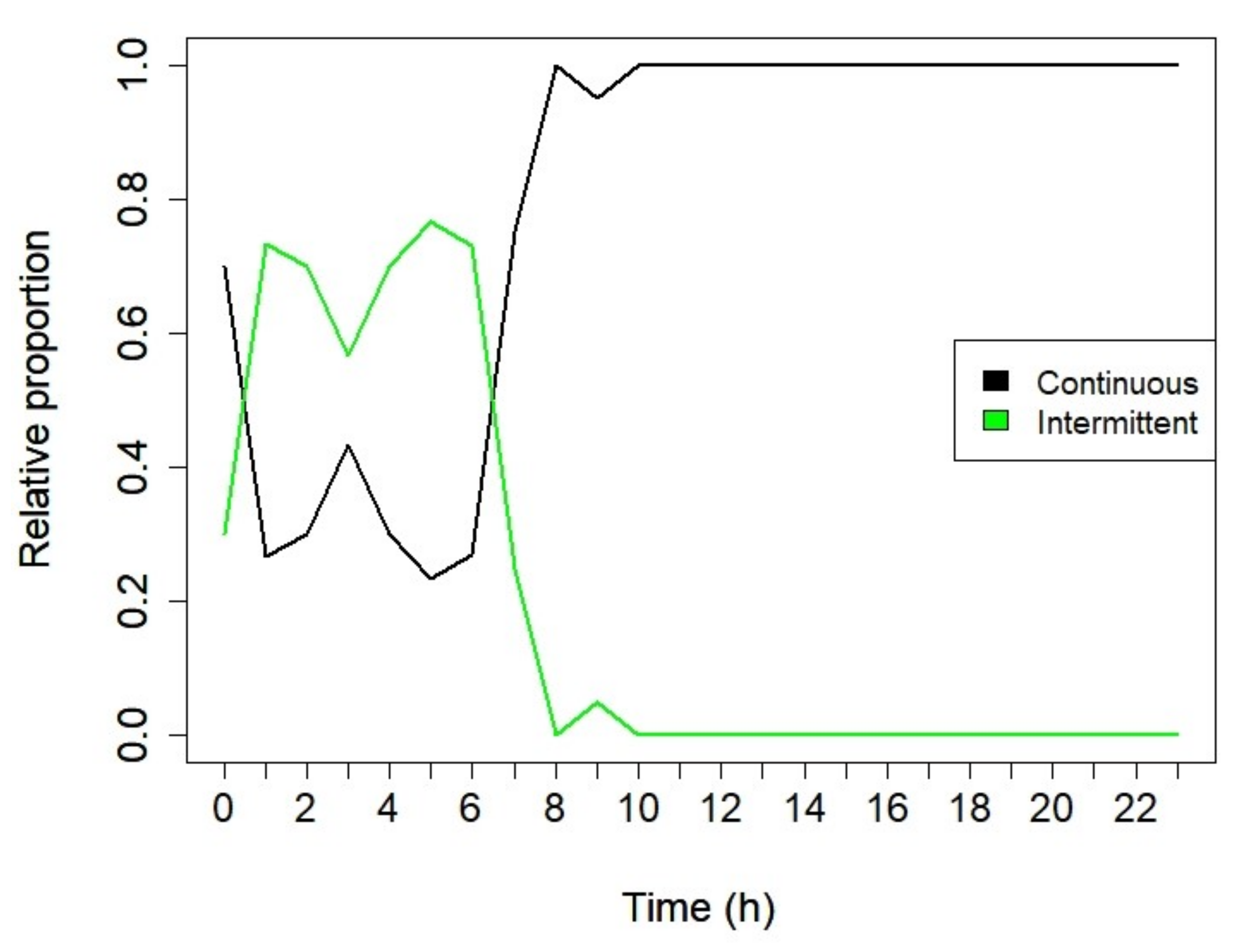
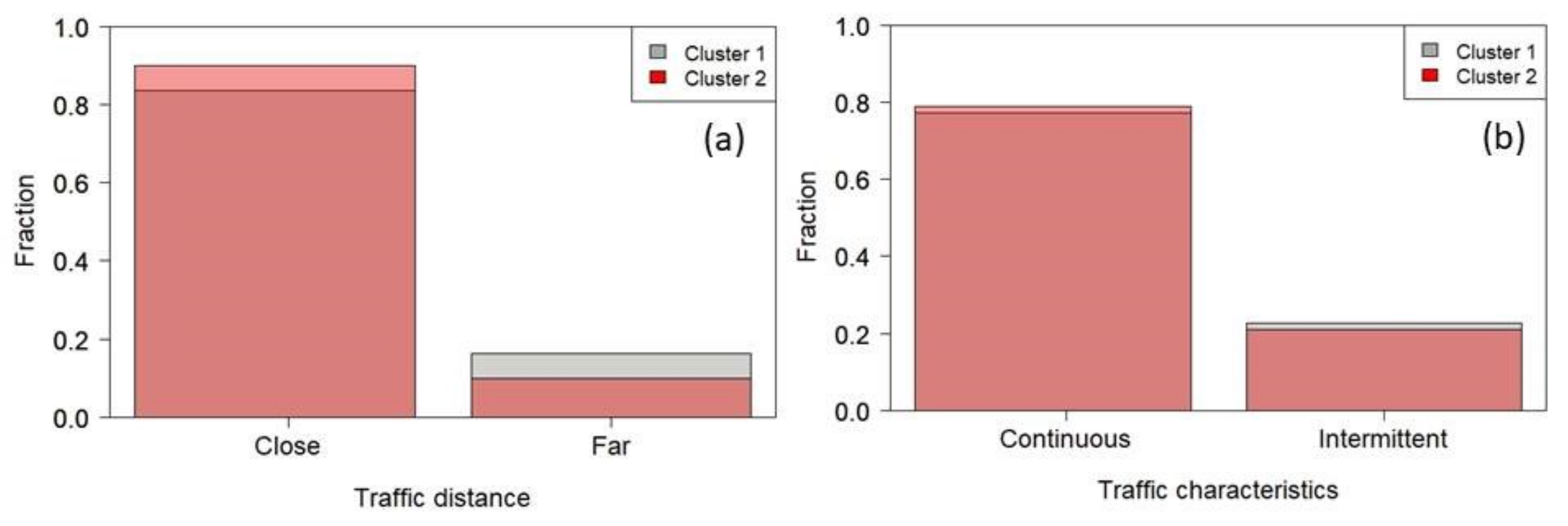
Figure 17a,b reports the distribution of audio recordings in the two clusters versus the presence of traffic perceived in terms of two categories: distance and dynamic characteristics. The results indicate that both clusters presented the majority of audio recordings characterized by close perceived distance and continuous traffic noise characteristics. As a summary,

Table 8. Percent [%] allocation of occurrences in each cluster.

Allocation (%)	Birds	Traffic	Fly-by	Voices	Steps	Other Sources	Rain	Other Animals
Cluster 1	51	100	8	24	22	17	4	8
Cluster 2	82	100	6	48	36	32	9	5

reports the allocation of occurrences in each cluster. As for the presence of bird vocalization, both many and few bird activity levels were accounted for. The presence of voices as well as the sub-category of other sources were unbalanced towards cluster 2, meaning that they may have some contribution to the cluster formation.

These results suggest that the adopted analysis was able to discern among a complexity of sound sources based on the selection of a combination of eco-acoustic indices. These indices can efficiently separate audio recordings characterized by different degrees of biophonic activity in terms of the temporal distribution, biophonic intensity and richness as identified by an aural survey. This discrimination capacity was not influenced by the presence of continuous and close traffic noise sources, which were found in both groups of audio-recordings.

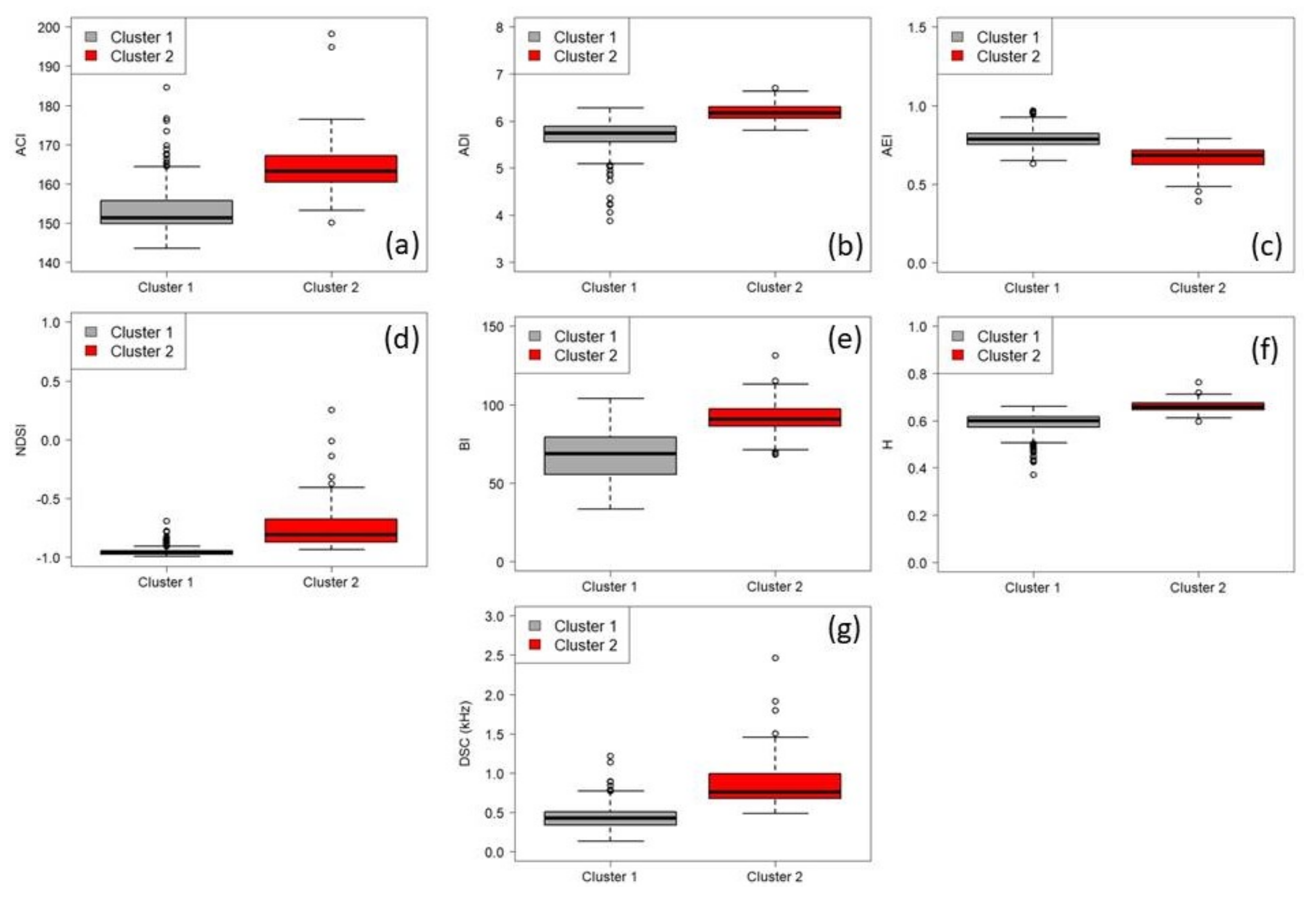
These characteristics are well reflected in the boxplots illustrated in Figure 5 for the two clusters obtained from the combination of all the considered eco-acoustic indices. The presence of biophonic activity was effectively captured by the ACI index sensitive to frequency and time modulation typical of birds’ singing. The presence in cluster 2 of both biophonic and anthropogenic activities, hence, with a wider frequency composition, implies higher values of the ADI index (opposite consideration for AEI). This result was confirmed also by the acoustic entropy index, H, which measures entropy in both time and frequency space.

In this case, cluster 2 presented higher H values as a result of higher frequency occupation in space domain (as ADI does), as well as a more uniform distribution of amplitudes in time domain. For the same reason, the BI values were higher in cluster 2 because of the overlapping of the two major sound sources: traffic noise and singing activity, as this index is sensitive to both the amplitude and number of occupied frequency bands. Complementary information is provided by NDSI and DSC indices. In this case, a more straightforward interpretation is possible.

Indeed, both clusters of audio recordings were characterized by NDSI values below 0. This result tells us that, even cluster 2, despite the presence of most of biophonic activity (generally, in the frequency range 2–8 kHz), was characterized by the presence of traffic noise sources (low frequency 0.1–1.5 kHz). The same pattern was found analysing the DSC index. The DSC was heavily affected by anthropogenic sources. As a comparison, NDSI and DSC indices calculated for audio recordings in pristine habitats like a bush area in the Appennino mountains (Italy), showed values approaching 1 for NDSI and 3 kHz for DSC [14,22].

This result alone is significant to establish a quality criterion for the examined urban park. The presence of highly congested roads (approximately 22,000 vehicles per day) at the borders of the urban park is reflected on the low quality ‘score’ obtained for NDSI and DSC especially when considering the group of audio recordings where biophonic activities are concentrated (cluster 2). As already mentioned, ACI, ADI (AEI), BI and H capture different aspects of the spectral characteristics and are fundamental to separate different dynamics linked to the time, intensity and species abundance. However, the quality of an environment is mainly driven by the frequency content that is typical of each habitat.

The statistical approach selects those combinations of indices carrying a greater content of information for the environment in terms of the dynamicity, frequency richness, frequency contribution and levels as captured by each single soundscape index. The subsequent cluster analysis highlights the periods of the day corresponding to higher eco-acoustic dissimilarity. Matching the cluster analysis results with the aural survey can help the identification of sound sources responsible for the soundscape degradation.

This method of analysis can, thus, be of great advantage in evaluating the environmental quality of urban parks especially when oriented to create noise-protected areas for both animals and humans. These areas may contribute appreciate and increase the awareness regarding the importance of urban–natural tranquil areas.

5. Conclusions

Urban parks are generally regarded as restoring areas in large cities. Medium–large size urban parks are often exposed to road traffic noise produced by the surrounding roads and to anthropogenic sounds due to the presence of people. Such non-natural sounds can easily alter the perceived soundscape quality of the park and, therefore, reduce its potential restorative function. Parco Nord in Milan, Italy is located in a strategic position, and it covers the function of “stepping stone”, that is, an area of passage and rest of birds towards and from the areas with the highest biodiversity.

Thus, the presence of background noise might interfere with the presence of biophonic activity due to either partial overlapping of frequencies or high background noise levels. In order to develop an analysis method for the eco-acoustic assessment of an urban park, we took an audio recording of approximately 60 h at a location characterized by the presence of surrounding roads. After the calculation of “traditional” eco-acoustic indices, we performed a cluster analysis on a selection of the original eco-acoustic indices based on PCA, in order to determine groups of recordings with similar sound environment.

The analysis proved to be robust, and the comparison of the obtained results provided a good matching with the aural survey by a trained operator. The overall quality of the examined site proved to be quite poor. Notwithstanding the presence of avian species, highlighted by the characteristic dawn chorus found in the assemblage of cluster 2’s audio recordings and characterized by higher eco-acoustic indicators, both clusters and especially cluster 2 revealed NDSI and DSC values that were heavily influenced by traffic sources.

This result, confirmed by the aural survey, suggests that the relative high values of ACI, ADI, BI and H though highlighting the presence of significant spectral dynamics and frequency abundance, the normalized index NDSI and the spectral centroid DSC can provide a more straightforward indication on the presence of traffic noise background. The good correlation between the unsupervised statistical analysis and the aural survey suggests the use of the former analysis to derive information on the environmental quality assessment over large areas by creating maps of eco-acoustic indices.

However, further measurements and studies are required to determine both time and spatial scales for the monitoring of eco-acoustic indices. Such information will be used to improve the use of the park, not only for orienteering the users toward areas with features more appropriate to their enjoyment and expectations but also to help the park authorities to plan mitigation measures and creat areas more hospitable for avian communities.