Exploring Wind Energy Potential as a Driver of Sustainable Development in the Southern Coasts of Iran: The Importance of Wind Speed Statistical Distribution Model

Abstract

Wind energy as a clean and inexhaustible source of renewable energy can be a key element of sustainable development that decreases dependence of countries on fossil fuels. Therefore, implementing accurate and comprehensive feasibility studies in countries with a high level of consumption of traditional energy resources is vital; an approach encouraged and supported by green funds and climate change action. It is also crucial to helping spur economic and sustainable growth of these countries. In this regard, this study aims at accurate evaluation of onshore wind energy potential in seven coastal cities in the south of Iran. Six Probability Distribution Functions (PDFs) were examined over representative stations. It was deduced that the Weibull function, which is the most used PDF in similar studies, was only applicable to one station. Here, Gamma distribution offered the best fit for three stations and for the other ones, Generalized Extreme Value (GEV) performed better. Considering the ranking of six examined PDFs and the simplicity of Gamma, it was identified as the effective function in the southern coasts of Iran bearing in mind the geographic distribution of stations. Moreover, six wind energy converter power curve functions contributed to investigating the capacity factor. It is found that, using only one function could cause under- or over-estimation. Then, stations were classified based on the National Renewable Energy Laboratory system. Last but not least, examining a range of wind energy converters enabled scholars to extend this study into practice and prioritize the development of stations considering budget limits.

1. Introduction

Renewable energies are harnessed in various types such as wind power, solar power, biopower, geothermal power, and ocean power. All these types, except geothermal and ocean energy, originate from the infinite energy of the sun, which emits the power about $1.74\times {10}^{17}\mathrm{w}$ [1]. Considering 1–2 percent of this energy is transformed into wind energy, it is an interminable, environmentally friendly, clean, and reliable source, which is 50–100 times higher than energy conversion from all the plants in the earth combined [2]. It is estimated that the global wind energy potential is about 10 million MW, which could fulfill 35% of the total demand for world energy [3]. The cumulative global installed capacity of wind energy was 539,581 MW in 2017, and it is forecasted that the global wind capacity will reach 800,000 MW by 2021 [4]. In another study, it was estimated that the wind share of electricity generation will rise from 3.5% in 2015 to 36% in 2050 [5] The initial goal of this study is to provide a comprehensive technical assessment of wind energy resources. This helps engineers, scholars, and policymakers to decide on optimal investment with maximum profits. Scholars and practitioners in the future could use the results of the current study as inputs for further economic analyses. Wind resource assessment is being conducted in seven coastal stations; including Abadan, Mahshahr, Bordekhoon, Delvar, Kish, Jask, Chabahar and the results are compared against similar studies.

This study is structured as follows. In Section 1.1 an overview of wind energy in Iran is provided. Section 1.2 presents a literature review of wind energy potential assessment in Iran. Section 2 depicts the area of study and characteristics of the sites. Section 3, explains the methodology used in the study, statistical distributions, determining wind power and energy density and capacity and availability factors of different wind turbines. Section 4 describes case studies and results of the study using different statistical distributions across all stations and wind power and energy density.

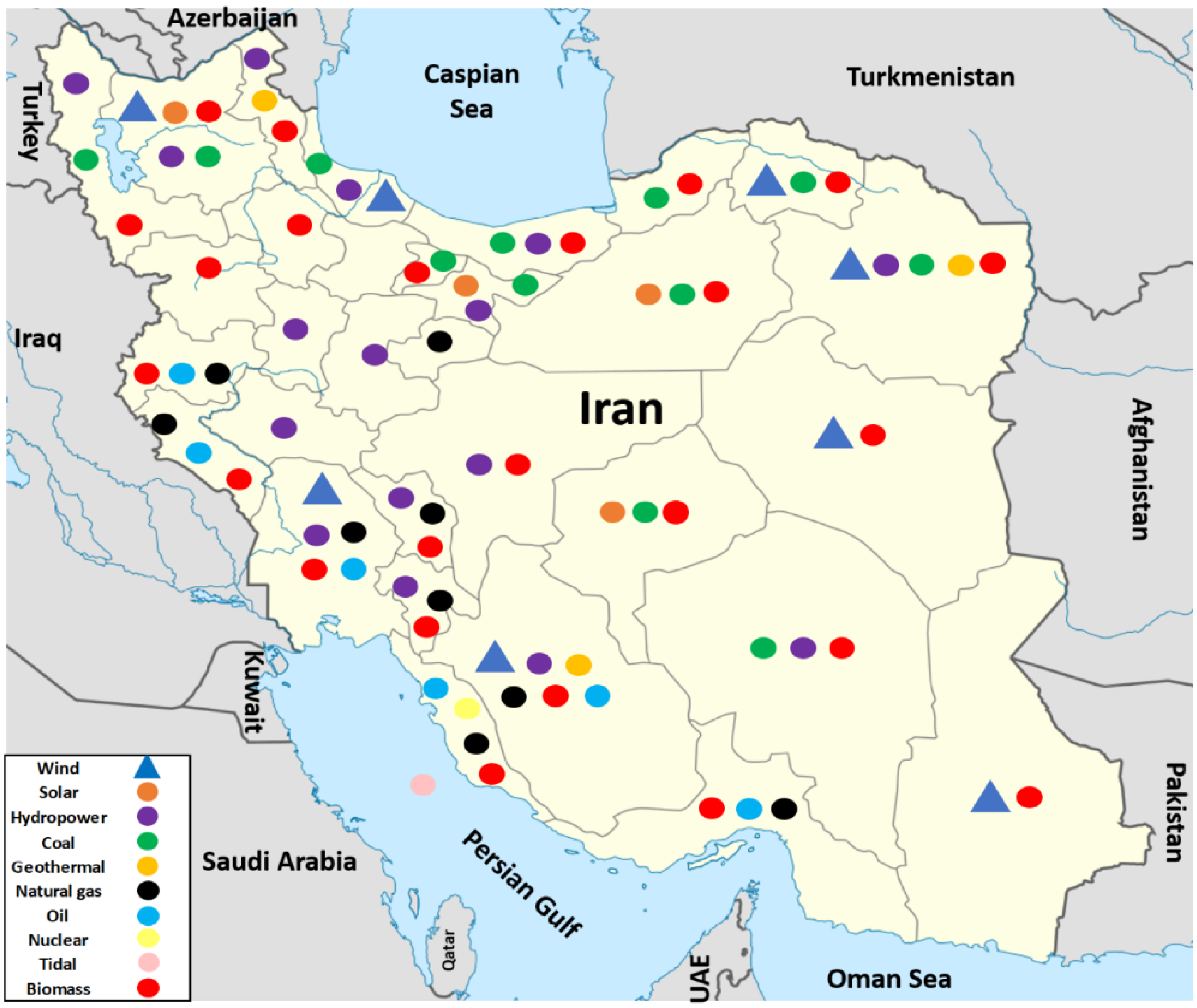
1.1. Wind Energy in Iran

Although Middle East countries are rich in conventional energy sources such as oil and natural gas, industrialization and environmental impacts have encouraged their policy-makers to invest in renewable energies [6]. Iran has a population of 79.2 million and an area of 1,648,195 km² (about half of this area is habitable), and largely depends on fossil fuels such as crude oil in its energy sector [7]. Now, there is a considerable consumption of traditional energy resources in Iran because of the large amount of low-cost fossil fuels [8]. This exacerbated the misuse of energy in industrial, transportation, and home sectors resulting in various environmental problems [9]. The situation compelled energy policymakers to move toward renewable energies in the country. The average growth rate of energy consumption and generation in Iran is 4% and 2%, respectively and therefore, it is expected that Iran increasingly will need to provide a great share of its energy demand from renewable energy sources in years ahead, to meet future rising energy demand [10]. As set out in the 6th national development plan of the country, the Iranian government has the target of extracting 5000 MW from renewable energy resources by 2020 [11]. Due to this high demand, extensive studies on different types of renewable energy should be considered [12].

However, Iran has great potential for solar energy production because of its dry and warm climate. Without industrial infrastructures to produce solar panels and difficulty in import materials and resources because of political conditions, starting large-scale solar power would be expensive and time-consuming. With these challenges, governments have drawn their attention to a more practical and accessible solution: Wind power. In 1994, the first wind turbine was installed in Iran at Manjil. After that, various efforts were made to increase the wind electricity generation in Manjil such as the construction of 25 MW and 60 MW power stations. In 2018, the total installed capacity of Iran’s wind energy reached 280 MW. According to the Ministry of Energy reports, Iran planned to reach a 4500 MW goal in wind energy capacity in 2023 [13]. Although wind energy shares 43% of Iran’s electricity production based on renewable energies (greatest among all other types) [14], as shown in Figure 1, there is a lack of installed wind capacity in Iran’s energy resources especially in southern coastal regions regarding their area and population.

1.2. Review of the Literature

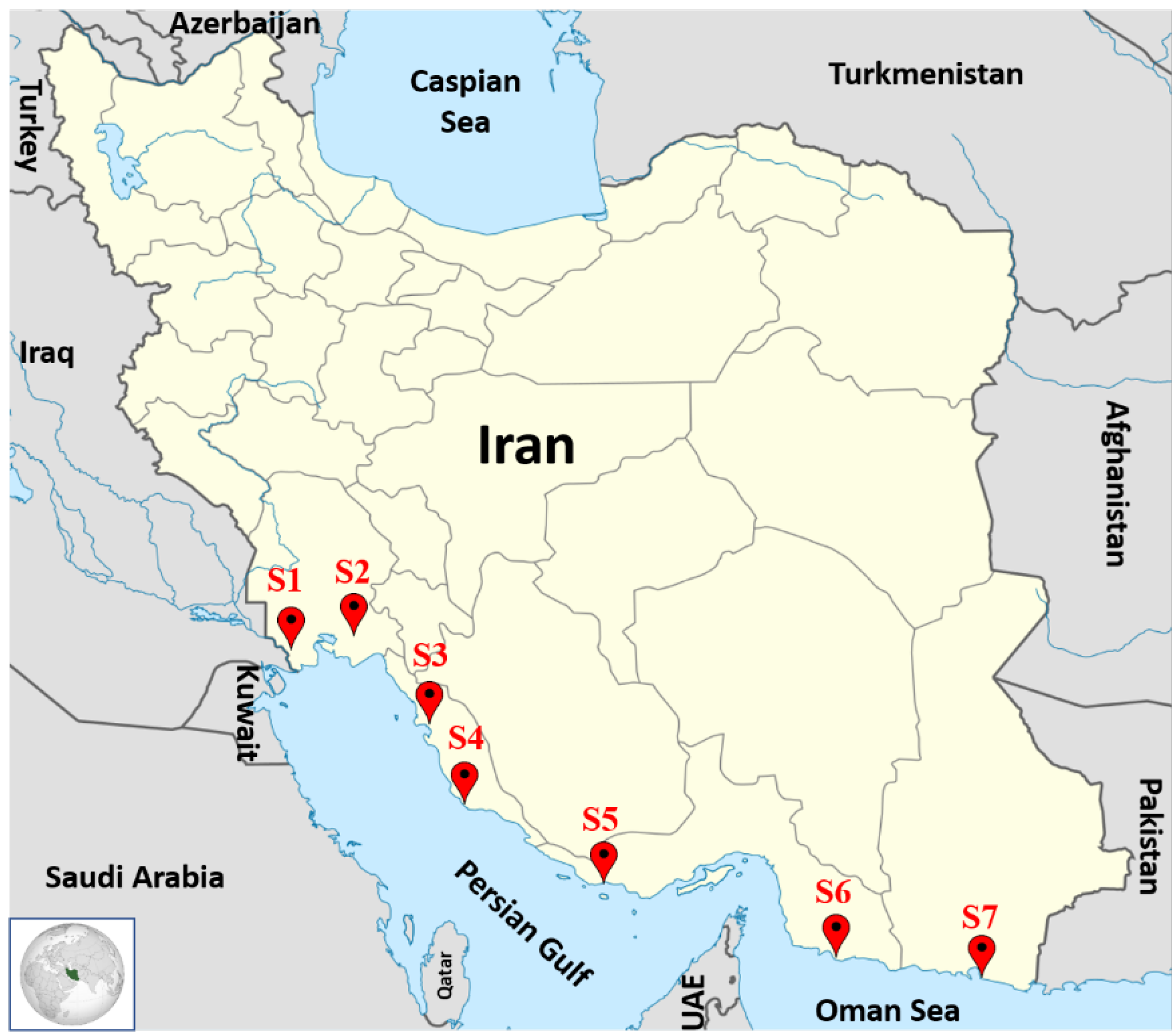
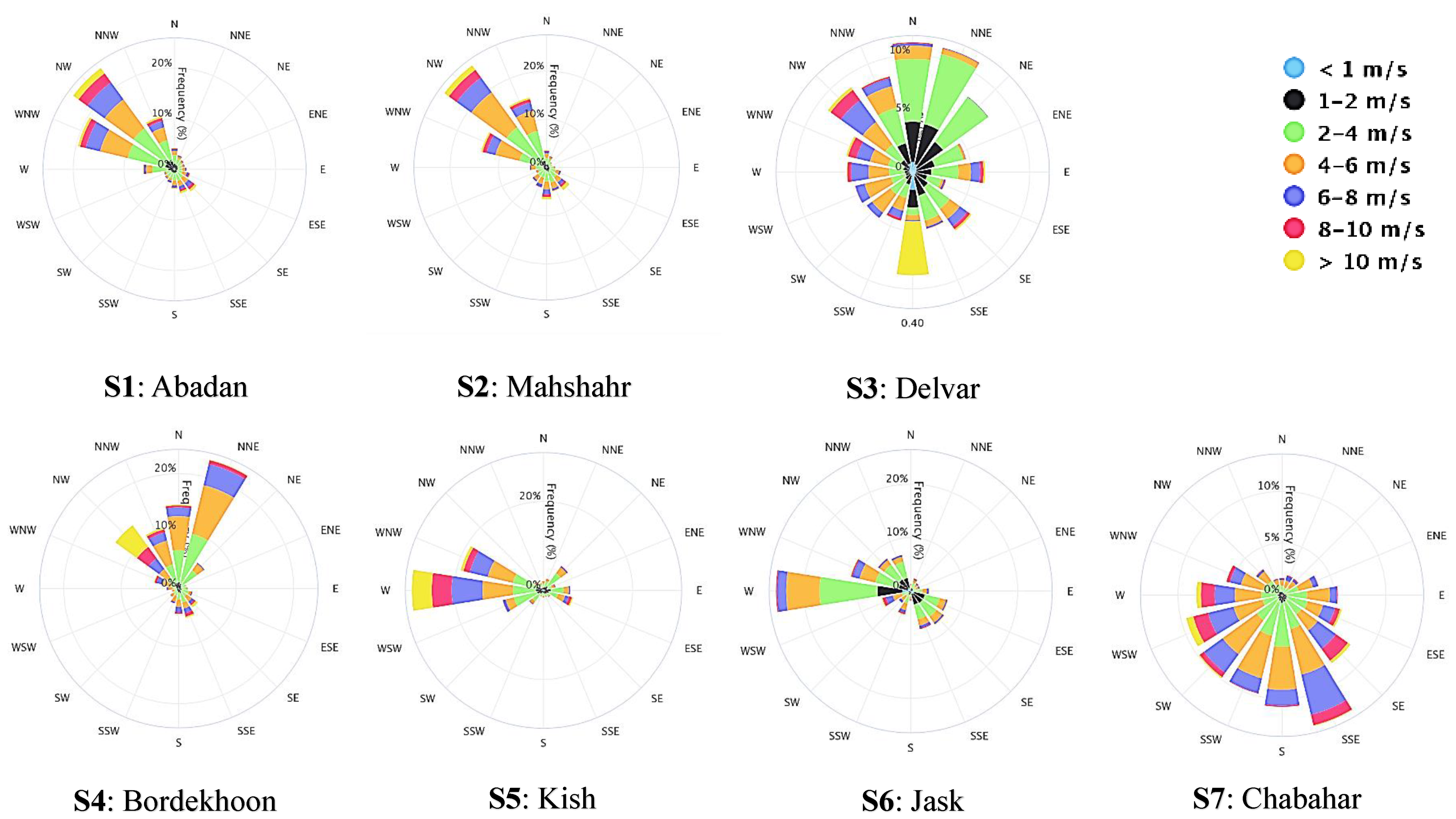
Wind power is mainly dependent on wind speed. Therefore, a reliable and accurate model for wind-speed data is a solid pavement for investigating wind energy potential. Numerous models have been used in the scientific literature (Section 3.1) and among them, Weibull is the most widely used distribution. However, all regions and their wind patterns cannot be modeled accurately by Weibull. There are numerous alternative distributions namely Gamma, Lognormal, Rayleigh, Nakagami, Gumbel, Burr, Generalized Extreme Value (GEV), Inverse Gaussian (IG), etc. [17,18]. Hence, in this study, different distributions (Weibull, Gamma, Rayleigh, GEV, IG, and Lognormal) are employed in order to find the most suitable model for wind-speed data based on the goodness of fit criteria.

There are many studies for Wind Resource Assessment (WRA) in Iran. In the past decade (from 2010 to 2019), 28 types of studies related to wind energy assessment in Iran gained more attention and citation.

Table 1. Comprehensive literature review for wind energy assessment.

Year	Ref.	Distribution (s)	Method of Estimation	Case Study Location	Coastal City?
2010	[26]	Weibull	Method of Moments	Tehran city	No
2011	[27]	Weibull	Empirical method	North and South Khorasan provinces	No
2011	[28]	Weibull	Empirical method	Semnan province	No
2011	[29]	Weibull	Method of Moments	Sharbabak city	No
2012	[30]	Weibull	Not mentioned	Abadan city	Yes
2013	[31]	Weibull	Empirical method	Kish and Jask regions	Yes
2013	[32]	Weibull	standard deviation method	Kerman province	No
2013	[33]	Weibull	standard deviation method	Aligoodarz city	No
2014	[20]	Weibull, Lognormal, Rayleigh, Logistic	graphical method, Maximum likelihood, Method of moments	Mahshahr city	Yes
2014	[34]	Weibull	standard deviation method	Mil-E Nader region	No
2014	[35]	Weibull	Empirical method	Chabahar, Kish and Salafchegan	Yes
2014	[36]	Weibull	Empirical method	Zahedan city	No
2015	[37]	Weibull	Method of Moments	Firouzkooh city	No
2015	[38]	Weibull	Method of Moments	Tabriz and Ardabil cities	No
2016	[22]	gamma, lognormal, Rayleigh, Weibull	Maximum likelihood, Method of moments	Bam, Bardsir, Arzuiyeh, Rafsanjan, Shahrbabak	No
2016	[39]	Weibull	Not mentioned	Kahnuj city	No
2016	[40]	Weibull	standard deviation method	Asaluyeh, Bordkhoon, Delvar, Haft-Chah	Yes
2016	[23]	Weibull	graphical method, Maximum likelihood, Method of moments	Gulf of Oman	Yes
2017	[41]	Weibull	maximum likelihood	Chabahar, Dehak and Dalgan	Yes (Chabahar)
2017	[42]	Weibull	Not mentioned	Fars province	No
2017	[3]	Weibull	standard deviation method	Zabol, Zahak, Zahedan and Mirjaveh cities	No
2018	[24]	Weibull	Standard deviation method, Empirical method of Lysen, Power density method	Nine central provinces	No
2018	[43]	Weibull	standard deviation method	provinces of East Azerbaijan, West Azerbaijan and Ardabil	No
2018	[25]	46 different functions	Not mentioned	Shurje region, Qazvin Province	No
2019	[44]	Weibull	Empirical method	Lotak and Shandol	No
2020	[45]	Weibull	Maximum-likelihood	Persian Gulf	No

presents the distribution function, method of estimation of parameters and the location in each study. Weibull was the most commonly used statistical distribution for describing wind speed data in such studies. In most of them (about 80%), the authors did not consider any further statistical investigations for selecting a suitable wind speed distribution and just used Weibull based on frequent usage while enjoying its simplicity. Moreover, there are a few studies of the coastal regions of Iran and most of them are for inland stations. Thus, a comparative study on the effectiveness of different wind speed distributions in the coastal stations is of great importance. In some of these studies performed statistical investigations to select the distribution or the method of estimation of parameters. For example, Mohammadi and Mostafaeipour used Weibull distribution for their study in Zarrineh city and calculated its parameters using two methods; standard deviation method and power density method [19]. They reported that the power density method is a better estimation method than the standard deviation method in monthly, seasonal, and yearly wind patterns.

In another study, Nedaei et al. compared the performance of four distribution functions (Weibull, Lognormal, Rayleigh, and Logistic) in Mahshahr station [20]. They found that the Weibull distribution is the best function to model wind data in Mahshahr, at two heights of 40 m and 10 m. They also used three different methods (graphical method, maximum likelihood, method of moments) for calculating Weibull parameters. The results show that the Graphical method at 10 m and method of moments at 40 m height are the best methods for calculating Weibull parameters in this city.

Furthermore, Alavi et al. investigated four different distribution functions (gamma, lognormal, Rayleigh, and Weibull) for five cities in Kerman province (Bam, Bardsir, Arzuiyeh, Rafsanjan, and Shahrbabak) [21]. They also used two methods for calculating Weibull parameters; maximum likelihood and method of moments. The experimental results show that the lognormal function produces better estimations for the actual data, while the Weibull model gives a better fit for the truncated wind speed data. They also concluded that calculating Weibull parameters using MLE perform perfectly well in comparison with MM estimations. Alavi et al. used eight PDFs (exponential, Weibull, gamma, lognormal, log-logistic, inverse-Gaussian, generalized extreme value, Nakagami) in their study and also computed the parameters using MLE for wind speed distribution in cities of Chabahar, Khaf, Lutak, Rafsanjan, and Zabol [22]. They found that Nakagami performs better than other distributions; however, because of the closed performance of the Nakagami and Weibull distributions, they finally proposed Weibull due to its flexibility and widely used. In [23], the graphical method, Maximum likelihood, and Method of moments were employed to estimate Weibull coefficients in a coastal area in the south of Iran in the Gulf of Oman. The authors asserted that the maximum likelihood method is the best algorithm to estimate Weibull parameters. Although the resulted output for the designated site is not considerable, more studies should be conducted for onshore wind power assessment in Iranian waters, the Persian Gulf and the Caspian Sea.

An alternative approach was proposed by Faghani et al. [24] used Weibull because of its popularity for WRA in 35 wind stations in nine provinces. Nevertheless, in order to calculate the Weibull parameters three different methods were used; including standard deviation method, empirical method of Lysen, power density method. Based on their investigations, authors concluded that the power density method is the most accurate method for extrapolating wind characteristics.

In a more comprehensive study, Nedaei et al. [25] fitted 46 different PDFs and suggested that the Wakeby distribution performs better than other distribution functions. They did not mention the method of estimating parameters. The distribution analysis is provided for only the ten most efficient PDFs, but details about the methodology for selecting these functions among others are not presented in the context of the paper.

2. Area of Interest

For the purpose of the current study, seven coastal stations are selected and investigated (Figure 2). The reason for selecting these stations is that in the first place, the Renewable Energy and Energy Efficiency Organization of Iran (SATBA) has provided public access to validated wind speed and direction data for several stations in Iran [46]. Some of these stations are nearshore and some are not. Since the case study has been on the southern coasts of Iran, which comprises four provinces: Sistan and Baluchestan, Hormozgan, Bushehr, and Khuzestan, in each of these provinces, the nearshore stations with available validated information are selected to cover the whole southern shoreline of Iran from east to west. Hence, these stations have been selected.

Table 2. Location and properties of studied wind data [46].

Station	Designate	Lat. (N)	Long. (E)	Data Period	Time Interval	Recorded Data	Data Statistics
							Mean	SD	Max.
Abadan	S1	30.447	48.306	2007–2009	10-min	90,656	4.35	2.51	19.76
Mahshahr	S2	30.579	49.086	2007–2009	10-min	91,923	4.44	2.41	21.46
Delvar	S3	28.835	51.046	2006–2008	10-min	72,186	3.40	2.14	15.92
Bordekhoon	S4	27.985	51.492	2006–2008	10-min	82,492	4.87	2.73	19.93
Kish	S5	26.553	53.910	2006–2008	10-min	81,217	4.59	2.81	22.38
Jask	S6	25.685	58.109	2006–2007	10-min	59,518	3.44	2.04	20.82
Chabahar	S7	25.328	60.663	2008–2009	10-min	73,296	4.97	2.14	15.41

shows some descriptive statistics of wind speed data in each of the seven stations including Latitude (Lat.), Longitude (Long.), data period, time interval, total recorded data, mean wind speed, standard deviation (Sd), maximum wind speed (Max.), locations and the data specifications for each station. According to Table 2, Chabahar (S7 station) has the highest mean wind speed with a value of 4.97 m/s, and therefore it has a great potential for harnessing wind energy.

One of the most effective factors in wind energy studies is wind direction distribution. Wind direction determines the optimal position of wind turbines and the whole array of wind farms. A wind rose is the best indicator for wind direction distribution. This graphical representative plays a vital role in choosing turbines and their alignments in the wind farm. Figure 3 shows wind roses of seven selected stations. As seen in these figures, dominant wind directions for stations S1 to S7 are NW, NW, N, NNE, W, W and SSE, respectively.

3. Analysis

A plausible resource assessment must be able to identify appropriate locations with strong, moderate, and weak winds. In the past, the assessment was performed through "wind deformed conifer trees". Here, trees and vegetation were the natural indicators for both wind speed and direction. By observing the local place for a long time, a rough idea about the wind richness of the place could be achieved [47]. Various techniques are used to show the effect of wind on trees in terms of numbers such as the Griggs-Putnam index [48]. A comprehensive review of these techniques was performed by Murthy et al. [49].

Although natural indicators are inexpensive, ubiquitous, simple, and conceivable to identify eligible locations, more detailed measurements must be performed to achieve better insight into station characteristics. With the advent of new technologies to measure wind properties, new horizons were broadened for the energy industry. To establish a meaningful analysis, a statistical analysis must be conducted. This procedure demands a time series record of wind speeds. Originally, measurement devices were used for airports across the world. Moreover, there are other technologies for on-station measurements. Therefore, the wind characteristics data pave the way for more precious and detailed researches in the energy industry.

Wind energy is the kinetic energy of air in motion. Total wind energy through an assumed surface area could be calculated through Equation (1):

$$E=\frac{1}{2}m{v}^2=\frac{1}{2}\left(Avt\rho \right)v^2=\frac{1}{2}At\rho v^3$$

(1)

$\rho$ is the air density, v is wind speed and $Avt$ combination is equal to the volume of air passing through the surface at the given time. Air density could be analyzed through statistical distributions to gain more concrete results [50]. In this study, air density is assumed to be constant. Therefore, the term $Avt\rho$ is equal to the mass of air flowing through assumed surface area (e.g., Rotor swept area of wind turbine). Power is energy per time unit; therefore, the output power of wind is [51]:

$$P=\frac{E}{t}=\frac{1}{2}A\rho v^3$$

(2)

Figure 4 shows the flowchart of this study. The initial step for any wind power feasibility study is the technical assessment. The vital part of the technical assessment is to study and analyze the statistical characteristics of wind speeds because the energy output of the field considerably depends on wind speeds and their patterns. Various studies asserted that the main part of the assessment is finding the PDF through wind speeds data as the main input into wind turbine design, station planning and operational plan [52]. After finding a suitable distribution, wind energy potential can be determined. The next step is to calculate the wind turbine capacity factor for all available options. If the capacity factor is less than 0.25, the selected turbine model is rejected. Else, it is selected as a potential option and annual energy output is calculated for it [53].

3.1. Wind Speed Distribution Models

In statistics, a unimodal distribution function refers to a continuous probability distribution that contains a single clear peak or the most frequent value. A diverse range of unimodal distribution functions was used in previous studies for modeling the PDF of wind speed including Weibull function, Gamma function, Rayleigh function, logistic function, Log-normal function, etc. Equations of these PDFs are listed in

Table 3. Investigated PDFs and their parameters.

Name	Probability Distribution Functions	Parameters
Weibull [57]	$f\left(v\right)=\frac{k}{c}.{\left(\frac{v}{c}\right)}^{k-1}.e^{-{\left(\frac{V}{c}\right)}^k}$	k: shape c: scale
Rayleigh [37]	$f\left(v\right)=\frac{2v}{c^2}.e^{-{\left(\frac{V}{c}\right)}^2}$	c: scale
Lognormal [27]	$f\left(v\right)=\frac{1}{c.v.\sqrt{2\pi }}exp\left[-\frac{1}{2}{\left(\frac{ln\left(v\right)-k}{c}\right)}^2\right]$	k: shape c: scale
Gamma [58]	$f\left(v\right)=\frac{v^{k-1}}{\mathsf{\Gamma }\left(k\right).c^k}exp\left(-\frac{v}{c}\right)$	k: shape c: scale
Inverse Gaussian [22]	$f\left(v\right)={\left(\frac{k}{2\pi v^3}\right)}^{\frac{1}{2}}.exp\left[-\frac{k{\left(v-c\right)}^2}{2v{c}^2}\right]$	k: shape c: scale
Generalized Extreme Value [2]	$f\left(v\right)=\frac{1}{\sigma }{\left(1+k\frac{v-\mu }{\sigma }\right)}^{-1-\frac{1}{k}}exp\left[-{\left(1+k\frac{v-\mu }{\sigma }\right)}^{\frac{-1}{k}}\right]$	k: shape $\sigma$: scale $\mu$: location

. Sometimes, wind speed data do not have a single clear peak. In these cases, multimodal probability distributions may provide a better fit for the data. Among these functions, the Weibull function is most used because of its simplicity and flexible parameters [28,40,54]. Although the Weibull is capable of analyzing very low wind speeds close to 0 m/s, it cannot represent the wind structure nature thoroughly [55]. One of the main limitations of the Weibull function is that it cannot accurately capture the effect of calm winds. A solution for this issue is to use some mixture functions like two-component mixture Weibull function (Weibull-Weibull) or truncated normal Weibull mixture (Normal-Weibull). This approach has been comprehensively studied by Tian et al. [56].

In more complex and accurate studies, air density could be related to the height from the ground or sea surface and model the relation between them for calculating Equation (2). Therefore, there must be two variations for estimating power output, wind speed, and air density. A Bivariate Probability Model (BPM) was proposed by Carta et al. to model wind speed and air density interactions in Spain [59].

As stated before, Weibull distribution is the most used PDF for the sake of statistical analysis of wind speed data. The first and prior stage to use Weibull distribution for investigating wind speed patterns, is to compute its distribution parameters. There are several methods in scientific contexts about this subject. Some of them are:

• Graphical method or Least squares algorithm [60]
• Maximum likelihood method (MLE) [61]
• Modified maximum likelihood method (MMLE) [61,62]
• Moments Method (MM) [61]
• Standard deviation method [63]
• Empirical method of Jestus [64]
• Empirical method of Lysen [65]
• Equivalent energy method [62]
• Energy pattern factor method (power density method) [66]
• WAsP method [49]

Three of the above-mentioned methods were most used in various studies: maximum likelihood [67,68,69,70], the empirical method [26,53,71,72], and the graphical method [73,74]. Moreover, the method of moments [64,75,76], energy pattern factor, equivalent energy method, and WAsP [61] are the other methods used for the calculation of Weibull coefficients. Different studies have compared the effectiveness of these methods. As mentioned in Shoaib et al.’s study, using the energy pattern factor method, maximum likelihood, and modified maximum likelihood results stated that maximum likelihood method is the most reliable method [77]. In one of the most comprehensive studies among different algorithms for determining Weibull coefficients, Rocha et al. attempted to evaluate and compare graphical, empirical, moment, Energy pattern factor, maximum likelihood, modified maximum likelihood, and equivalent energy methods in Brazil. It was observed that the equivalent energy method is the best method to calculate coefficients and graphical and energy pattern factor methods are the least effective ones to find coefficient values [63]. Solyali et al., used WAsP (Wind Atlas Analysis and Application), maximum likelihood, and graphical method algorithms [78]. Results indicate that the WAsP algorithm gains the highest correlation with the actual data. Allouhi et al. chose maximum likelihood, graphical, and WAsP methods to compute coefficients in Morocco [62]. Maximum likelihood presents the best fit with the actual data. Masseran, comprehensively compared Weibull, Rayleigh, Lognormal, Burr, Exponential, Inverse Gaussian, and Inverse Gamma in two stations in Malaysia [79]. Surprisingly, the Gamma function performed the best accuracy for the two stations, based on a combination of four goodness of fit indicators. It is worth mentioning here that there are uncertainties and variabilities related to renewable energy sources, e.g., wind. Therefore, it is important to address this challenge in feasibility studies. Using stochastic optimization approaches may be very helpful to address this challenge. For further information, references are recommended [80,81,82,83].

3.1.1. Wind Speed Extrapolation

The data record used in this study represents the wind specifications at the height of 10 m above ground. To find wind speed at the height of the turbine hub, power law has been used to convert wind speed. The wind speed fluctuations near the ground surface are referred to as wind shear. In the atmospheric surface boundary layer in which height does not exceed 150 m above the ground surface, the power-law rule is a reliable tool to extrapolate wind speeds at different heights [84]. It can be expressed by Equation (3):

$$\frac{V_H}{V_R}={\left(\frac{H}{R}\right)}^{\alpha }$$

(3)

where $V_H$ is the wind speed at height H, and $V_R$ is the reference wind speed at the reference height R which is 10m in the wind speed data, $\alpha$ coefficient is the Hellmann exponent, also named the wind shear coefficient (WSC). The WSC varies regarding ground level height, time of day, atmospheric stability, humidity, and roughness of terrain. The general values of WSCs are summarized in

Table 4. Wind Shear Coefficient (WSC) [85].

Terrain Type	WSC
Lake, ocean and smooth hard ground	0.10
Foot high grass on ground level	0.15
Tall crops, hedges, and shrubs	0.20
Wooded country	0.25
Small town with some trees and shrubs	0.30
City area with tall buildings	0.40

[85]. In this study, the WSC coefficient is assumed to be equal to 0.2 due to a lack of reliable data for the stations.

3.1.2. Goodness of Fit Tests

Now it is time to assess the goodness of fitted PDFs for modeling the wind speed probability distribution. There are various Goodness-of-Fit (GoF) tests to assess the quality of fitted distributions. The coefficient of determination (R²) is used to measure the linear relationship between the observed and predicted probabilities. Additionally, root-mean-square error (RMSE) is used to show the level of concentration of data around the fitted distribution. Moreover, because of using the MLE method for parameter estimation Akaike information criterion (AIC) and Bayesian information criterion (BIC) is used to assess the accuracy of the fitted distribution.

Table 5. Goodness-of-Fit (GoF) tests in this study.

Indicator	Formula	Parameters
R2	$R^2=1-\frac{{\sum }_{i=1}^n{\left(y_i-y_{ic}\right)}^2}{{\sum }_{i=1}^n{\left(y_i-\overline{y}\right)}^2}$	$y_i$: Observed data $y_{ic}$: fitted data n: Number of data samples.
RMSE	$RMSE={\left[\frac{1}{n}{\sum }_{i=1}^n{\left(y_i-y_{ic}\right)}^2\right]}^{\frac{1}{2}}$	$y_i$: Observed data $y_{ic}$: fitted data n: number of data samples
AIC	$AIC=-2log\left(L\right)+2k$	L: likelihood k: number of parameters
BIC	$BIC=-2log\left(L\right)+klogn$	L: likelihood k: number of parameters n: number of data samples

presents the formulae and definitions of parameters for each of these four statistical indicators. Lower values for RMSE, AIC, and BIC indicate higher goodness of fit, while on the contrary, a larger value for R² shows better effectiveness of the fitted distribution.

3.2. Wind Power and Energy Density

After calculating Weibull distribution function parameters, the next crucial step will determine wind power density through using Weibull distribution parameters. Wind power density is one of the most meaningful indicators to depict how powerful the winds are in a region within the defined time period. By contemplating the wind power density, quantification of the potential wind energy electricity is possible. Wind power is directly related to the area of the turbine (i.e., swept area) and the cube of wind velocity at the station. Wind power can be calculated as Equation (4):

$$P_w=\frac{1}{2}\rho A{\int }_0^{\infty }{v}^{3}f\left(v\right)dv$$

(4)

Note that in the above equation, the area of turbine and air density is considered as constant values. The more tangible indicator for wind energy is the power per unit area. It can be written as Equation (5):

$$P_d={\int }_0^{\infty }\frac{1}{2}\rho v^{3}f\left(v\right)dv$$

(5)

The wind power density using Weibull distribution for wind speed patterns will be stated as [53,62]:

$$P_d=\frac{1}{2}\rho c^3\mathsf{\Gamma }\left(1+\frac{3}{k}\right)$$

(6)

While using the Rayleigh probability distribution function as a distribution of wind speeds, the wind power density function will be written as [86]:

$$P_d=\frac{3}{\pi }\rho c^3{\left(\frac{\pi }{4}\right)}^{\frac{3}{2}}$$

(7)

For another distributions, there are not any analytic answers for the integral in Equation (4). Therefore, the wind power density is calculated using numerical integration.

There is a reliable classification for every station based on National Renewable Energy Laboratory (NREL) to determine the relative wind power potential. This classification is based on observed and recorded wind speeds at the height of 50 m. The wind power classification is given in

Table 6. NREL wind power classifications.

Wind Power Class	Power Density (W/m2)	Description
1	0–200	Unsuitable for any wind applications
2	200–300	Suitable for Stand-alone
3	300–400	Good
4	400–500	Good
5	500–600	Excellent
6	600–800	Outstanding
7	800–2000	Superb

[87].

Wind energy density is the amount of energy produced for any arbitrary period of time. It can be written as Equation (8):

$$P_d=\frac{E_d}{t}$$

(8)

3.3. Capacity Factor

The capacity factor (C_f) of a wind turbine is an indicator that defines the output viability of a wind turbine at a selected station. It determines the ratio of average power yield to the rated power of the turbine. C_f is one the most reliable measures for choosing wind turbine because it inherently shows the performance of the wind turbine. C_f can be expressed as [53]:

$$C_f=\frac{P_{avg}}{P_r}=\frac{Netannualenergyproduction{}_{\left(MWh\right)}}{Installedpower{}_{\left(MW\right)}.Annualhours}$$

(9)

$P_r$ Represents the power output of wind turbine when the turbine runs as its rated power all the time in one year. Needless to say, the capacity factor is always less than 1. The $P_{avg}$ can be expressed as [62]:

$$P_{avg}={\int }_{V_{cut-in}}^{V_{cut-out}}P\left(v\right).f\left(v\right)dv$$

(10)

where $f\left(v\right)$ is the probability distribution of wind speed and $P\left(v\right)$ is the power curve of wind turbines. The cut-in wind speed is the minimum wind speed at which the turbine blades overcome the friction and begin to rotate. The cut-out wind speed is the speed at which turbine blades stopped rotating to prevent probable damages from high winds. It is notable that not all turbines have a well-defined cut-out speed. The schematic concept of power curve for a wind turbine is presented in Figure 5.

For pitch controlled turbines, the generated power from wind turbines can be estimated from the power curve as [53]:

$$P_{avg}=\left\{\begin{array}{cc}{P}_r\ast c\left(v\right)\hfill & \hfill \left(v_{\mathrm{cut}-\mathrm{in}}\le v_i\le v_r\right)\\ P_r\hfill & \hfill \left(v_r\le v_i\le v_{\mathrm{cut}-\mathrm{off}}\right)\\ 0\hfill & \hfill \left(v_i\le v_{\mathrm{cut}-\mathrm{in}}\mathrm{or}{v}_i\ge v_{\mathrm{cut}-\mathrm{off}}\right)\end{array}\right.$$

(11)

The function $c\left(v\right)$ denotes the wind turbine’s output power in the interval between cut-in and cut-off speeds. In recent years, several studies have been conducted by scholars aiming to approximate this function [53,89,90]. The six most widely used functions for this purpose are listed as follows from Equations (12)–(17):

$$c_1\left(v\right)=\frac{v-v_i}{v_r-v_i}$$

(12)

$$c_2\left(v\right)=\frac{{\left(v-v_i\right)}^2}{{\left(v_r-v_i\right)}^2}$$

(13)

$$c_3\left(v\right)=\frac{{\left(v-v_i\right)}^3}{{\left(v_r-v_i\right)}^3}$$

(14)

$$c_4\left(v\right)=\frac{v^2-v_i^2}{v_r^2-v_i^2}$$

(15)

$$c_5\left(v\right)=\frac{v^3-v_i^3}{v_r^3-v_i^3}$$

(16)

$$c_6\left(v\right)=\frac{v^3}{v_r^3}$$

(17)

The simultaneous power output of wind turbines in a wind farm is not the same because of the spatial distribution of turbines and the unpredictable and stochastic nature of wind speed distribution. Therefore, a more complicated approach is required to obtain the power output. Based on Wang et al., the average of the above six functions is used for estimating the capacity factor [52].

$$C_f=\frac{P_{avg}}{P_r}=\left[{\int }_{v_{cut-in}}^{v_r}c\left(v\right)f\left(v\right)dv+{\int }_{v_r}^{v_{cut-off}}f\left(v\right)dv\right]$$

(18)

Therefore, the wind turbine will work within the speed period between cut-in and cut-off speeds.

3.4. Availability Factor

According to Section 2, wind turbine will work within the wind speed interval between the cut-in and cut-off speeds. Thus, the availability factor of a wind turbine can be expressed as Equation (19):

$$AF={\int }_{v_{cut-in}}^{v_{cut-off}}f\left(v\right)dv$$

(19)

where $f\left(v\right)$ is the wind speed probability distribution function.

4. Results and Discussion

4.1. Analysis of Distribution Functions

Six different probability distributions, which are most widely used in the scientific literature, are fitted to the wind speed data of each station. The Rayleigh PDF as a one-parameter function, Gamma, Log-normal, Weibull and Inverse Gaussian as two-parameter functions and finally, GEV as a three-parameter function are used for this purpose. MLE is used to estimate PDF parameters, since it is more efficient than other estimation methods, and generates a lower mean squared error [22]. The estimated parameters for each region are reported in

Table 7. Estimated parameters of probability distribution functions of the stations at height of 10 m.

Station	Distribution
	Weibull	Gamma	Lognormal	GEV	Rayleigh	IG
S1	k = 1.837, c = 4.910	k = 3.019, c = 1.440	LL = 1.295, LS = 0.625	k = 0.0702, sigma = 1.825, mu = 3.157	c = 3.548	k = 8.798, c = 4.347
S2	k = 1.942, c = 5.012	k = 3.390, c = 1.309	LL = 1.33541, LS = 0.607406	k = 0.032, sigma = 1.791, mu = 3.345	c = 3.569	k = 4.919, c = 4.438
S3	k = 1.677, c = 3.821	k = 2.540, c = 1.338	LL = 1.014, LS = 0.694	k = 0.1432, sigma = 1.454, mu = 2.334	c = 2.841	k = 4.495, c = 3.399
S4	k = 1.899, c = 5.508	k = 3.392, c = 1.436	LL = 1.428, LS = 0.659	k = 0.077, sigma = 1.928, mu = 3.597	c = 3.946	k = 11.435, c = 4.869
S5	k = 1.720, c = 5.164	k = 2.620, c = 1.752	LL = 1.321, LS = 0.690	k = 0.093, sigma = 1.997, mu = 3.232	c = 3.805	k = 5.579, c = 4.589
S6	k = 1.755, c = 3.862	k = 2.625, c = 1.310	LL = 1.032, LS = 0.723	k = 0.042, sigma = 1.522, mu = 2.492	c = 2.826	k = 1.955, c = 3.438
S7	k = 2.474, c = 5.605	k = 4.780, c = 1.040	LL = 1.495, LS = 0.503	k = -0.124, sigma = 1.908, mu = 4.075	c = 3.827	k = 14.317, c = 4.971

. Note that the parameters are calculated from wind data at 10 m above the ground.

The wind speed distribution diagrams (PDF plots) for seven selected stations are shown in Figure 6. The horizontal axis of these diagrams shows the range of wind speed and the vertical axis is the probability density. It varies from zero to the highest possible value for each curve. As seen in figures, all distributions are skewed to the right (i.e., positive Skewness), and therefore, the mean of wind speeds is bigger than the mode and median of data.

Four different GoF indicators are calculated for these functions and the results are reported in

Table 8. Comparison between six distribution functions in terms of four GoF indicators.

Station	Distribution Function	R2		RMSE		AIC		BIC
		Value	Rank	Value	Rank	Value	Rank	Value	Rank
S1	Weibull	0.953	4	0.045	4	404,569	3	404,551	3
	Gamma	0.989	1	0.026	1	401,817	1	401,798	1
	Lognormal	0.976	2	0.397	3	406,898	5	406,879	4
	GEV	0.972	3	0.345	2	402,987	2	402,959	2
	Rayleigh	0.943	5	0.049	5	405,758	4	405,766	5
	IG	0.921	6	0.058	6	412,268	6	412,276	6
S2	Weibull	0.924	3	0.061	4	406,040	3	406,059	3
	Gamma	0.959	2	0.045	2	403,145	2	403,164	2
	Lognormal	0.917	4	0.064	5	414,720	5	414,739	5
	GEV	0.988	1	0.029	1	400,500	1	400,528	1
	Rayleigh	0.924	3	0.059	3	406,188	4	406,196	4
	IG	0.516	5	0.15	6	406,188	4	406,196	4
S3	Weibull	0.913	4	0.068	3	295,197	3	295,215	3
	Gamma	0.969	1	0.049	2	293,315	1	293,334	1
	Lognormal	0.955	2	0.041	1	298,399	4	298,418	4
	GEV	0.929	3	0.076	4	294,194	2	294,222	2
	Rayleigh	0.857	6	0.09	6	299,472	5	299,479	5
	IG	0.877	5	0.084	5	315,908	6	315,916	6
S4	Weibull	0.924	4	0.055	4	381,906	5	381,888	5
	Gamma	0.976	2	0.031	2	377,063	2	377,082	2
	Lognormal	0.963	3	0.039	3	380,270	4	380,289	4
	GEV	0.992	1	0.023	1	376,076	1	376,104	1
	Rayleigh	0.924	4	0.055	4	377,578	3	377,586	3
	IG	0.918	5	0.057	5	377,578	3	377,586	3
S5	Weibull	0.967	4	0.035	3	378,525	3	378,544	3
	Gamma	0.993	1	0.016	1	377,071	1	377,089	1
	Lognormal	0.974	2	0.032	2	384,730	5	384,748	5
	GEV	0.973	3	0.04	4	378,108	2	378,136	2
	Rayleigh	0.925	5	0.052	5	382,014	4	382,022	4
	IG	0.806	6	0.083	6	412,722	6	412,729	6
S6	Weibull	0.975	3	0.038	3	241,574	2	241,592	2
	Gamma	0.985	2	0.028	1	241,851	3	241,869	3
	Lognormal	0.937	5	0.06	5	253,252	5	253,270	5
	GEV	0.986	1	0.035	2	240,873	1	240,900	1
	Rayleigh	0.958	4	0.048	4	243,486	4	243,493	4
	IG	0.246	6	0.205	6	313,354	6	313,361	6
S7	Weibull	0.994	1	0.015	1	315,837	3	315,856	2
	Gamma	0.984	4	0.024	4	317,647	2	317,666	3
	Lognormal	0.923	6	0.053	6	326,363	5	32,632	5
	GEV	0.969	5	0.033	5	315,762	1	315,789	1
	Rayleigh	0.99	3	0.021	3	320,866	4	320,874	4
	IG	0.991	2	0.02	2	341,748	6	341,756	6

. Note that lower RMSE, AIC, and BIC show better fitness. On the other hand, higher R² shows a better correlation between observed data and fitted distribution. Note that different GoF indicators can yield different results. For example, in the S3 station, Gamma performs better in terms of R², whereas Lognormal performs better in terms of RMSE. This paper assigns R² a greater weight for the assessment and selects it as the first reference index. Results show that Gamma is the best distribution for S1, S3, S5, and GEV has the best fit for S2, S4, and S6. Weibull is only suitable for S7. Results show that R² values for Weibull distribution are 1 to 7 % lower than that of the best distribution in stations S1 to S6.

As seen above, one cannot use Weibull distribution for all stations without further investigations. Nevertheless, for engineering applications, it is valuable to propose an effective function that has the best performance to be used for a specific geographical location. The results show that Gamma and GEV are the most effective function for the southern coasts of Iran since they have the best statistical performance. However, Gamma has two parameters, whereas GEV has three parameters. Therefore, Gamma is selected as the effective function for the southern coasts because of its more simplicity. It should be mentioned that by increasing the length of the data and the number of distributions and even the fitting method, one can clearly expect different fitted distributions. This originates from the nature of statistical research. Considerably more work will need to generalize the obtained distributions and to propose them as the optimal distributions for the selected sites.

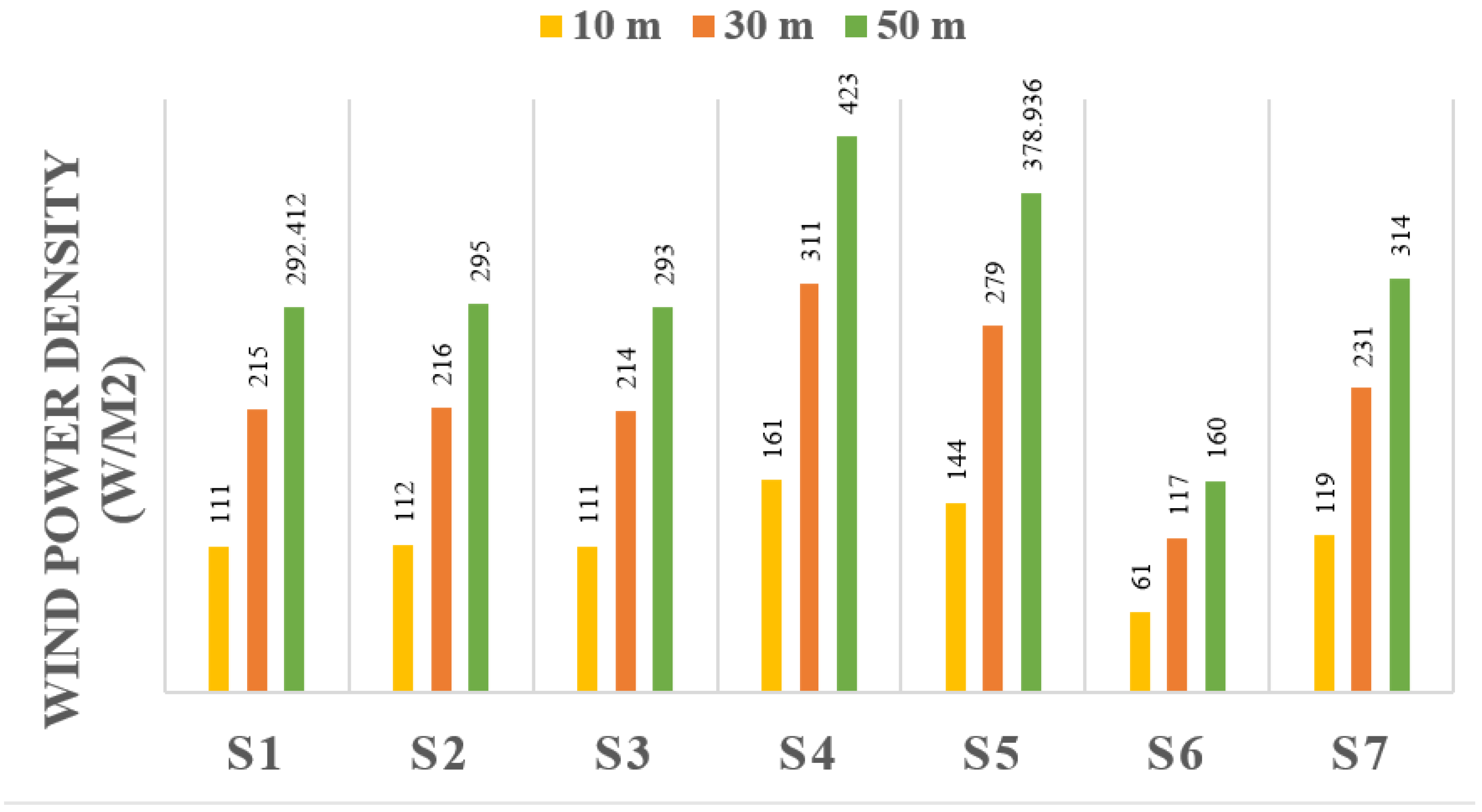
4.2. Analysis of Wind Power and Energy Density

The wind power density for each station is determined using the best-fitted probability distribution at 10, 30 and 50 m above the ground. Once the wind power density is calculated, wind energy density can be found. In this study, wind energy density is computed for one year. The results are gathered in

Table 9. Estimated wind power density and wind energy density and classification of the stations for the wind power based on NREL.

Station	PDF	WPD (W/m2)	WED ($\frac{\mathit{kWh}}{{\mathit{m}}^2}/\mathit{year}$ )	Class
		10 m	30 m	50 m	10 m	30 m	50 m
S1	Gamma	111	215	292	972	1883	2562	2
S2	GEV	112	216	295	981	1892	2584	2
S3	Gamma	111	214	293	972	1875	2567	2
S4	GEV	161	311	423	1410	2724	3705	4
S5	Gamma	144	279	379	1261	2444	3319	3
S6	GEV	61	117	160	534	1025	1402	1
S7	Weibull	119	231	314	1042	2024	2751	3

. For the sake of comparison, wind powers for each height across the stations are shown in Figure 7.

4.3. Wind Turbine Selection

Fifteen wind turbines with hub heights ranging 20–100 m and rated powers ranging 0.055–4.2 MW are exploited for assessing wind performance. This range of wind turbine power classes could be useful in the next steps of economic and feasibility analysis for establishing wind farms. Wind turbines characteristics are listed in

Table 10. Characteristics of wind turbines used in the study [91].

Turbine Model	Name	Rated Power Output (MW)	Hub Height (m)	Cut-in Wind Speed (m/s)	Rated Wind Speed (m/s)	Cut-Out Wind Speed (m/s)	Swept Area (m2)
Vestas V15	T1	0.055	20	4	12.5	25	176
AIRCON 10 S	T2	0.0098	30	3.5	11	25	39.6
Enercon E-12	T3	0.03	30	3	11	35	113
Enercon E-44	T4	0.9	45	3	16.5	34	1521
Enercon E-30	T5	0.3	50	2.5	13.5	25	707
Goldwind S43/600	T6	0.6	50	3	14	25	1452
Vestas V52	T7	0.85	55	4	14	25	2124
Goldwind S50/750	T8	0.75	60	3.5	14.5	25	1964
Nordex N54	T9	1	60	3.5	14	25	2290
Suzlon S.33-350	T10	0.35	70	3.5	14	25	876.1
United Power UP2000-97	T11	2	80	3	10.1	25	7390
Goldwind GW 62/1200	T12	1.2	85	3	12.5	25	3000
Envision EN106-1.8	T13	1.8	90	3	9.5	20	8825
General Electric GE 1.6-100	T14	1.6	100	3.5	11	25	7854
Senvion 4.2M118	T15	4.2	100	3	12.5	22	10,936

.

To evaluate the energy output of each turbine, wind speed distribution parameters have been calculated at the hub-height. Consequently, wind turbine capacity factor and availability factor are determined using Equations (18) and (19), respectively.

For cost-effective investment in the wind energy sector, it is asserted that the capacity factor of wind turbines should be between 0.25–0.45 to be economically efficient and feasible [92]. According to Ayodele et al., any wind turbine with a capacity factor lower than 0.25 will not be suitable to be integrated into the grid [53]. Estimated capacity factors for all wind turbines are listed in

Table 11. Annual energy output (MWh) for selected turbines on the stations.

Station	Turbine	T2	T3	T11	T12	T13	T14	T15
S1	Capacity factor	-	-	0.360	0.258	0.401	0.330	0.278
	Annual energy output (MWh)	-	-	6312	2710	6315	4630	10223
S2	Capacity factor	-	-	0.367	0.258	0.412	0.335	0.279
	Annual energy output (MWh)	-	-	6432	2716	6489	4691	10273
S4	Capacity factor	-	0.260	0.416	0.302	0.455	0.382	0.320
	Annual energy output (MWh)	-	68	7282	3172	7168	5358	11783
S5	Capacity factor	-	-	0.388	0.298	0.421	0.359	0.304
	Annual energy output (MWh)	-	-	6796	3136	6631	5027	11170
S7	Capacity factor	0.264	0.279	0.481	0.336	0.540	0.444	0.368
	Annual energy output (MWh)	23	73	8423	3530	8517	6218	13,538

.

Capacity factors higher than 0.25 could be plausible for a wind turbine [53]. Based on this, in Abadan, T11 to T15 are suitable for wind energy production. The table reveals that in Mahshahr again T11 to T15 are reliable for energy production. After that, in Delvar station, there is not any capacity factor higher than 0.25 but, T13 has the highest capacity factor. In Bordekhoon, one of the most suitable stations, T3 and T11 to T15 are suitable choices. Kish, the most important island of the Persian Gulf for tourism, again T11 to T15 are good for wind energy production. Jask has not any acceptable capacity factors due to poor wind power density. Eventually, in Chabahar station, T2, T3, and T11 to T15 are acceptable wind turbines with significant capacity factors.

The availability factor for each wind turbine in each station has been calculated and shown in

Table 12. Estimated Availability factor of wind turbines for each turbine across the seven stations.

	S1	S2	S3	S4	S5	S6	S7
T1	0.570	0.604	0.366	0.653	0.585	0.410	0.735
T2	0.695	0.741	0.487	0.778	0.698	0.542	0.834
T3	0.733	0.816	0.577	0.847	0.766	0.630	0.884
T4	0.802	0.848	0.622	0.875	0.797	0.672	0.904
T5	0.809	0.907	0.724	0.924	0.860	0.765	0.941
T6	0.731	0.855	0.630	0.879	0.803	0.683	0.908
T7	0.687	0.733	0.478	0.771	0.691	0.535	0.830
T8	0.761	0.809	0.564	0.838	0.758	0.621	0.879
T9	0.761	0.081	0.564	0.838	0.758	0.638	0.879
T10	0.774	0.822	0.581	0.849	0.770	0.727	0.888
T11	0.842	0.884	0.678	0.903	0.833	0.726	0.926
T12	0.731	0.884	0.678	0.903	0.839	0.730	0.926
T13	0.844	0.884	0.682	0.897	0.829	0.736	0.930
T14	0.803	0.848	0.619	0.872	0.795	0.675	0.905
T15	0.731	0.893	0.696	0.906	0.840	0.746	0.934

. As shown in Table 12, Bordekhoon and Chabahar stations have the greatest availability factors among stations. This fact could be realized from their greater wind power density and their higher average wind speed. After them, Kish, Mahshahr, and Abadan have the greatest availability factors. Jask and Delvar are the least in availability factors due to their poor wind power density. Among wind turbines, T5 has the greatest average of availability factor because it has the least cut-in speed and this turbine cover the wider range of applicable wind speeds.

4.4. Comparison with Previous Studies

In Abadan (S1), there is one similar study for wind energy potential [30]. The data used in this study is the same as in the current research. Weibull distribution was deployed for characterizing wind speed patterns. Nevertheless, the Weibull distribution ranked fourth among distributions used in this study. The best PDF for S1 is Gamma distribution. A precise comparison for the goodness of fit is not possible because it was not reported in that paper.

For Mahshahr city (S2), Nedaei et al. studied data with 19 months duration for the region and used Weibull, Rayleigh, and Lognormal distributions [20]. Reported R² in that paper are 0.923, 0.910, and 0.901, respectively, which are consistent with R² of the current study with the values 0.926, 0.924, and 0.917. Furthermore, in the current study, GEV has the best performance in terms of R² value and has R² = 0.988.

In Delvar city (S3), Dabbaghiyan et al. studied wind speed data for 2011 [40]. They deployed Weibull distribution for wind speed, but R² is not published. While, in this study, Gamma function is selected for this location with R² = 0.969.

Two studies were conducted on Kish Island (S5). Nedaei studied wind data between 2006 and 2007 and also selected Weibull distribution [31]. R² for Weibull distribution was 0.986, while Gamma distribution has the highest R² equal to 0.993 in the current study. Although R² is slightly increased, different data sources should be considered. Another study in the region is performed by Mohammadi et al. [35] based on long-term data from 2002 to 2009. Again, Weibull distribution opted. R² was not calculated. Wind power density at the height of 10m reported 111 W/m², while this research calculated 144 W/m² using Gamma density function with R² equal to 0.993.

In the Jask station (S6), Nedaei studied wind power density using data from 2006 to 2007 and Weibull distribution [31]. R² reported 0.9782 while in current research GEV function was the most suitable for the region with R² = 0.986. Weibull distribution ranked third among six PDFs with R² = 0.975, which is in line with the previous study.

Chabahar (S7) is the most studied location with three studies. Minaeian et al. studied wind speed data for 2007 and used Weibull distribution but R² was not reported [41]. Mohammadi et al. studied data from 2002 to 2009 and used Weibull distribution [35]. Again, R² was not announced. Wind power density at the height of 10 m is calculated 111 W/m² while in the current study, using Gamma function, wind power density is determined as 119 W/m² which is slightly higher. This distinction might cause due to different wind speed data and distribution used. Moreover, Alavi et al. studied the station with data from 2008 to 2009. They conducted analysis using Weibull, Gamma, Lognormal, and GEV functions with R² = 0.999, 0.999, 0.998, and 0.999 respectively which are significantly high. Additionally, Nakagami distribution function yielded the best fitness with R² = 0.9999. Accordingly, in the current study, R² for those distributions are 0.994, 0.984, 0.923, and 0.969, respectively. Apart from Nakagami distribution, Weibull shows the best fitness in both studies and R² of the two analyses are approximately equal. The negligible difference might occur because of different data. It should be noted that this region is very important in the development programs of Iran and therefore has great potential for the construction of coastal and offshore structures [93,94].

As mentioned above, current research enhanced goodness of fit for wind speed data according to R² in comparison with previous studies. Moreover, in other sections of the analysis, a more precise approach is conducted to compute capacity factors. Additionally, to increase the practicality of the article, a broad range of wind turbines are considered to analysis to obtain a more concrete insight toward wind energy capacity in the south coastal zone of Iran.

5. Conclusions

This paper presented a comprehensive and step-by-step methodology for the wind energy assessment along with a case study in seven different stations covering the southern coastal borders of Iran. Moreover, an extensive literature review is conducted to gain insight into the concept of wind energy assessment and efforts made in this field, their methodologies, and locations. The majority of previous studies in Iran used the Weibull function in order to estimate wind speed patterns in the selected area. Here, six different probability distribution functions ranging from one to three parameters were exploited in order to find the best fitness to the wind speed data. Furthermore, they exploited only a single function for determining the capacity factor of wind turbines. This study has shown that although the Weibull PDF is the most well-known function as wind speed distribution, in the area of interest, Gamma, GEV, and lognormal functions have better correlations with observed data. The second major finding was that based on the distribution ranks, the Gamma function is considered as the most suitable distribution at the initial step of wind power assessment in the southern coasts of Iran. Additionally, the annual wind power density and energy output are determined for three heights above the ground surface. Based on power densities, Bordekhoon, Kish, and Chabahar are more suitable for harnessing wind energy. Jask has the least power density and Abadan, Mahshahr, and Delvar are suitable for stand-alone wind power facilities. Moreover, the capacity factor of wind turbines is calculated through six different functions and the average of these six functions is used as a final capacity factor value to have more reliable results. This provides an accurate evaluation of wind energy capacity. To analyze practical aspects of the current study, fifteen wind turbines with hub heights ranging 20–100 m and rated powers ranging 0.055–4.2 MW are exploited for assessing wind performance. The achieved results show that as capacity factor increases with the hub height of wind turbine, T11 to T15 are the best wind turbines due to their capacity factors. The present study is the primary comprehensive practical assessment of wind energy along with assessing different actual turbine models.

Further research can be undertaken to explore economic aspects of implementing wind energy farms in the southern coasts of Iran by employing the levelized cost of energy (LCOE). This approach is used in similar research by the authors [10] for the tidal current energy in this area.

References

1. Amini, E.; Golbaz, D.; Amini, F.; Majidi Nezhad, M.; Neshat, M.; Astiaso Garcia, D. A parametric study of wave energy converter layouts in real wave models. Energies 2020, 13, 6095. [Google Scholar] [CrossRef]
2. Shukla, R.K.; Trivedi, M.; Kumar, M. On the proficient use of GEV distribution: A case study of subtropical monsoon region in India. arXiv 2012, arXiv:1203.0642. [Google Scholar]
3. Fazelpour, F.; Markarian, E.; Soltani, N. Wind energy potential and economic assessment of four locations in Sistan and Balouchestan province in Iran. Renew. Energy 2017, 109, 646–667. [Google Scholar] [CrossRef]
4. GWEC. Global Wind Capacity Forecast to Hit 800 GW by 2021; GWEC: Brussels, Belgium, 2021; in press. [Google Scholar]
5. IRENA. Global Energy Transformation: A Roadmap to 2050; International Renewable Energy Agency: Abu Dhabi, United Arab Emirates, 2018. [Google Scholar]
6. Heravi, G.; Salehi, M.M.; Rostami, M. Identifying cost-optimal options for a typical residential nearly zero energy building’s design in developing countries. Clean Technol. Environ. Policy 2020, 22, 2107–2128. [Google Scholar] [CrossRef]
7. Radfar, S.; Panahi, R. Economic Analysis of Developing Tidal Stream Energy Farms in the South Coasts of Iran. Iran. J. Mar. Sci. Technol. 2017, 21, 41–47. [Google Scholar]
8. Amini, E.; Golbaz, D.; Asadi, R.; Nasiri, M.; Ceylan, O.; Majidi Nezhad, M.; Neshat, M. A Comparative Study of Metaheuristic Algorithms for Wave Energy Converter Power Take-Off Optimisation: A Case Study for Eastern Australia. J. Mar. Sci. Eng. 2021, 9, 490. [Google Scholar] [CrossRef]
9. Neshat, M.; Sergiienko, N.Y.; Amini, E.; Majidi Nezhad, M.; Astiaso Garcia, D.; Alexander, B.; Wagner, M. A New Bi-Level Optimisation Framework for Optimising a Multi-Mode Wave Energy Converter Design: A Case Study for the Marettimo Island, Mediterranean Sea. Energies 2020, 13, 5498. [Google Scholar] [CrossRef]
10. Radfar, S.; Panahi, R.; Javaherchi, T.; Filom, S.; Mazyaki, A.R. A comprehensive insight into tidal stream energy farms in Iran. Renew. Sustain. Energy Rev. 2017, 79, 323–338. [Google Scholar] [CrossRef]
11. Mills, R. The Politics of Low-Carbon Energy in Iran and Iraq. In Low Carbon Energy in the Middle East and North Africa; Springer: Berlin/Heidelberg, Germany, 2021; pp. 19–56. [Google Scholar]
12. Amiri, A.; Panahi, R.; Radfar, S. Parametric study of two-body floating-point wave absorber. J. Mar. Sci. Appl. 2016, 15, 41–49. [Google Scholar] [CrossRef]
13. Wheeler, E.; Desai, M. Iran’s Renewable Energy Potential; Middle East Institute: Washington, DC, USA, 2016. [Google Scholar]
14. Aien, M.; Mahdavi, O. On the Way of Policy Making to Reduce the Reliance of Fossil Fuels: Case Study of Iran. Sustainability 2020, 12, 10606. [Google Scholar] [CrossRef]
15. Karaminia, G.; Tavanpourpaveh, M.; Amini, F. Atlas of Energy, 3rd ed.; National Cartographic Center: Tehran, Iran, 2014. [Google Scholar]
16. Renewable Energy and Energy Efficiency Organization. Renewable Atlas Coordinates and Current Status of the Stations; Renewable Energy and Energy Efficiency Organization: Abu Dhabi, United Arab Emirates, 2020. [Google Scholar]
17. Korzeniowski, A.; Ghorbani, N. Put Options with Linear Investment for Hull-White Interest Rates. J. Math. Financ. 2021, 11, 152. [Google Scholar] [CrossRef]
18. Ghorbani, N.; Korzeniowski, A. Adaptive Risk Hedging for Call Options under Cox-Ingersoll- Ross Interest Rates. J. Math. Financ. 2020, 10, 697–704. [Google Scholar] [CrossRef]
19. Mohammadi, K.; Mostafaeipour, A. Using different methods for comprehensive study of wind turbine utilization in Zarrineh, Iran. Energy Convers. Manag. 2013, 65, 463–470. [Google Scholar] [CrossRef]
20. Nedaei, M.; Assareh, E.; Biglari, M. An extensive evaluation of wind resource using new methods and strategies for development and utilizing wind power in Mah-shahr station in Iran. Energy Convers. Manag. 2014, 81, 475–503. [Google Scholar] [CrossRef]
21. Alavi, O.; Sedaghat, A.; Mostafaeipour, A. Sensitivity analysis of different wind speed distribution models with actual and truncated wind data: A case study for Kerman, Iran. Energy Convers. Manag. 2016, 120, 51–61. [Google Scholar] [CrossRef]
22. Alavi, O.; Mohammadi, K.; Mostafaeipour, A. Evaluating the suitability of wind speed probability distribution models: A case of study of east and southeast parts of Iran. Energy Convers. Manag. 2016, 119, 101–108. [Google Scholar] [CrossRef]
23. Nedaei, M.; Ataei, A.; Adaramola, M.S.; Mirzahosseini, A.H.; Khalaji Assadi, M.; Assareh, E. Comparative analysis of three numerical methods for estimating the onshore wind power in a coastal area. Int. J. Ambient Energy 2018, 39, 58–72. [Google Scholar] [CrossRef]
24. Faghani, G.R.; Ashrafi, Z.N.; Sedaghat, A. Extrapolating wind data at high altitudes with high precision methods for accurate evaluation of wind power density, case study: Center of Iran. Energy Convers. Manag. 2018, 157, 317–338. [Google Scholar] [CrossRef]
25. Nedaei, M.; Assareh, E.; Walsh, P.R. A comprehensive evaluation of the wind resource characteristics to investigate the short term penetration of regional wind power based on different probability statistical methods. Renew. Energy 2018, 128, 362–374. [Google Scholar] [CrossRef]
26. Keyhani, A.; Ghasemi-Varnamkhasti, M.; Khanali, M.; Abbaszadeh, R. An assessment of wind energy potential as a power generation source in the capital of Iran, Tehran. Energy 2010, 35, 188–201. [Google Scholar] [CrossRef]
27. Saeidi, D.; Mirhosseini, M.; Sedaghat, A.; Mostafaeipour, A. Feasibility study of wind energy potential in two provinces of Iran: North and South Khorasan. Renew. Sustain. Energy Rev. 2011, 15, 3558–3569. [Google Scholar] [CrossRef]
28. Mirhosseini, M.; Sharifi, F.; Sedaghat, A. Assessing the wind energy potential locations in province of Semnan in Iran. Renew. Sustain. Energy Rev. 2011, 15, 449–459. [Google Scholar] [CrossRef]
29. Mostafaeipour, A.; Sedaghat, A.; Dehghan-Niri, A.; Kalantar, V. Wind energy feasibility study for city of Shahrbabak in Iran. Renew. Sustain. Energy Rev. 2011, 15, 2545–2556. [Google Scholar] [CrossRef]
30. Nedaei, M. Wind resource assessment in Abadan airport in Iran. Int. J. Renew. Energy Dev. 2012, 1, 87–97. [Google Scholar] [CrossRef]
31. Nedaei, M. Wind resource assessment in Hormozgan province in Iran. Int. J. Sustain. Energy 2014, 33, 650–694. [Google Scholar] [CrossRef]
32. Mostafaeipour, A. Economic evaluation of small wind turbine utilization in Kerman, Iran. Energy Convers. Manag. 2013, 73, 214–225. [Google Scholar] [CrossRef]
33. Mohammadi, K.; Mostafaeipour, A. Economic feasibility of developing wind turbines in Aligoodarz, Iran. Energy Convers. Manag. 2013, 76, 645–653. [Google Scholar] [CrossRef]
34. Tizpar, A.; Satkin, M.; Roshan, M.; Armoudli, Y. Wind resource assessment and wind power potential of Mil-E Nader region in Sistan and Baluchestan Province, Iran–Part 1: Annual energy estimation. Energy Convers. Manag. 2014, 79, 273–280. [Google Scholar] [CrossRef]
35. Mohammadi, K.; Mostafaeipour, A.; Sabzpooshani, M. Assessment of solar and wind energy potentials for three free economic and industrial zones of Iran. Energy 2014, 67, 117–128. [Google Scholar] [CrossRef]
36. Mostafaeipour, A.; Jadidi, M.; Mohammadi, K.; Sedaghat, A. An analysis of wind energy potential and economic evaluation in Zahedan, Iran. Renew. Sustain. Energy Rev. 2014, 30, 641–650. [Google Scholar] [CrossRef]
37. Pishgar-Komleh, S.; Keyhani, A.; Sefeedpari, P. Wind speed and power density analysis based on Weibull and Rayleigh distributions (a case study: Firouzkooh county of Iran). Renew. Sustain. Energy Rev. 2015, 42, 313–322. [Google Scholar] [CrossRef]
38. Fazelpour, F.; Soltani, N.; Soltani, S.; Rosen, M.A. Assessment of wind energy potential and economics in the north-western Iranian cities of Tabriz and Ardabil. Renew. Sustain. Energy Rev. 2015, 45, 87–99. [Google Scholar] [CrossRef]
39. Soltani, N.; Fazelpour, F. Evaluation of wind energy potential and economics for the city of Kahnuj in Kerman Province, Iran. In Proceedings of the 2016 IEEE 16th International Conference on Environment and Electrical Engineering (EEEIC), Florence, Italy, 7–10 June 2016; pp. 1–6. [Google Scholar]
40. Dabbaghiyan, A.; Fazelpour, F.; Abnavi, M.D.; Rosen, M.A. Evaluation of wind energy potential in province of Bushehr, Iran. Renew. Sustain. Energy Rev. 2016, 55, 455–466. [Google Scholar] [CrossRef]
41. Minaeian, A.; Sedaghat, A.; Mostafaeipour, A.; Alemrajabi, A.A. Exploring economy of small communities and households by investing on harnessing wind energy in the province of Sistan-Baluchestan in Iran. Renew. Sustain. Energy Rev. 2017, 74, 835–847. [Google Scholar] [CrossRef]
42. Rezaei-Shouroki, M.; Mostafaeipour, A.; Qolipour, M. Prioritizing of wind farm locations for hydrogen production: A case study. Int. J. Hydrogen Energy 2017, 42, 9500–9510. [Google Scholar] [CrossRef]
43. Bina, S.M.; Jalilinasrabady, S.; Fujii, H.; Farabi-Asl, H. A comprehensive approach for wind power plant potential assessment, application to northwestern Iran. Energy 2018, 164, 344–358. [Google Scholar] [CrossRef]
44. Teimourian, A.; Bahrami, A.; Teimourian, H.; Vala, M.; Oraj Huseyniklioglu, A. Assessment of wind energy potential in the southeastern province of Iran. Energy Sources Part A Recover. Util. Environ. Eff. 2020, 42, 329–343. [Google Scholar] [CrossRef]
45. Mahmoodi, K.; Ghassemi, H.; Razminia, A. Wind energy potential assessment in the Persian Gulf: A spatial and temporal analysis. Ocean Eng. 2020, 216, 107674. [Google Scholar] [CrossRef]
46. SATBA. Iran Resource Assessment; Renewable Energy and Energy Efficiency Organization: Abu Dhabi, United Arab Emirates, 2020. [Google Scholar]
47. Hewson, E.W.; Wade, J.E.; Baker, R.W. Handbook on the Use of Trees as an Indicator of Wind Power Potential; Final Report, Technical Report; Department of Atmospheric Science, Oregon State University: Corvallis, OH, USA, 1979. [Google Scholar]
48. Anjum, L. Wind resource estimation techniques—An overview. Int. J. Wind Renew. Energy 2014, 3, 26–38. [Google Scholar]
49. Murthy, K.; Rahi, O. A comprehensive review of wind resource assessment. Renew. Sustain. Energy Rev. 2017, 72, 1320–1342. [Google Scholar] [CrossRef]
50. Jung, C.; Schindler, D. The role of air density in wind energy assessment—A case study from Germany. Energy 2019, 171, 385–392. [Google Scholar] [CrossRef]
51. Patel, M.R. Wind and Solar Power Systems: Design, Analysis and Operation; CRC Press: Boca Raton, FL, USA, 2005. [Google Scholar]
52. Wang, J.; Hu, J.; Ma, K. Wind speed probability distribution estimation and wind energy assessment. Renew. Sustain. Energy Rev. 2016, 60, 881–899. [Google Scholar] [CrossRef]
53. Ayodele, T.; Ogunjuyigbe, A.; Amusan, T. Wind power utilization assessment and economic analysis of wind turbines across fifteen locations in the six geographical zones of Nigeria. J. Clean. Prod. 2016, 129, 341–349. [Google Scholar] [CrossRef]
54. Soulouknga, M.; Doka, S.; Revanna, N.; Djongyang, N.; Kofane, T. Analysis of wind speed data and wind energy potential in Faya-Largeau, Chad, using Weibull distribution. Renew. Energy 2018, 121, 1–8. [Google Scholar] [CrossRef]
55. Ramírez, P.; Carta, J.A. The use of wind probability distributions derived from the maximum entropy principle in the analysis of wind energy. A case study. Energy Convers. Manag. 2006, 47, 2564–2577. [Google Scholar] [CrossRef]
56. Chang, T.P. Estimation of wind energy potential using different probability density functions. Appl. Energy 2011, 88, 1848–1856. [Google Scholar] [CrossRef]
57. Fyrippis, I.; Axaopoulos, P.J.; Panayiotou, G. Wind energy potential assessment in Naxos Island, Greece. Appl. Energy 2010, 87, 577–586. [Google Scholar] [CrossRef]
58. Sherlock, R. Analyzing winds for frequency and duration. In On Atmospheric Pollution; Springer: Berlin/Heidelberg, Germany, 1951; pp. 42–49. [Google Scholar]
59. Carta, J.A.; Mentado, D. A continuous bivariate model for wind power density and wind turbine energy output estimations. Energy Convers. Manag. 2007, 48, 420–432. [Google Scholar] [CrossRef]
60. Carta, J.A.; Ramirez, P.; Velazquez, S. A review of wind speed probability distributions used in wind energy analysis: Case studies in the Canary Islands. Renew. Sustain. Energy Rev. 2009, 13, 933–955. [Google Scholar] [CrossRef]
61. Chandel, S.; Ramasamy, P.; Murthy, K. Wind power potential assessment of 12 locations in western Himalayan region of India. Renew. Sustain. Energy Rev. 2014, 39, 530–545. [Google Scholar] [CrossRef]
62. Allouhi, A.; Zamzoum, O.; Islam, M.; Saidur, R.; Kousksou, T.; Jamil, A.; Derouich, A. Evaluation of wind energy potential in Morocco’s coastal regions. Renew. Sustain. Energy Rev. 2017, 72, 311–324. [Google Scholar] [CrossRef]
63. Rocha, P.A.C.; de Sousa, R.C.; de Andrade, C.F.; da Silva, M.E.V. Comparison of seven numerical methods for determining Weibull parameters for wind energy generation in the northeast region of Brazil. Appl. Energy 2012, 89, 395–400. [Google Scholar] [CrossRef]
64. Justus, C.; Hargraves, W.; Mikhail, A.; Graber, D. Methods for estimating wind speed frequency distributions. J. Appl. Meteorol. 1978, 17, 350–353. [Google Scholar] [CrossRef]
65. Lysen, H. Introduction to Wind Energy, Consultancy Services; Wind Energy, Developing Countries (CWD): London, UK, 1983; p. 82-1. [Google Scholar]
66. Akdağ, S.A.; Dinler, A. A new method to estimate Weibull parameters for wind energy applications. Energy Convers. Manag. 2009, 50, 1761–1766. [Google Scholar] [CrossRef]
67. Elsner, P. Continental-scale assessment of the African offshore wind energy potential: Spatial analysis of an under-appreciated renewable energy resource. Renew. Sustain. Energy Rev. 2019, 104, 394–407. [Google Scholar] [CrossRef] [Green Version]
68. Qing, X. Statistical analysis of wind energy characteristics in Santiago island, Cape Verde. Renew. Energy 2018, 115, 448–461. [Google Scholar] [CrossRef]
69. Alkhalidi, M.A.; Al-Dabbous, S.K.; Neelamani, S.; Aldashti, H.A. Wind energy potential at coastal and offshore locations in the state of Kuwait. Renew. Energy 2019, 135, 529–539. [Google Scholar] [CrossRef]
70. Stevens, M.; Smulders, P. The estimation of the parameters of the Weibull wind speed distribution for wind energy utilization purposes. Wind Eng. 1979, 3, 132–145. [Google Scholar]
71. Luankaeo, S.; Tirawanichakul, Y. Assessment of wind energy potential in Prince of Songkla University (South Part of Thailand): Hatyai campus. Energy Procedia 2017, 138, 704–709. [Google Scholar] [CrossRef]
72. Bahrami, A.; Teimourian, A.; Okoye, C.O.; Shiri, H. Technical and economic analysis of wind energy potential in Uzbekistan. J. Clean. Prod. 2019, 223, 801–814. [Google Scholar] [CrossRef]
73. Bataineh, K.M.; Dalalah, D. Assessment of wind energy potential for selected areas in Jordan. Renew. Energy 2013, 59, 75–81. [Google Scholar] [CrossRef]
74. Belabes, B.; Youcefi, A.; Guerri, O.; Djamai, M.; Kaabeche, A. Evaluation of wind energy potential and estimation of cost using wind energy turbines for electricity generation in north of Algeria. Renew. Sustain. Energy Rev. 2015, 51, 1245–1255. [Google Scholar] [CrossRef]
75. Oyedepo, S.O.; Adaramola, M.S.; Paul, S.S. Analysis of wind speed data and wind energy potential in three selected locations in south-east Nigeria. Int. J. Energy Environ. Eng. 2012, 3, 1–11. [Google Scholar] [CrossRef] [Green Version]
76. Li, Y.; Wu, X.P.; Li, Q.S.; Tee, K.F. Assessment of onshore wind energy potential under different geographical climate conditions in China. Energy 2018, 152, 498–511. [Google Scholar] [CrossRef]
77. Shoaib, M.; Siddiqui, I.; Rehman, S.; Khan, S.; Alhems, L.M. Assessment of wind energy potential using wind energy conversion system. J. Clean. Prod. 2019, 216, 346–360. [Google Scholar] [CrossRef]
78. Solyali, D.; Altunç, M.; Tolun, S.; Aslan, Z. Wind resource assessment of Northern Cyprus. Renew. Sustain. Energy Rev. 2016, 55, 180–187. [Google Scholar] [CrossRef]
79. Masseran, N. Integrated approach for the determination of an accurate wind-speed distribution model. Energy Convers. Manag. 2018, 173, 56–64. [Google Scholar] [CrossRef]
80. Chowdhury, N.; Pilo, F.; Pisano, G. Optimal energy storage system positioning and sizing with robust optimization. Energies 2020, 13, 512. [Google Scholar] [CrossRef] [Green Version]
81. Wei, J.; Zhang, Y.; Wang, J.; Cao, X.; Khan, M.A. Multi-period planning of multi-energy microgrid with multi-type uncertainties using chance constrained information gap decision method. Appl. Energy 2020, 260, 114188. [Google Scholar] [CrossRef]
82. Chen, Y.; Zhang, Y.; Wang, J.; Lu, Z. Optimal operation for integrated electricity–heat system with improved heat pump and storage model to enhance local energy utilization. Energies 2020, 13, 6729. [Google Scholar] [CrossRef]
83. Wei, J.; Zhang, Y.; Wang, J.; Wu, L. Distribution LMP-based Demand Management in Industrial Park via a Bi-level Programming Approach. IEEE Trans. Sustain. Energy 2021, 12, 1695–1706. [Google Scholar] [CrossRef]
84. Hsu, S.; Meindl, E.A.; Gilhousen, D.B. Determining the power-law wind-profile exponent under near-neutral stability conditions at sea. J. Appl. Meteorol. Climatol. 1994, 33, 757–765. [Google Scholar] [CrossRef] [Green Version]
85. Li, J.; Yu, X.B. Onshore and offshore wind energy potential assessment near Lake Erie shoreline: A spatial and temporal analysis. Energy 2018, 147, 1092–1107. [Google Scholar] [CrossRef]
86. Parajuli, A. A statistical analysis of wind speed and power density based on Weibull and Rayleigh models of Jumla, Nepal. Energy Power Eng. 2016, 8, 271–282. [Google Scholar] [CrossRef] [Green Version]
87. Zheng, C.-W.; Xiao, Z.-N.; Peng, Y.-H.; Li, C.-Y.; Du, Z.-B. Rezoning global offshore wind energy resources. Renew. Energy 2018, 129, 1–11. [Google Scholar] [CrossRef]
88. Christakos, K. Characterization of the Coastal Marine Atmospheric Boundary Layer (MABL) for Wind Energy Applications. Master’s Thesis, The University of Bergen, Bergen, Norway, 2013. [Google Scholar]
89. El-Shimy, M. Optimal site matching of wind turbine generator: Case study of the Gulf of Suez region in Egypt. Renew. Energy 2010, 35, 1870–1878. [Google Scholar] [CrossRef]
90. Li, H.; Chen, Z. Design optimization and site matching of direct-drive permanent magnet wind power generator systems. Renew. Energy 2009, 34, 1175–1184. [Google Scholar] [CrossRef]
91. Bauer, L. Krasnovsky WIME D-30—100,00 kW—Wind Turbine. The United State, 2019. Available online: en.wind-turbine-models.com (accessed on 25 March 2020).
92. Chauhan, A.; Saini, R. Statistical analysis of wind speed data using Weibull distribution parameters. In Proceedings of the 2014 1st International Conference on Non Conventional Energy (ICONCE 2014), Kalyani, India, 16–17 January 2014; pp. 160–163. [Google Scholar]
93. Radfar, S.; Shafieefar, M.; Akbari, H.; Galiatsatou, P.A.; Mazyak, A.R. Design of a rubble mound breakwater under the combined effect of wave heights and water levels, under present and future climate conditions. Appl. Ocean Res. 2021, 112, 102711. [Google Scholar] [CrossRef]
94. Golbaz, D.; Asadi, R.; Amini, E.; Mehdipour, H.; Nasiri, M.; Nezhad, M.M.; Naeeni, S.T.O.; Neshat, M. Ocean Wave Energy Converters Optimization: A Comprehensive Review on Research Directions. arXiv 2021, arXiv:2105.07180. [Google Scholar]
Figure 1. Energy resources in Iran (Reproduced based on [15] and updated by authors based on [16]).
Sustainability 13 07702 g001
Figure 2. Location of seven stations across the southern coasts of Iran, under study (credit: [13], raw map from “Map data ©2019 Google”).
Sustainability 13 07702 g002
Figure 3. Wind rose diagrams for stations (Wind roses plotted using SATBA data in highcharts.com [46]).
Sustainability 13 07702 g003
Figure 4. Outline of the method used in this study.
Sustainability 13 07702 g004
Figure 5. Schematic power curve of a wind turbine, reproduced with better quality from [88].
Sustainability 13 07702 g005
Figure 6. Wind speed distributions for seven selected stations at the height of 10 m.
Sustainability 13 07702 g006
Figure 7. Wind power density for 7 stations at heights of 10, 30, and 50 m.
Sustainability 13 07702 g007