
Forest Structure and Composition under Contrasting Precipitation Regimes in the High Mountains, Western Nepal

 ,
,  ,
,  , , and
Abstract
:1. Introduction
2. Materials and Methods
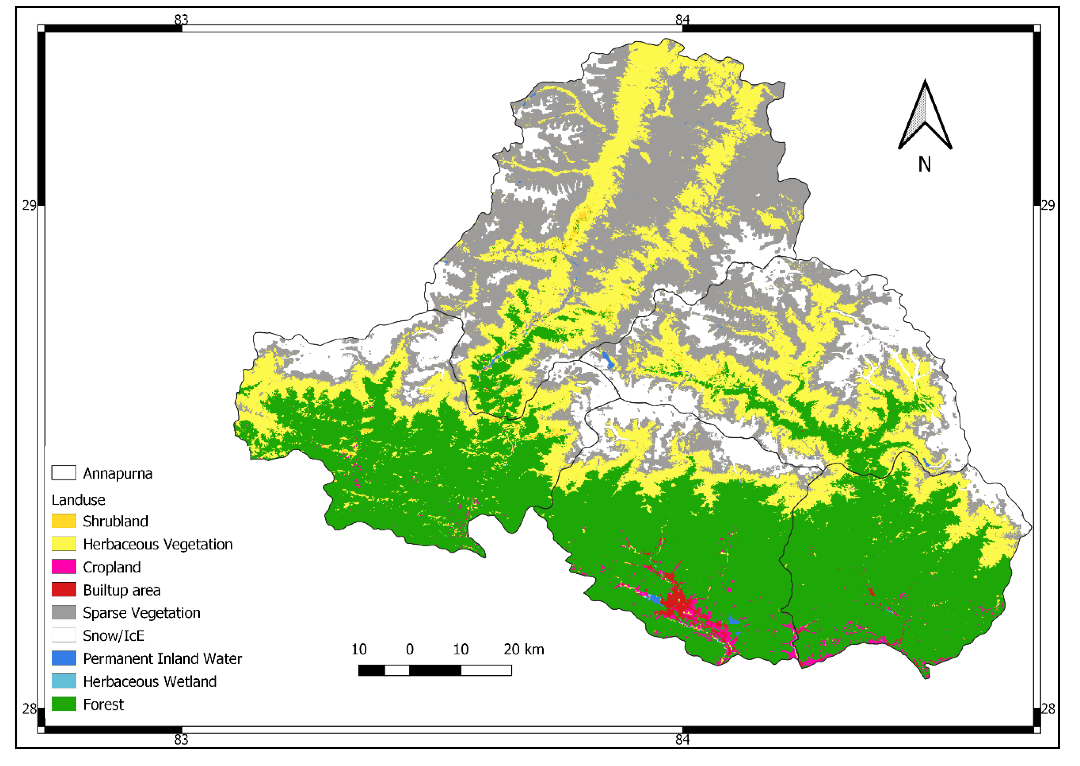
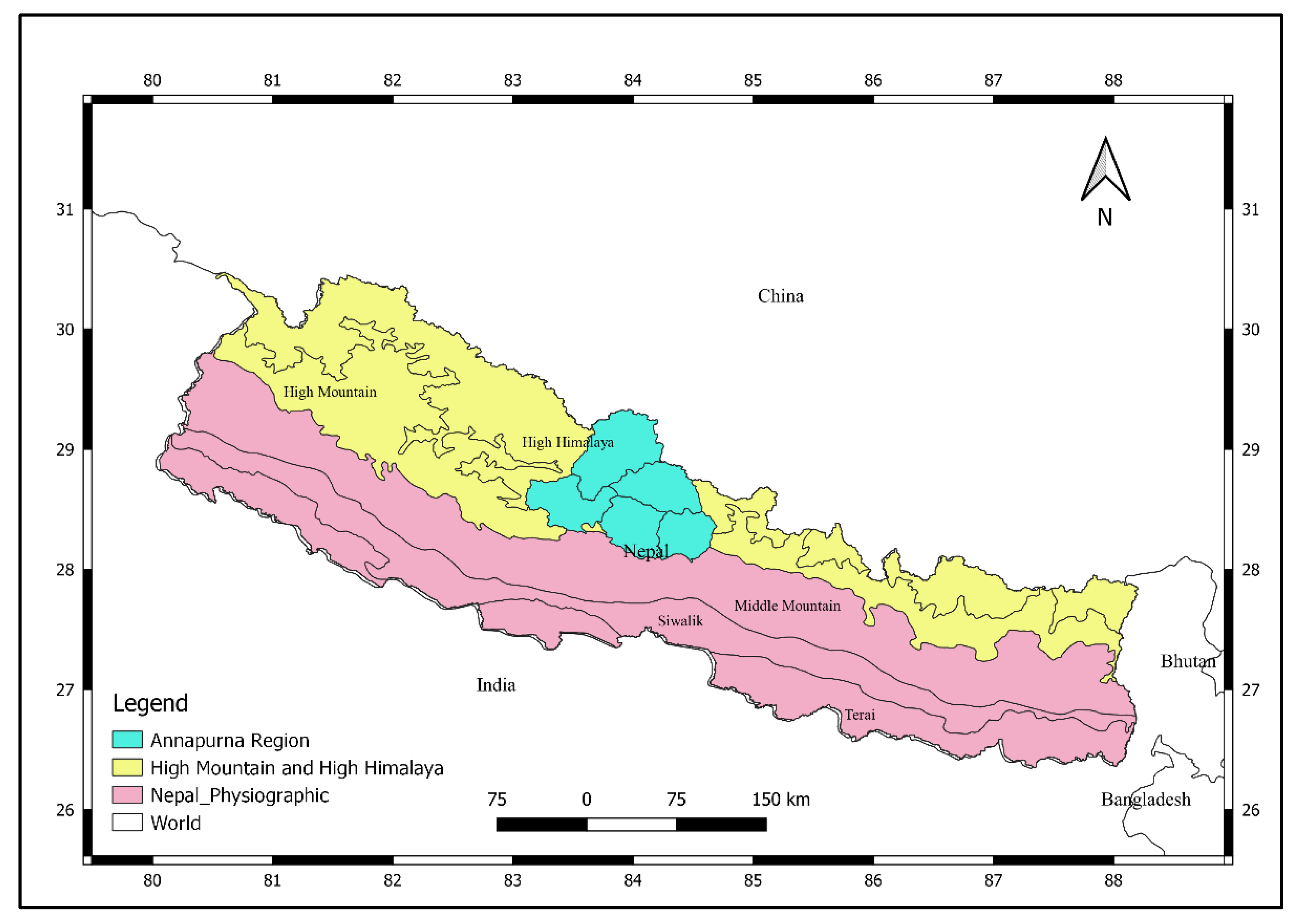
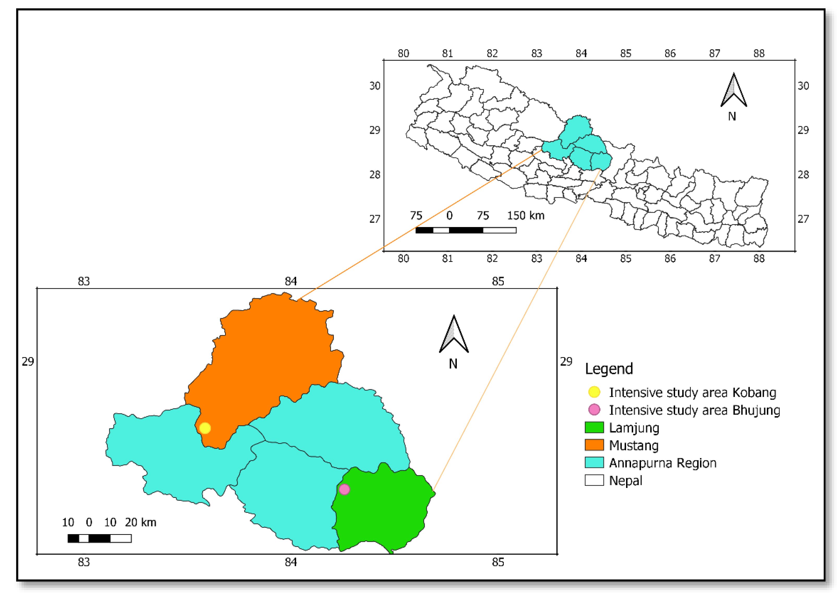
2.1. Study Area
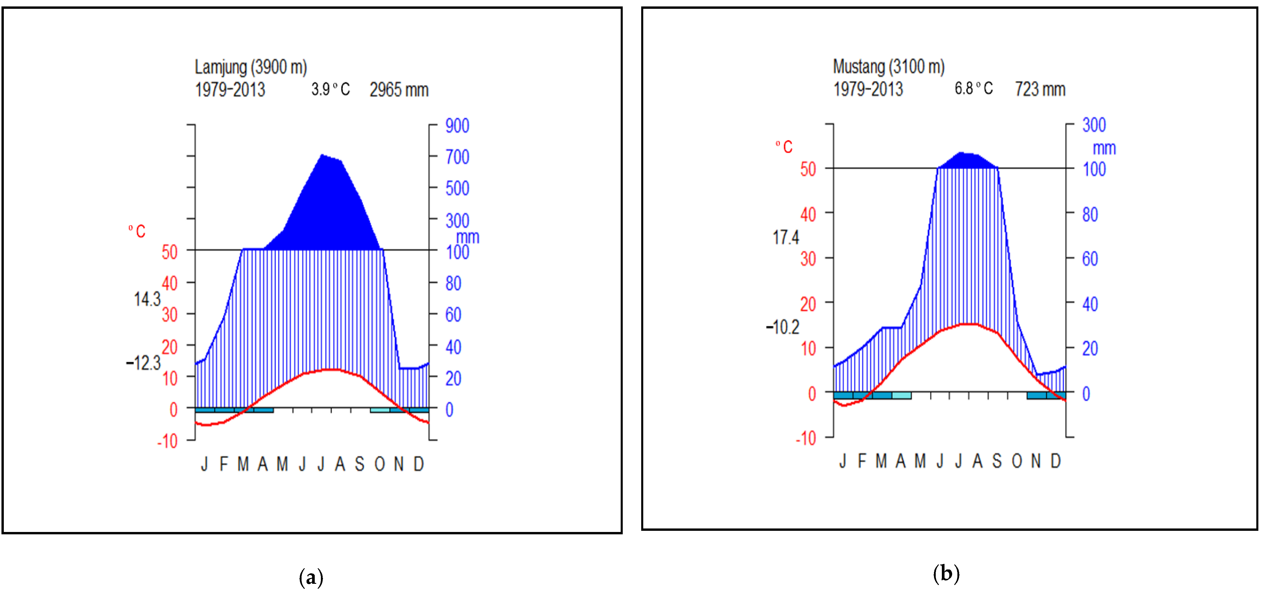
2.2. Climatic Conditions in the Intensive Study Sites
2.3. Geology and Soil in the Intensive Study Area
2.4. Data Collection
2.5. Data Analysis
3. Results
3.1. Forest Composition
3.1.1. Species Recorded and Their Main Features
3.1.2. Species Evenness, Richness, and Diversity
3.1.3. Species Distribution
3.2. Forest Structure
3.2.1. Diameter Frequency Distribution
3.2.2. Main Stand Variables and Health Attributes of Trees
3.2.3. Leaf Sizes of Mountainous Tree Species
4. Discussion
5. Conclusions
Author Contributions
Funding
Institutional Review Board Statement
Informed Consent Statement
Data Availability Statement
Acknowledgments
Conflicts of Interest
Appendix A

| Land Cover | Area (km2) | Percentage |
|---|---|---|
| Forest | 4300.70 | 36.05 |
| Sparse vegetation | 3095.07 | 25.94 |
| Herbaceous vegetation | 2781.35 | 23.32 |
| Snow/Ice | 1486.45 | 12.46 |
| Cropland | 99.43 | 0.83 |
| Shrubland | 90.45 | 0.76 |
| Built up area | 49.92 | 0.42 |
| Permanent inland water | 18.93 | 0.16 |
| Herbaceous wetland | 7.08 | 0.06 |
| Total | 11,929.37 | 100.00 |
Appendix B
| Test | Method |
|---|---|
| Soil Texture | Hydrometer method [155] |
| pH | 1:2 soil water suspension [156] |
| Organic matter content (OM, %) | Walkely and Black [157] |
| Total Nitrogen content (N, %) | Kjeldahl method [158] |
| Available Phosphorus (P205, kg ha−1) | Olsen′s bicarbonate [159] |
| Available Potassium (K20, kg ha−1) | Flame photometry [160] |
| Properties | Rating |
|---|---|
| pH | IF > 7.5, “Alkaline”, IF > 6.4, “Neutral”, “Acidic” |
| O.M. | IF > 5, “High”, IF > 2.4, “Medium”, “Low” |
| N. | IF > 0.2, “High”, IF > 0.1, “Medium”, “Low” |
| P2O5 | IF > 55, “High”, IF > 31, “Medium”, “Low” |
| K2O | IF > 280, “High”, IF> 110, “Medium”, “Low” |
References
- Gairola, S.; Rawal, R.S.; Todaria, N.P. Forest vegetation patterns along an altitudinal gradient in sub-alpine zone of west Himalaya, India. Afr. J. Plant Sci. 2008, 2, 042–048. [Google Scholar]
- Timilsina, N.; Ross, M.S.; Heinen, J.T. A community analysis of sal (Shorea robusta) forests in the western Terai of Nepal. For. Ecol. Manag. 2007, 241, 223–234. [Google Scholar] [CrossRef]
- Ahmad, I.; Ahmad, M.S.A.; Hussain, M.; Ashraf, M.; Ashraf, M.Y. Spatio-temporal variations in soil characteristics and nutrient availability of an open scrub type rangeland in the sub-mountainous Himalayan tract of Pakistan. Pak. J. Bot. 2011, 43, 565–571. [Google Scholar]
- Gutiérrez, A.G.; Huth, A. Successional stages of primary temperate rainforests of Chiloé Island, Chile. Pers. Plant. Ecol. Evol. Syst. 2012, 14, 243–256. [Google Scholar] [CrossRef]
- Canadell, J.G.; Le Quéré, C.; Raupach, M.R.; Field, C.B.; Buitenhuis, E.T.; Ciais, P.; Conway, T.J.; Gillett, N.P.; Houghton, R.A.; Marland, G. Contributions to accelerating atmospheric CO2 growth from economic activity, carbon intensity, and efficiency of natural sinks. Proc. Natl. Acad. Sci. USA 2007, 104, 18866–18870. [Google Scholar] [CrossRef] [Green Version]
- Khaine, I.; Woo, S.Y. An overview of interrelationship between climate change and forests. For. Sci. Technol. 2014, 11, 11–18. [Google Scholar] [CrossRef]
- Sullivan, M.J.P.; Talbot, J.; Lewis, S.L.; Phillips, O.L.; Qie, L.; Begne, S.K.; Chave, J.; Cuni-Sanchez, A.; Hubau, W.; Lopez-Gonzalez, G.; et al. Diversity and carbon storage across the tropical forest biome. Sci. Rep. 2017, 7, 39102. [Google Scholar] [CrossRef] [Green Version]
- Grubb, P.J. Control of forest growth and distribution on wet tropical mountains: With special reference to mineral nutrition. Annu. Rev. Ecol. Syst. 1977, 8, 83–107. [Google Scholar] [CrossRef]
- Lieberman, D.; Lieberman, M.; Peralta, R.; Hartshorn, G.S. Tropical forest structure and composition on a large-scale altitudinal gradient in Costa Rica. J. Ecol. 1996, 84, 137–152. [Google Scholar] [CrossRef]
- Koch, G.W.; Sillett, S.C.; Jennings, G.M.; Davis, S.D. The limits to tree height. Nature 2004, 428, 851–854. [Google Scholar] [CrossRef]
- Chave, J.; Réjou-Méchain, M.; Búrquez, A.; Chidumayo, E.; Colgan, M.S.; Delitti, W.B.; Duque, A.; Eid, T.; Fearnside, P.M.; Goodman, R.C.; et al. Improved allometric models to estimate the aboveground biomass of tropical trees. Glob. Change Biol. 2014, 20, 3177–3190. [Google Scholar] [CrossRef] [PubMed]
- Toledo, M.; Poorter, L.; Peña-Claros, M.; Alarcón, A.; Balcázar, J.; Leaño, C.; Lianque, O.; Vroomans, V.; Zuidema, P.; Bongers, F. Climate is a stronger driver of tree and forest growth rates than soil and disturbance. J. Ecol. 2011, 99, 254–264. [Google Scholar] [CrossRef]
- Walther, G.R. Community and ecosystem responses to recent climate change. Phil. Trans. Ro. Soc. B Biol. Sci. 2010, 365, 2019–2024. [Google Scholar] [CrossRef]
- Beckage, B.; Osborne, B.; Gavin, D.G.; Pucko, C.; Siccama, T.; Perkins, T. A rapid upward shift of a forest ecotone during 40 years of warming in the Green Mountains of Vermont. Proc. Natl. Acad. Sci. USA 2008, 105, 4197–4202. [Google Scholar] [CrossRef] [PubMed] [Green Version]
- Kullman, L.; Öberg, L. Post-Little Ice Age tree line rise and climate warming in the Swedish Scandes: A landscape ecological perspective. J. Ecol. 2009, 97, 415–429. [Google Scholar] [CrossRef]
- Field, R.; ÓBrien, E.M.; Whittaker, R.J. Global models for predicting woody plant richness from climate: Development and evaluation. Ecology 2005, 86, 2263–2277. [Google Scholar] [CrossRef] [Green Version]
- Francis, A.P.; Currie, D.J. A globally consistent richness-climate relationship for angiosperms. Am. Nat. 2003, 161, 523–536. [Google Scholar] [CrossRef]
- Gillman, L.N.; Wright, S.D. Species richness and evolutionary speed: The influence of temperature, water and area. J. Biogeogr. 2014, 41, 39–51. [Google Scholar] [CrossRef]
- Goldie, X.; Gillman, L.; Crisp, M.; Wright, S. Evolutionary speed limited by water in arid Australia. Phil. Trans. Ro. Soc. B Biol. Sci. 2010, 277, 2645–2653. [Google Scholar] [CrossRef] [PubMed] [Green Version]
- ÓBrien, E. Water-energy dynamics, climate, and prediction of woody plant species richness: An interim general model. J. Biogeogr. 1998, 25, 379–398. [Google Scholar] [CrossRef]
- Gentry, A.H. Changes in plant community diversity and floristic composition on environmental and geographical gradients. Ann. Mo. Bot. Gard. 1988, 75, 1–34. [Google Scholar] [CrossRef]
- Shrestha, K.B.; Hofgaard, A.; Vandvik, V. Recent tree line dynamics are similar between dry and mesic areas of Nepal, central Himalaya. J. Plant. Ecol. 2015, 8, 347–358. [Google Scholar] [CrossRef] [Green Version]
- Ter Steege, H.; Pitman, N.C.; Phillips, O.L.; Chave, J.; Sabatier, D.; Duque, A.; Molino, J.F.; Prévost, M.F.; Spichiger, R.; Castellanos, H.; et al. Continental-scale patterns of canopy tree composition and function across Amazonia. Nature 2006, 443, 444–447. [Google Scholar] [CrossRef] [PubMed]
- Hall, J.B.; Swaine, M. Classification and ecology of closed-canopy forest in Ghana. J. Ecol. 1976, 64, 913–951. [Google Scholar] [CrossRef]
- Bongers, F.; Poorter, L.; Van Rompaey, R.S.A.R.; Parren, M. Distribution of twelve moist forest canopy tree species in Liberia and Cote d’Ivoire: Response curves to a climatic gradient. J. Vegt. Sci. 1999, 10, 371–382. [Google Scholar] [CrossRef]
- Engelbrecht, B.M.; Comita, L.S.; Condit, R.; Kursar, T.A.; Tyree, M.T.; Turner, B.L.; Hubbell, S.P. Drought sensitivity shapes species distribution patterns in tropical forests. Nature 2007, 447, 80–82. [Google Scholar] [CrossRef]
- Swaine, M.D. Precipitation and soil fertility as factors limiting forest species distributions in Ghana. J. Ecol. 1996, 84, 419–428. [Google Scholar] [CrossRef]
- Toledo, M.; Peña-Claros, M.; Bongers, F.; Alarcón, A.; Balcázar, J.; Chuviña, J.; Claudio, L.; Licona, J.C.; Poorter, L. Distribution patterns of tropical woody species in response to climatic and edaphic gradients. J. Ecol. 2012, 100, 253–263. [Google Scholar] [CrossRef]
- Mainali, J.; All, J.; Jha, P.K.; Bhuju, D.R. Responses of montane forest to climate variability in the central Himalayas of Nepal. Mt. Res. Dev. 2015, 35, 66–77. [Google Scholar] [CrossRef]
- Diekmann, M. Species indicator values as an important tool in applied plant ecology—A review. Basic. Appl. Ecol. 2003, 4, 493–506. [Google Scholar] [CrossRef]
- Karpouzoglou, T.; Dewulf, A.; Perez, K.; Gurung, P.; Regmi, S.; Isaeva, A.; Foggin, M.; Bastiaensen, J.; Van Hecken, G.; Zulkafli, Z.; et al. From present to future development pathways in fragile mountain landscapes. Environ. Sci. Pol. 2020, 114, 606–613. [Google Scholar] [CrossRef]
- Bhutia, Y.; Gudasalamani, R.; Ganesan, R.; Saha, S. Assessing forest structure and composition along the altitudinal gradient in the state of Sikkim, Eastern Himalayas, India. Forests 2019, 10, 633. [Google Scholar] [CrossRef] [Green Version]
- Kalacska, M.; Sanchez-Azofeifa, G.A.; Calvo-Alvarado, J.C.; Quesada, M.; Rivard, B.; Janzen, D.H. Species composition, similarity and diversity in three successional stages of a seasonally dry tropical forest. For. Ecol. Manag. 2004, 200, 227–247. [Google Scholar] [CrossRef]
- Feroz, S.M.; Kabir, M.E.; Hagihara, A. Species composition, diversity, and stratification in subtropical evergreen broadleaf forests along a latitudinal thermal gradient in the Ryukyu Archipelago, Japan. Glob. Ecol. Conserv. 2015, 4, 63–72. [Google Scholar] [CrossRef] [Green Version]
- Johnson, C.; Chhin, S.; Zhang, J. Effects of climate on competitive dynamics in mixed conifer forests of the Sierra Nevada. For. Ecol. Manag. 2017, 394, 1–12. [Google Scholar] [CrossRef]
- Nlungu-Kweta, P.; Leduc, A.; Bergeron, Y. Climate and disturbance regime effects on aspen (Populus tremuloides Michx.) stand structure and composition along an east–west transect in Canada’s boreal forest. Forestry Int. J. For. Res. 2017, 90, 70–81. [Google Scholar]
- Department of Forest Research and Survey (DFRS). High Mountains and High Himal Forests of Nepal; Forest Resource Assessment (FRA) Nepal, Department of Forest Research and Survey: Kathmandu, Nepal, 2015. Available online: https://frtc.gov.np/downloadfile/high%20mountain_1470116949_1579845426.pdf (accessed on 10 October 2020).
- Carter, H.A. Classification of the Himalaya. Am. Alp. J. 1985, 27, 127–129. [Google Scholar]
- European Union, Copernicus Land Monitoring Service (Eu-Copernicus). Copernicus Global Land Service; European Union: Brussels, Belgium, 2020. Available online: https://land.copernicus.eu/global/products (accessed on 10 October 2020).
- Annapurna Conservation Area (ACA). Management plan of Annapurna Conservation Area. Nepal Trust for Nature Conservation, 2009–2012; Nepal Trust for Nature Conservation: Kathmandu, Nepal, 2009.
- Dhar, O.N.; Nandargi, S. Areas of heavy precipitation in the Nepalese Himalayas. Weather 2005, 60, 354–356. [Google Scholar] [CrossRef]
- Biodiversity Profiles Project (BPP). Biodiversity Assessment of Forest Ecosystems of the Western Mid-Hills of Nepal; Biodiversity Profiles Project, Publication No. 7; Department of National Parks and Wildlife Conservation: Kathmandu, Nepal, 1995.
- Biodiversity Profiles Project (BPP). Biodiversity Assessment of Forest Ecosystems of the Central Mid-Hills of Nepal; Biodiversity Profiles Project, Publication No. 8; Department of National Parks and Wildlife Conservation: Kathmandu, Nepal, 1995.
- Department of National Parks and Wildlife Conservation (DNPWC). Protected Areas of Nepal; Ministry of Forests and Environment. Department of National Parks and Wildlife Conservation: Kathmandu, Nepal, 2018. Available online: http://www.dnpwc.gov.np/media/publication/Protected_Area_of_Nepal-2075.pdf (accessed on 12 September 2020).
- Karger, D.N.; Conrad, O.; Böhner, J.; Kawohl, T.; Kreft, H.; Soria-Auza, R.W.; Zimmermann, N.E.; Linder, H.P.; Kessler, M. Climatologies at high resolution for the Earth’s land surface areas. Sci. Dat. 2017, 4, 170122. [Google Scholar] [CrossRef] [Green Version]
- Bohner, J. General climatic controls and topo climatic variations in Central and High Asia. Boreas 2006, 35, 279–295. [Google Scholar] [CrossRef]
- Government of Nepal, Ministry of Forests and Soil Conservation (GoN/MoFSC). Nepal National Biodiversity Strategy and Action Plan 2014–2020; Government of Nepal, Ministry of Forests and Soil Conservation: Kathmandu, Nepal, 2014. Available online: https://www.cbd.int/doc/world/np/np-nbsap-v2-en.pdf (accessed on 16 September 2020).
- Karki, R.; Hasson, S.; Schickhoff, U.; Scholten, T.; Böhner, J. Rising Precipitation Extremes across Nepal. Climate 2017, 5, 4. [Google Scholar] [CrossRef] [Green Version]
- Karki, R.; Talchabhadel, R.; Aalto, J.; Baidya, S.K. New climatic classification of Nepal. Theor. Appl. Climatol. 2016, 125, 799–808. [Google Scholar] [CrossRef]
- Walter, H.; Lieth, H. World Atlas of Climate Diagrams; Part 3; VEB Gustav Fischer Verlag: Jena, Germany, 1967. [Google Scholar]
- Guijarro, J.A. Climatol: Climate Tools (Series Homogenization and Derived Products). 2019. Available online: https://cran.r-project.org/web/packages/climatol/index.html (accessed on 16 September 2020).
- R Studio Team. RStudio: Integrated Development for R; Version 1.3; R Studio: Boston, MA, USA, 2021; Available online: http://www.rstudio.com/ (accessed on 10 January 2021).
- Parsons, A.J.; Law, R.D.; Searle, M.P.; Phillips, R.J.; Lloyd, G.E. Geology of the Dhaulagiri-Annapurna-Manaslu Himalaya, Western Region, Nepal. 1: 200,000. J. Map. 2016, 12, 100–110. [Google Scholar] [CrossRef]
- Hodges, K.V.; Parrish, R.R.; Searle, M.P. Tectonic evolution of the central Annapurna range, Nepalese Himalayas. Tectonics 1996, 15, 1264–1291. [Google Scholar] [CrossRef]
- Dahal, J.; Chidi, C.L.; Mandal, U.K.; Karki, J.; Khanal, N.R.; Pantha, R.H. Physico-chemical properties of soil in Jita and Taksar area of Lamjung district, Nepal. Geo. J. Nepal. 2018, 11, 45–62. [Google Scholar] [CrossRef] [Green Version]
- Pandey, S.; Bhatta, N.P.; Paudel, P.; Pariyar, R.; Maskey, K.H.; Khadka, J.; Thapa, T.B.; Rijal, B.; Panday, D. Improving fertilizer recommendations for Nepalese farmers with the help of soil-testing mobile van. J. Crop. Dev. 2018, 32, 19–32. [Google Scholar] [CrossRef] [Green Version]
- Department of Forests (DoF). Community Forest Inventory Guideline; Department of Forests: Kathmandu, Nepal, 2004.
- Kleinn, C.; Traub, B.; Hoffmann, C. A note on the slope correction and the estimation of the length of line features. Can. J. Forest Res. 2002, 32, 751–756. [Google Scholar] [CrossRef]
- Miehe, G. Vegetationsgeographische Untersuchungen im Dhaulagiri-und Annapurna-Himalaya. Diss. Bot. 1982, 66, 1–2. [Google Scholar]
- Schickhoff, U. The Upper Timberline in the Himalayas, Hindu Kush and Karakorum: A Review of Geographical and Ecological Aspects. In Mountain Ecosystems; Broll, G., Keplin, B., Eds.; Springer: Berlin/Heidelberg, Germany, 2005; pp. 275–354. [Google Scholar]
- Udas, E. The influence of climate variability on growth performance of Abies spectabilis at tree line of West-Central Nepal. Master’s Thesis, University of Greifswald, Greifswald, Germany, 2009. [Google Scholar]
- Beckschäfer, P.; Seidel, D.; Kleinn, C.; Xu, J. On the exposure of hemispherical photographs in forests. iForest-Biogeosci. For. 2013, 6, 228–237. [Google Scholar] [CrossRef] [Green Version]
- Černý, J.; Pokorný, R.; Haninec, P.; Bednář, P. Leaf area index estimation using three distinct methods in pure deciduous stands. J. Vis. Exp. 2019, 150, e59757. [Google Scholar] [CrossRef]
- Getman-Pickering, Z.L.; Campbell, A.; Aflitto, N.; Grele, A.; Davis, J.K.; Ugine, T.A. Leaf Byte: A mobile application that measures leaf area and herbivory quickly and accurately. Meth. Ecol. Evol. 2020, 11, 215–221. [Google Scholar] [CrossRef] [Green Version]
- Razali, N.M.; Wah, Y.B. Power comparisons of Shapiro-Wilk, Kolmogorov-Smirnov, Lilliefors and Anderson-Darling tests. J. Stat. Model. Anal. 2011, 2, 21–33. [Google Scholar]
- Margalef, R. Information theory in ecology. Gen. Syst. Bul. 1958, 3, 36–71. [Google Scholar]
- Pielou, E.C. The measurement of diversity in different types of biological collections. J. Theor. Biol. 1966, 13, 131–144. [Google Scholar] [CrossRef]
- Oksanen, J.; Guillaume Blanchet, F.; Friendly, M.; Kindt, R.; Legendre, P.; McGlinn, D.; Minchin, P.R.; ÓHara, R.B.; Simpson, G.L.; Solymos, P.; et al. Vegan: Community Ecology Package. 2019. Available online: https://cran.r-project.org/web/packages/vegan/index.html (accessed on 10 September 2020).
- Shannon, C.E.; Wiener, W. The Mathematical Theory of Communication, 1st ed; Urban University Illinois Press: Champaign, IL, USA, 1963; 125p. [Google Scholar]
- Simpson, E.H. Measurement of diversity. Nature 1949, 163, 688. [Google Scholar] [CrossRef]
- Gadow, K.V.; Zhang, C.Y.; Wehenkel, C.; Pommerening, A.; Corral-Rivas, J.; Korol, M.; Myklush, S.; Hui, G.Y.; Kiviste, A.; Zhao, X.H. Forest structure and diversity. In Continuous Cover Forestry; Pukkala, T., von Gadow, K., Eds.; Springer: Dordrecht, The Netherlands, 2012; pp. 29–83. [Google Scholar]
- Lima, R.B.; Bufalino, L.; Alves Junior, F.T.; Silva, J.A.D.; Ferreira, R.L. Diameter distribution in a Brazilian tropical dry forest domain: Predictions for the stand and species. Anais da Academia Brasileira de Ciências 2017, 89, 1189–1203. [Google Scholar] [CrossRef] [Green Version]
- Wickham, H. Tidyverse: Easily Install and Load the ‘Tidyversé. 2019. Available online: https://cran.r-project.org/web/packages/tidyverse/index.html (accessed on 11 September 2020).
- Wickham, H.; Chang, W.; Henry, L.; Pedersen, T.L. ggplot2: Create Elegant Data Visualizations Using the Grammar of Graphics. 2019. Available online: https://cran.r-project.org/web/packages/ggplot2/index.html (accessed on 20 September 2020).
- Curtis, J.T.; Mcintosh, R.P. The interrelations of certain analytic and synthetic phytosociological characters. Ecology 1950, 31, 434–455. [Google Scholar] [CrossRef]
- Schindelin, J.; Arganda-Carreras, I.; Frise, E.; Kaynig, V.; Longair, M.; Pietzsch, T.; Preibisch, S.; Rueden, C.; Saalfeld, S.; Schmid, B.; et al. Fiji: An open-source platform for biological-image analysis. Nat. Meth. 2012, 9, 676–682. [Google Scholar] [CrossRef] [Green Version]
- Beckschäfer, P. Hemispherical_2. 0–Batch Processing Hemispherical and Canopy Photographs with ImageJ–User Manual; University of Göttingen: Göttingen, Germany, 2015; Available online: https://docplayer.net/55833385-Hemispherical_2-0-batch-processing-hemispherical-and-canopy-photographs-with-imagej-user-manual-by-philip-beckschafer-january-2015.html (accessed on 12 August 2020).
- Wilcoxon, F. Individual comparisons by ranking methods. Biom. Bull. 1945, 1, 80–83. [Google Scholar] [CrossRef]
- Zobel, D.B.; Singh, S.P. Himalayan forests and ecological generalizations. Bioscience 1997, 47, 735. [Google Scholar] [CrossRef]
- Tree Improvement and Silviculture Component (TISC). Forest and Vegetation Types of Nepal; Natural Resource Management Sector Assistance Program Nepal, Tree Improvement and Silviculture Component; Document Series 105; Tree Improvement and Silviculture Component: Kathmandu, Nepal, 2002. [Google Scholar]
- Miehe, G.; Pendry, C.; Chaudhary, R.P. Nepal: An Introduction to the Natural History, Ecology and Human Environment of the Himalayas: A Companion Volume to the Flora of Nepal; Royal Botanic Garden Edinburgh: Edinburgh, Scotland, 2015. [Google Scholar]
- Rajbhandari, K.R.; Watson, M. Rhododendrons of Nepal (Fascicle of Flora of Nepal); Department of Plant Resources: Kathmandu, Nepal, 2005; Volume 5.
- Pradhan, S.; Saha, G.K.; Khan, J.A. Ecology of the red panda Ailurus fulgens in the Singhalila National Park, Darjeeling, India. Biol. Conserv. 2001, 98, 11–18. [Google Scholar] [CrossRef]
- Tiwari, A.; Jha, P.K. An overview of tree line response to environmental changes in Nepal Himalaya. Trop. Ecol. 2018, 59, 273–285. [Google Scholar]
- Chhetri, P.K. Dendrochronological Analyses and Climate Change Perceptions in Langtang National Park, Central Nepal. In Climate Change and Disaster Impact Reduction; Aryal, K.R., Gadema, Z., Eds.; Northumbria University: Newcastle, UK, 2008. [Google Scholar]
- District Development Committee (DDC). Resource Mapping Report of Mustang District; District Development Committee: Jomsom, Mustang, 2014.
- Christensen, M.; Heilmann-Clausen, J. Forest biodiversity gradients and the human impact in Annapurna Conservation Area, Nepal. Biodvers. Conserv. 2009, 18, 2205–2221. [Google Scholar] [CrossRef]
- Jnawali, S.R.; Baral, H.S.; Lee, S.; Acharya, K.P.; Upadhyay, G.P.; Pandey, M.; Shrestha, R.; Joshi, D.; Lamichhane, B.R.; Griffiths, J.; et al. The Status of Nepal’s Mammals: The National Red List Series-IUCN; IUCN-SSC and National Trust of Nature Conservation: Kathmandu, Nepal, 2011. [Google Scholar]
- Bista, D.; Shrestha, S.; Sherpa, P.; Thapa, G.J.; Kokh, M.; Lama, S.T.; Khanal, K.P.; Thapa, A.; Jnawali, S.R. Distribution and habitat use of red panda in the Chitwan-Annapurna Landscape of Nepal. PLoS ONE 2017, 12, e0178797. [Google Scholar] [CrossRef] [PubMed] [Green Version]
- Bhattarai, S.; Chaudhary, R.P.; Taylor, R.S. The use of plants for fencing and fuelwood in Mustang District, Trans-Himalayas, Nepal. Sci. World 2009, 7, 59–63. [Google Scholar] [CrossRef]
- Chapagain, N.R.; Chetri, M. Biodiversity Profile of Upper Mustang; National Trust for Nature Conservation, Annapurna Conservation Area Project, Upper Mustang Biodiversity Conservation Project: Kathmandu, Nepal, 2006. [Google Scholar]
- Dobremez, J.F. Nepal: Ecology and Biogeography; Éditions du Centre National de la Recherche Scientifique: Paris, France, 1976. [Google Scholar]
- Stainton, J.D.A. Forest of Nepal; John Murrey: London, UK, 1972. [Google Scholar]
- Bhuju, S.; Gauchan, D.P. Taxus wallichiana (Zucc.), an Endangered Anti-Cancerous Plant: A Review. Int. J. Res. 2018, 5, 10–21. [Google Scholar]
- Leilei, L.; Jianrong, F.; Yang, C. The relationship analysis of vegetation cover, precipitation and land surface temperature based on remote sensing in Tibet, China. In Proceedings of the IOP Conference Series: Earth and Environmental Science (Vol. 17, No. 1, p. 012034), International Symposium on Remote Sensing of Environment (ISRSE35), Beijing, China, 22–26 April 2013. [Google Scholar]
- Joshi, N.; Gyawali, P.; Sapkota, S.; Neupane, D.; Shrestha, S.; Shrestha, N.; Tuladhar, F.M. Analyzing the effect of climate change (precipitation and temperature) on vegetation cover of Nepal using time-series MODIS images. Ann. Photogram. Remote Sens. Spatial Inf. Sci. 2019, 209–216. [Google Scholar]
- Daniels, L.D.; Veblen, T.T. Spatiotemporal influences of climate on altitudinal tree line in northern Patagonia. Ecology 2004, 85, 1284–1296. [Google Scholar] [CrossRef] [Green Version]
- Elliott, G.P.; Kipfmueller, K.F. Multi-scale influences of climate on upper tree line dynamics in the southern Rocky Mountains, USA: Evidence of intraregional variability and bioclimatic thresholds in response to twentieth century warming. Ann. Assoc. Am. Geogr. 2011, 101, 1181–1203. [Google Scholar] [CrossRef]
- Danby, R.K.; Hik, D.S. Variability, contingency, and rapid change in recent subarctic alpine tree line dynamics. J. Ecol. 2007, 95, 352–363. [Google Scholar] [CrossRef]
- Elliott, G.P.; Kipfmueller, K.F. Multi-scale influences of slope aspect and spatial pattern on ecotonal dynamics at upper tree line in the southern Rocky Mountains, USA. Arct. Antarct. Alp. Res. 2010, 42, 45–56. [Google Scholar] [CrossRef] [Green Version]
- Paudel, P.K.; Bhattarai, B.P.; Kindlmann, P. An overview of the biodiversity in Nepal. In Himalayan Biodiversity in the Changing World; Kindalmann, P., Ed.; Springer: Dordrecht, The Netherlands, 2012; pp. 1–40. [Google Scholar]
- Bhuju, D.R.; Gaire, N.P. Tree-Rings and Tree Lines of Nepal Himalaya; Research Synopsis, Commemorating Symposium Himalayan Tree-Line; Tree-Ring Society of Nepal: Katmandu, Nepal, 2017. [Google Scholar]
- Singh, J.S.; Singh, S.P. Forest vegetation of the Himalaya. The Bot. Rev. 1987, 53, 80–192. [Google Scholar] [CrossRef]
- Vetaas, O.R.; Grytnes, J.A. Distribution of vascular plant species richness and endemic richness along the Himalayan elevation gradient in Nepal. Glob. Ecol. Biogeogr. 2002, 11, 291–301. [Google Scholar] [CrossRef]
- Paudel, S.; Vetaas, O.R. Effects of topography and land use on woody plant species composition and beta diversity in an arid Trans-Himalayan landscape, Nepal. J. Mt. Sci. 2014, 11, 1112–1122. [Google Scholar] [CrossRef]
- Kharal, D.K.; Meilby, H.; Rayamajhi, S.; Bhuju, D.; Thapa, U.K. Tree ring variability and climate response of Abies spectabilis along an elevation gradient in Mustang, Nepal. Banko Janakari 2014, 24, 3–13. [Google Scholar] [CrossRef] [Green Version]
- Kharkwal, G.; Mehrotra, P.; Rawat, Y.S.; Pangtey, Y.P.S. Phytodiversity and growth form in relation to altitudinal gradient in the Central Himalayan (Kumaun) region of India. Curr. Sci. 2005, 873–878. [Google Scholar]
- Manish, K.; Telwala, Y.; Nautiyal, D.C.; Pandit, M.K. Modelling the impacts of future climate change on plant communities in the Himalaya: A case study from Eastern Himalaya, India. Model. Earth Syst. Environ. 2016, 2, 92. [Google Scholar] [CrossRef] [Green Version]
- Sharma, N.; Behera, M.D.; Das, A.P.; Panda, R.M. Plant richness pattern in an elevation gradient in the Eastern Himalaya. Biodivers. Conserv. 2019, 28, 2085–2104. [Google Scholar] [CrossRef]
- Ghimire, B.; Mainali, K.P.; Lekhak, H.D.; Chaudhary, R.P.; Ghimeray, A.K. Regeneration of Pinus wallichiana AB Jackson in a trans-Himalayan dry valley of north-central Nepal. Himal. J. Sci. 2010, 6, 19–26. [Google Scholar]
- Måren, I.E.; Karki, S.; Prajapati, C.; Yadav, R.K.; Shrestha, B.B. Facing north or south: Does slope aspect impact forest stand characteristics and soil properties in a semiarid trans-Himalayan valley? J. Arid. Environ. 2015, 121, 112–123. [Google Scholar] [CrossRef] [Green Version]
- Olivero, A.M.; Hix, D.M. Influence of aspect and stand age on ground flora of Southeastern Ohio forest ecosystems. Plant Ecol. 1998, 139, 177–187. [Google Scholar] [CrossRef]
- Schickhoff, U. Contributions to the synecology and syntaxonomy of West Himalayan coniferous forest communities. Phytoeco. 1996, 26, 537–581. [Google Scholar] [CrossRef]
- Zavaleta, E.S.; Shaw, M.R.; Chiariello, N.R.; Thomas, B.D.; Cleland, E.E.; Field, C.B.; Mooney, H.A. Grassland responses to three years of elevated temperature, CO2, precipitation, and N deposition. Ecol. Monogr. 2003, 73, 585–604. [Google Scholar] [CrossRef] [Green Version]
- Stevens, M.H.H.; Shirk, R.; Steiner, C.E. Water and fertilizer have opposite effects on plant species richness in a mesic early successional habitat. Plant. Ecol. 2006, 183, 27–34. [Google Scholar] [CrossRef]
- Yang, H.; Li, Y.; Wu, M.; Zhang, Z.H.E.; Li, L.; Wan, S. Plant community responses to nitrogen addition and increased precipitation: The importance of water availability and species traits. Glob. Change. Biol. 2011, 17, 2936–2944. [Google Scholar] [CrossRef]
- Yoda, K. A preliminary survey of forest vegetation of eastern Nepal. J. Coll. Art. Sci. 1967, 5, 99–140. [Google Scholar]
- Stevens, G.C. The elevational gradient in altitudinal range: An extension of Rapoport’s latitudinal rule to altitude. Am. Nat. 1992, 140, 893–911. [Google Scholar] [CrossRef]
- Bhattarai, K.R.; Vetaas, O.R. Can Rapoport’s rule explain tree species richness along the Himalayan elevation gradient, Nepal? Divers. Distb. 2006, 12, 373–378. [Google Scholar] [CrossRef]
- Kluge, J.; Worm, S.; Lange, S.; Long, D.; Böhner, J.; Yangzom, R.; Miehe, G. Elevational seed plants richness patterns in Bhutan, Eastern Himalaya. J. Biogeogr. 2017, 44, 1711–1722. [Google Scholar] [CrossRef]
- Stan, K.; Sanchez-Azofeifa, A. Tropical dry forest diversity, climatic response, and resilience in a changing climate. Forests 2019, 10, 443. [Google Scholar] [CrossRef] [Green Version]
- Kushwaha, S.P.S.; Nandy, S. Species diversity and community structure in sal (Shorea robusta) forests of two different precipitation regimes in West Bengal, India. Biodivers. Conserv. 2012, 21, 1215–1228. [Google Scholar] [CrossRef]
- Khaine, I.; Woo, S.Y.; Kang, H.; Kwak, M.; Je, S.M.; You, H.; Lee, T.; Jang, J.; Lee, H.K.; Lee, E.; et al. Species diversity, stand structure, and species distribution across a precipitation gradient in tropical forests in Myanmar. Forests 2017, 8, 282. [Google Scholar] [CrossRef] [Green Version]
- Osland, M.J.; Feher, L.C.; Griffith, K.T.; Cavanaugh, K.C.; Enwright, N.M.; Day, R.H.; Stagg, C.L.; Krauss, K.W.; Howard, R.J.; Grace, J.B.; et al. Climatic controls on the global distribution, abundance, and species richness of mangrove forests. Ecol. Monogr. 2017, 87, 341–359. [Google Scholar] [CrossRef] [Green Version]
- Staver, A.C.; Archibald, S.; Levin, S. Tree cover in sub-Saharan Africa: Rainfall and fire constrain forest and savanna as alternative stable states. Ecology 2011, 92, 1063–1072. [Google Scholar] [CrossRef]
- Sharma, C.M.; Ghildiyal, S.K.; Gairola, S.; Suyal, S. Vegetation structure, composition, and diversity in relation to the soil characteristics of temperate mixed broad-leaved forest along an altitudinal gradient in Garhwal Himalaya. Indian J. Sci. Technol. 2009, 2, 39–45. [Google Scholar] [CrossRef]
- Pandey, K.P.; Adhikari, Y.P.; Weber, M. Structure, composition and diversity of forest along the altitudinal gradient in the Himalayas, Nepal. Appl. Ecol. Environ. Res. 2016, 14, 235–251. [Google Scholar] [CrossRef]
- Bhat, J.A.; Kumar, M.; Negi, A.K.; Todaria, N.P.; Malik, Z.A.; Pala, N.A.; Kumar, A.; Shukla, G. Altitudinal gradient of species diversity and community of woody vegetation in the Western Himalayas. Glob. Eco. Cons. 2020, 24, e01302. [Google Scholar]
- Maçaneiro, J.P.D.; Oliveira, L.Z.; Seubert, R.C.; Eisenlohr, P.V.; Schorn, L.A. More than environmental control at local scales: Do spatial processes play an important role in floristic variation in subtropical forests? Acta Bot. Bras. 2016, 30, 183–192. [Google Scholar] [CrossRef] [Green Version]
- Sevegnani, L.; Uhlmann, A.; de Gasper, A.L.; Meyer, L.; Vibrans, A.C. Climate affects the structure of mixed rain forest in southern sector of Atlantic domain in Brazil. Acta Oecol. 2016, 77, 109–117. [Google Scholar] [CrossRef]
- Muñoz Mazón, M.; Klanderud, K.; Finegan, B.; Veintimilla, D.; Bermeo, D.; Murrieta, E.; Delgado, D.; Sheil, D. How forest structure varies with elevation in old growth and secondary forest in Costa Rica. For. Ecol. Manag. 2020, 469, 118191. [Google Scholar] [CrossRef]
- Komárková, V.; Webber, P.J. An Alpine Vegetation Map of Niwot Ridge, Colorado. Arct. Alp. Res. 1978, 10, 1–29. [Google Scholar] [CrossRef]
- Chaurasia, O.P.; Brahma, S. Cold Desert Plants; Volume III-Changthang Valley; Field Research Laboratory, DRDO: Leh, Jammu; Kashmir, India, 1997; Volume 3, p. 85. [Google Scholar]
- Terra, M.D.C.N.S.; Santos, R.M.D.; Prado Júnior, J.A.D.; de Mello, J.M.; Scolforo, J.R.S.; Fontes, M.A.L.; Schiavini, I.; dos Reis, A.A.; Bueno, I.T.; Magnago, L.F.S.; et al. Water availability drives gradients of tree diversity, structure, and functional traits in the Atlantic–Cerrado–Caatinga transition, Brazil. J. Plant. Ecol. 2018, 11, 803–814. [Google Scholar] [CrossRef] [Green Version]
- Sinha, S.; Badola, H.K.; Chhetri, B.; Gaira, K.S.; Lepcha, J.; Dhyani, P.P. Effect of altitude and climate in shaping the forest compositions of Singalila National Park in Khangchendzonga Landscape, Eastern Himalaya, India. J. Asia-Pac. Biodivers. 2018, 11, 267–275. [Google Scholar] [CrossRef]
- Hiltner, U.; Bräuning, A.; Gebrekirstos, A.; Huth, A.; Fischer, R. Impacts of precipitation variability on the dynamics of a dry tropical montane forest. Ecol. Model. 2016, 320, 92–101. [Google Scholar] [CrossRef]
- Beard, J.S. Historical and ecological development of evergreen broadleaved forest of Australia. Vegt. Sci. For. 1995, 12a, 179–187. [Google Scholar]
- Duchesne, L.; Ouimet, R. Relationships between structure, composition, and dynamics of the pristine northern boreal forest and air temperature, precipitation, and soil texture in Quebec (Canada). Intl. J. For. Res. 2009, 2009, 398389. [Google Scholar] [CrossRef] [Green Version]
- Shrestha, B.B.; Ghimire, B.; Lekhak, H.D.; Jha, P.K. Regeneration of tree line birch (Betula utilis D. Don) forest in a trans-Himalayan dry valley in central Nepal. Mt. Res. Dev. 2007, 27, 259–267. [Google Scholar] [CrossRef]
- Dar, J.A.; Sundarapandian, S. Patterns of plant diversity in seven temperate forest types of Western Himalaya, India. J. Asia-Pac. Biodivers. 2016, 9, 280–292. [Google Scholar] [CrossRef] [Green Version]
- Schwab, N. Sensitivity and Response of Alpine Tree Lines to Climate Change-Insights from a Krummholz Tree Line in Rolwaling Himal, Nepal. 2019. Available online: https://ediss.sub.uni-hamburg.de/handle/ediss/8041 (accessed on 24 October 2020).
- Vetaas, O.R. The effect of environmental factors on the regeneration of Quercus semicarpifolia Sm. in central Himalaya, Nepal. Plant. Ecol. 2000, 146, 137–144. [Google Scholar] [CrossRef]
- Uniyal, P.; Pokhriyal, P.; Dasgupta, S.; Bhatt, D.; Todaria, N.P. Plant diversity in two forest types along the disturbance gradient in Dewalgarh Watershed, Garhwal Himalaya. Curr. Sci. 2010, 98, 938–943. [Google Scholar]
- Måren, I.E.; Sharma, L.N. Managing biodiversity: Impacts of legal protection in mountain forests of the Himalayas. Forests 2018, 9, 476. [Google Scholar] [CrossRef] [Green Version]
- Richards, P.W.; Frankham, R.; Walsh, R.P.D. The Tropical Rain Forest: An Ecological Study; Cambridge University Press: Cambridge, UK, 1996. [Google Scholar]
- Francis, W.D. The Development of Buttresses in Queensland Trees; Government Printer: Pretoria, South Africa, 1924.
- Nicoll, B.C.; Ray, D. Adaptive growth of tree root systems in response to wind action and site conditions. Tree Physiol. 1996, 16, 891–898. [Google Scholar] [CrossRef] [PubMed] [Green Version]
- Hernández, L.; Dezzeo, N.; Sanoja, E.; Salazar, L.; Castellanos, H. Changes in structure and composition of evergreen forests on an altitudinal gradient in the Venezuelan Guayana Shield. Revista de Biología Tropical 2012, 60, 11–33. [Google Scholar] [CrossRef] [PubMed] [Green Version]
- Baur, G.N. The Ecological Basis of Rainforest Management; Library AN: 113414, 1965; Food and Agricultural Organization: Rome, Italy, 1965; Available online: http://www.fao.org/3/ax363e/ax363e.pdf (accessed on 1 September 2020).
- Berry, P.E.; Holst, B.K.; Yatskievych, K.; Manara, B. Flora of Venezuelan Guayana. Springer 1998, 53, 1017–1018. [Google Scholar]
- Peppe, D.J.; Royer, D.L.; Cariglino, B.; Oliver, S.Y.; Newman, S.; Leight, E.; Wright, I.J.; Enikolopov, G.; Fernandez-Burgos, M.; Herrera, F.; et al. Sensitivity of leaf size and shape to climate: Global patterns and paleoclimatic applications. New. Phyt. 2011, 190, 724–739. [Google Scholar] [CrossRef] [Green Version]
- McDonald, P.G.; Fonseca, C.R.; Overton, J.M.; Westoby, M. Leaf-size divergence along rainfall and soil-nutrient gradients: Is the method of size reduction common among clades? Funct. Ecol. 2003, 17, 50–57. [Google Scholar] [CrossRef] [Green Version]
- Forest and Agriculture Organization (FAO). Sustainable Forest Management (SFM) Toolbox, Forest Inventory; Forest and Agriculture Organization of United Nations, Rome, Italy. 2021. Available online: http://www.fao.org/sustainable-forest-management/toolbox/modules/forest-inventory/basic-knowledge/en/?type=111 (accessed on 18 June 2021).
- Fischer, C.; Kleinn, C.; Fehrmann, L.; Fuchs, H.; Panferov, O. A national level forest resource assessment for Burkina Faso–A field based forest inventory in a semiarid environment combining small sample size with large observation plots. For. Ecol. Manag. 2011, 262, 1532–1540. [Google Scholar] [CrossRef]
- Bouyoucos, G.J. Directions for making mechanical analyses of soils by the hydrometer method. Soil. Sci. 1936, 42, 225–230. [Google Scholar] [CrossRef]
- Jackson, M.L. Soil chemical analysis, pentice hall of India Pvt. Ltd., New Delhi, India 1973, 498, 151–154. [Google Scholar]
- Walkley, A.; Black, I.A. An examination of the Degtjareff method for determining soil organic matter, and a proposed modification of the chromic acid titration method. Soil. Sci. 1934, 37, 29–38. [Google Scholar] [CrossRef]
- Bremner, J.M.; Mulvaney, C.S. Nitrogen total. In Method of Soil Analysis; Agron. No. 9, Part 2: Chemical and Microbiological Properties, 2nd ed.; Page, A.L., Ed.; American Society of Agronomy: Madison, WI, USA, 1982. [Google Scholar]
- Olsen, S.R. Estimation of Available Phosphorus in Soils by Extraction with Sodium Bicarbonate; US Department of Agriculture: Washington, DC, USA, 1954.
- Toth, S.J.; Prince, A.L. Estimation of cation-exchange capacity and exchangeable Ca, K, and Na contents of soils by flame photometer techniques. Soil. Sci. 1949, 67, 439–446. [Google Scholar] [CrossRef]


| Precipitation Regime | Study Site | Location |
|---|---|---|
| High/Humid | Bhujung, Lamjung (here after “Lamjung”) | 28°22′47″ N, 84°15′27″ E |
| Low/Dry | Kobang, Mustang (here after “Mustang”) | 28°40′29″ N, 83°35′04″ E |
| Study Site | Winter (January–February) (mm) | Pre-Monsoon (March–May) (mm) | Monsoon (June–September) (mm) | Post-Monsoon (October–December) (mm) | Annual (mm) |
|---|---|---|---|---|---|
| Lamjung | 89.41 (64.80) | 441.37 (33.30) | 2273.94 (15.10) | 160.74 (74.19) | 2965.40 (13.00) |
| Mustang | 32.25 (58.10) | 105.08 (31.49) | 535.82 (14.67) | 48.54 (69.29) | 723.00 (12.00) |
| Study Site | Soil Texture | Average Soil pH | Average Soil Organic Matter (%) | Soil Nutrients * | ||
|---|---|---|---|---|---|---|
| Average N (%) | Average P2O5 (Kg ha−1) | Average K2O (Kg ha−1) | ||||
| Lamjung | Loam | 4.75 | 4.70 | 0.23 | 159.73 | 561.00 |
| Mustang | Loam | 6.20 | 5.15 | 0.26 | 154.43 | 561.30 |
| Study Site | Species Name, Recorded Range (Meter above Mean Sea Level) | Number of Trees Inventoried | Main Features |
|---|---|---|---|
| Lamjung | Betula utilis 3700–4000 m | 21 | The only broadleaved species that dominates extensive areas in sub-alpine altitudes [79] and forms tree line vegetation in the Himalayas [80]. |
| Juniperus indica 3900–4000 m | 17 | Found in upper montane woodlands in pure stands or with Abies, Pinus, or in Betula woodland or alpine heath and grassland, these were also reported in the sunny slopes of Mustang [81]. | |
| Rhododendron campanulatum 3700–4000 m | 440 | The major understory component of sub-alpine forest and forms pure stands above the tree line in the Himalayas of Nepal [82]. | |
| Salix nepalensis 3700–4000 m | 26 | Salix spp. colonizes open soil patches after disturbance, and cattle trampling promotes Salix cover. It mainly occurs with alpine dwarf thickets such as Rhododendron [81]. | |
| Sorbus microphylla 3700–4000 m | 45 | This is also called small leaf rowan and its berries are mainly consumed by the red panda (Ailurus fulgens) [83]. It commonly occurs with Betula utilis [81]. | |
| Mustang | Abies spectabilis 3100 m | 65 | The dominant tree in the western and central Himalayas, it grows better in cool and moist north-facing slopes [84]. It occurs as a canopy dominant species along with different species of Rhododendron and Betula utilis [85]. |
| Acer campbellii 3100 m | 65 | The lower Mustang region has mixed forest of Acer, Pinus wallichiana, and Rhododendron spp. [86]. This is one of the less dominant species of the Annapurna region [87]. It forms good habitat for the red panda (Ailurus fulgens) [88] but evidence of red panda presence is unreported from Mustang district [89]. | |
| Cotoneaster microphyllus 3000–3100 m | 11 | In the rain-shadow valley of the Himalayas, this species occurs along with the distribution range of Abies spp. between 2000 and 3500 m [81]. It is a shrub (0–5 m) and small tree (up to 15 m), acts as a good soil stabilizer [81] and is used for fuelwood, fencing, making tools, and for medicinal purposes in the Mustang region [90]. | |
| Elaeagnus parviflora 3000–3100 m | 11 | This species commonly occurs with Ilex spp. [81], is reported at elevations of 2800–3000 m in Mustang and is mainly used for food [91]. | |
| Ilex dipyrena 3100 m | 3 | An evergreen tree that occurs in sub-humid to sub-arid conditions. This species mainly occurs intermixed with Rhododendron arboreum and Taxus wallichiana [92] in [81]. | |
| Pinus wallichiana 3000 m | 96 | Found in temperate to sub-alpine zones, typically in mountain screes and glacier forelands. It forms the tree line in relatively dry regions such as Manang [22]. | |
| Rhododendron arboreum 3000–3100 m | 85 | It has the widest distribution range among all Himalayan species [93]. It mainly occurs on sunny slopes. It also occurs at the understory of Abies spectabilis and forms the second layer in mountains [81]. | |
| Taxus wallichiana 3100 m | 21 | Like most conifers, it is an evergreen species belonging to Taxaceae. Also known as Himalayan Yew, it is slow-growing species and a major source of Taxol. This species occurs in the Annapurna range [94]. |
| Species Name | Abundance [n ha−1] | Basal Area [m2 ha−1] | Frequency [%] | IVI |
|---|---|---|---|---|
| Rhododendron campanulatum | 1100 | 16.4 | 100 | 171.9 |
| Sorbus microphylla | 112 | 5.3 | 88 | 56.1 |
| Betula utilis | 53 | 5.6 | 63 | 44.5 |
| Salix nepalensis | 65 | 0.6 | 38 | 19.5 |
| Juniperus indica | 43 | 0.2 | 13 | 8.0 |
| Total | 1373 | 28.0 | 300 |
| Species Name | Abundance [n ha−1] | Basal Area [m2 ha−1] | Frequency [%] | IVI |
|---|---|---|---|---|
| Abies spectabilis | 163 | 13.4 | 50 | 85.9 |
| Pinus wallichiana | 240 | 7.7 | 63 | 76.0 |
| Rhododendron arboreum | 213 | 2.3 | 100 | 60.7 |
| Acer campbellii | 73 | 0.6 | 38 | 20.6 |
| Cotoneaster microphyllus | 28 | 0.2 | 63 | 19.7 |
| Taxus wallichiana | 53 | 0.9 | 25 | 16.5 |
| Elaeagnus parviflora | 28 | 0.1 | 50 | 16.4 |
| Ilex dipyrena | 8 | 0.1 | 13 | 4.2 |
| Total | 806 | 25.2 | 300 |
| Stand Variable | Lamjung | Mustang | Wilcoxon Test Statistics (W) | p-Value |
|---|---|---|---|---|
| Basal Area (m2 ha−1) | 28.03 | 25.19 | 40 | 0.44 |
| Stem density (stems ha−1) | 1373 | 806 | 52 | 0.037 |
| Quadratic mean diameter (cm) | 16.12 | 21.53 | 20 | 0.23 |
| Mean tree height (m) | 5.2 | 10.2 | 1 | 0.0003 |
| Volume (m3 ha−1) | 102.68 | 282.47 | 17 | 0.13 |
| Study Site | Species Name | Average Leaf Area ± se (cm2) | Species Type |
|---|---|---|---|
| Lamjung | Betula utilis | 31.70 ± 2.95 | Broadleaved |
| Juniperus indica | 0.44 ± 0.03 | Coniferous | |
| Rhododendron campanulatum | 40.94 ± 2.30 | Broadleaved | |
| Salix nepalensis | 11.00 ± 0.70 | Broadleaved | |
| Sorbus microphylla | 2.48 ± 0.15 | Broadleaved | |
| Mustang | Abies spectabilis | 0.47 ± 0.12 | Coniferous |
| Acer cambellii | 21.11 ± 2.40 | Broadleaved | |
| Cotoneaster microphyllus | 8.90 ± 0.76 | Broadleaved | |
| Elaeagnus parviflora | 26.42 ± 2.99 | Broadleaved | |
| Pinus wallichiana | 0.65 ± 0.02 | Coniferous | |
| Ilex dipyrena | 25.27 ± 2.40 | Broadleaved | |
| Rhododendron arboreum | 31.29 ± 1.80 | Broadleaved | |
| Taxus wallichiana | 0.53 ± 0.03 | Coniferous |
Publisher’s Note: MDPI stays neutral with regard to jurisdictional claims in published maps and institutional affiliations. |
© 2021 by the authors. Licensee MDPI, Basel, Switzerland. This article is an open access article distributed under the terms and conditions of the Creative Commons Attribution (CC BY) license (https://creativecommons.org/licenses/by/4.0/).
Share and Cite
Bhatta, K.P.; Aryal, A.; Baral, H.; Khanal, S.; Acharya, A.K.; Phomphakdy, C.; Dorji, R. Forest Structure and Composition under Contrasting Precipitation Regimes in the High Mountains, Western Nepal. Sustainability 2021, 13, 7510. https://doi.org/10.3390/su13137510
Bhatta KP, Aryal A, Baral H, Khanal S, Acharya AK, Phomphakdy C, Dorji R. Forest Structure and Composition under Contrasting Precipitation Regimes in the High Mountains, Western Nepal. Sustainability. 2021; 13(13):7510. https://doi.org/10.3390/su13137510
Chicago/Turabian StyleBhatta, Kishor Prasad, Anisha Aryal, Himlal Baral, Sujan Khanal, Amul Kumar Acharya, Chanthavone Phomphakdy, and Rinzin Dorji. 2021. "Forest Structure and Composition under Contrasting Precipitation Regimes in the High Mountains, Western Nepal" Sustainability 13, no. 13: 7510. https://doi.org/10.3390/su13137510