Article

Topographic Effects on the Spatial Species Associations in Diverse Heterogeneous Tropical Evergreen Forests

1
Faculty of Silviculture, Vietnam National University of Forestry, Hanoi 08424, Vietnam
2
Department of Remote Sensing and GIS, College of Geography, University of Tehran, Tehran 1417466191, Iran
3
Faculty of Silviculture and Forest Engineering, Transilvania University, ROU-500123 Brasov, Romania
4
Faculty of Forest Resources & Environmental Management, Vietnam National University of Forestry, 08424 Hanoi, Vietnam
5
College of Wood Industry and Interior Design, Vietnam National University of Forestry, Hanoi 08424, Vietnam
6
National Institute for Research-Development in Forestry ‘Marin Dracea’, 077190 Voluntari, Romania
*
Author to whom correspondence should be addressed.
Sustainability 2021, 13(5), 2468; https://doi.org/10.3390/su13052468
Submission received: 2 February 2021 / Revised: 19 February 2021 / Accepted: 21 February 2021 / Published: 25 February 2021
(This article belongs to the Special Issue Forest Biodiversity, Conservation and Sustainability – Series II)

Abstract

:
Studying spatial patterns and habitat association of plant communities may provide understanding of the ecological mechanisms and processes that maintain species coexistence. To conduct assessments of correlation between community compositions and habitat association, we used data from two topographically different plots with 2 ha area in tropical evergreen forests with the variables recorded via grid systems of 10 × 10 m subplots in Northern-Central Vietnam. First, we tested the relationship between community composition and species diversity indices considering the topographical variables. We then assessed the interspecific interactions of 20 dominant plant species using the nearest-neighbor distribution function, Dij(r), and Ripley’s K-function, Kij(r). Based on the significant spatial association of species pairs, indices of interspecific interaction were calculated by the quantitative amounts of the summary statistics. The results showed that (i) community compositions were significantly influenced by the topographic variables and (ii) almost 50% significant pairs of species interactions were increased with increasing spatial scales up to 10–15 m, then declined and disappeared at scales of 30–40 m. Segregation and partial overlap were the dominant association types and disappeared at larger spatial scales. Spatial segregation, mixing, and partial overlap revealed the important species interactions in maintaining species coexistence under habitat heterogeneity in diverse forest communities.

1. Introduction

One of the main goals of community ecology is to explain the mechanisms of plant species associations which regulate their spatial distributions and the significant variations in complex communities of natural forests [1,2,3]. Previous studies have shown that the main drivers regulating the spatial patterns of plant communities are biotic (e.g., plant–plant interactions) and abiotic factors, such as effect of environmental conditions [4,5,6,7]. Effects of biotic and abiotic factors can occur simultaneously; however, the relative importance of the drivers may often vary at different spatial scales [8,9]. The effects of abiotic factors seem to be more important at large spatial scales, while the effects of biotic factors may be more important at small scales [10,11]. Previous investigation on plant communities [7,12,13] have found that inter- and intra-specific interactions of neighboring plant individuals may happen at smaller spatial scales (i.e., smaller than 30 m) and disappear at larger spatial scales. However, the relative importance of the drivers to the species association and the degrees to which variations operate in species interactions strongly depend on forest types and habitat conditions.
Habitat heterogeneity caused by environmental variation, such as topography, light availability, soil nutrients, and humidity, is considered as the important factor determining species coexistence [7,14]. Topographical variables are differentiated along environmental gradients and reflected by species association due to habitat preferences of the species [6,15]. For instance, Aiba et al. [16] showed that 20 of 42 species exhibited habitat association in Borneo (a tropical montane forest). In addition, Punchi-Manage et al. [17] reported that only 25% of species showed topographic association in a mixed dipterocarp forest in Sri Lanka, while 52 of 60 species were positively associated with topographic factors in subtropical forests in China [18].
The summary statistics recently applied for spatial point pattern analysis enable us to quantify pair-wise spatial interactions between plant individuals (e.g., density of individuals of one species around an individual of a focal species) by their comparison to appropriate null models [4,19,20]. Plants mostly interact with their neighboring individuals [21], therefore their spatial distributions may conserve imprints of inter- and intra-specific interactions that can be explored by spatial point pattern analysis [4]. For instance, aggregation of conspecifics may lead to segregation of hetero-specifics and reduce competitive exclusion since the influence of interspecific competition is disappeared [4,22,23]. In contrast, independent placement of individuals may be explained by a rule that conspecific individuals are placed regardless of spatial arrangement of heterospecific individuals [24], particularly in species-rich communities. Supporting this hypothesis, Wiegand et al. [4] found that the rule of independence may be a possible limitation of plant distribution in species-rich communities and explored by the stochastic geometry of biodiversity. However, environmental heterogeneity that often appears at large spatial scales may lead to complexity of analyses of species associations [14,25]. Moreover, the influence of species habitat preferences (i.e., first-order effects) may mask the effects of direct plant–plant competitive or facilitative interactions (i.e., second-order effects) [2,7,14].
In the present study, we determined habitat association and species interactions of 20 dominant tree species within two topographically different plots of tropical evergreen forests that are geographically close. We asked: (i) How do the species compositions correlate with the topographic variables (i.e., elevation, slope, and aspect)? (ii) Do segregation and partial overlap of hetero-specifics dominate within the forests under habitat heterogeneity? We are further interested in (iii) at which spatial scales the species interactions can be observed? In line with previous research on diverse tropical forests, our achievements on the effects of topographic heterogeneity on ecological interactions of conspecifics and hetero-specifics may contribute to a better understanding of biodiversity dynamics in unique tropical forests.

2. Materials and Methods

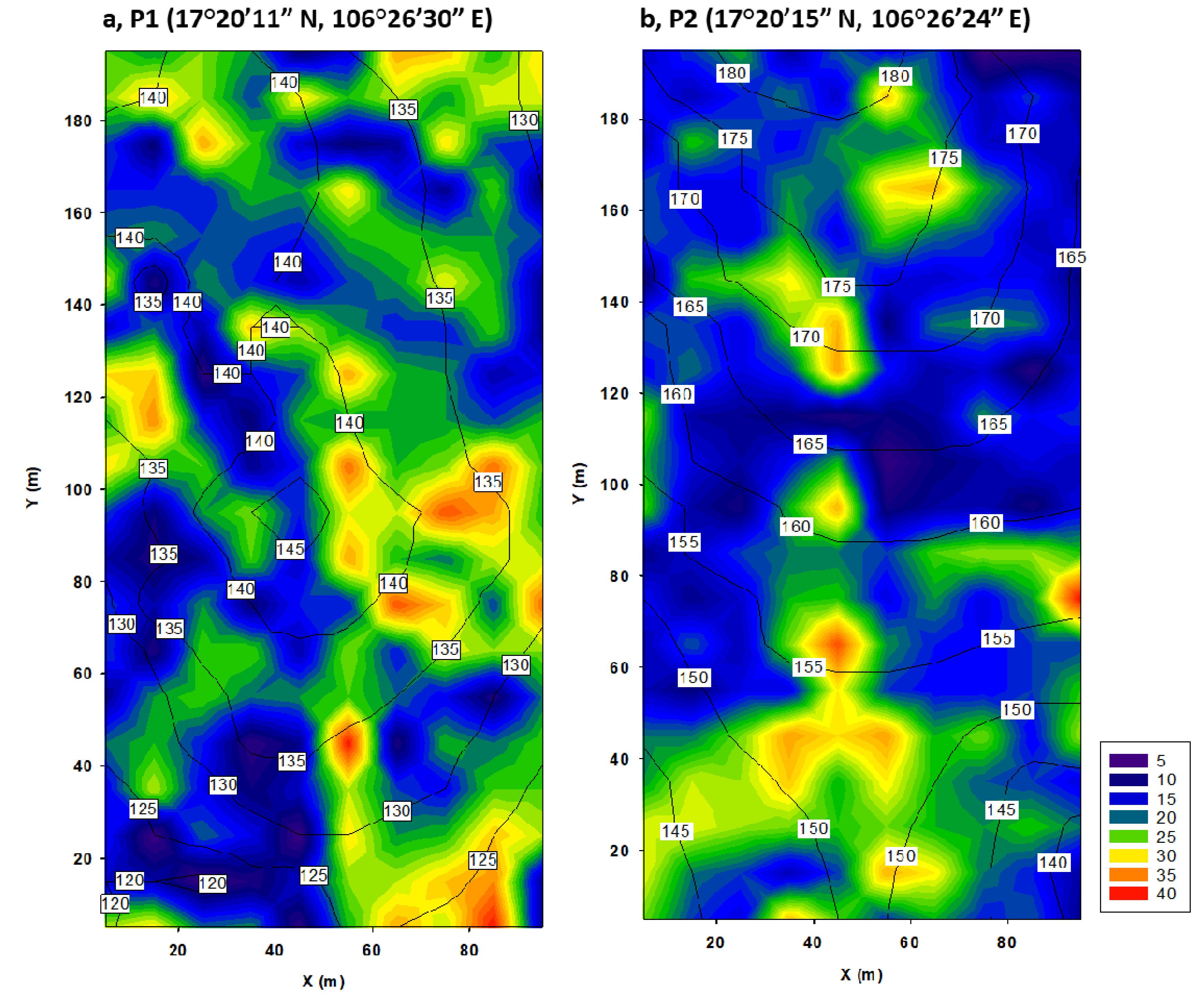
2.1. Study Site and Data Collection

The study plots were located in tropical evergreen broadleaf forests in North Central Vietnam (Figure 1). The climate regime of the study region is characterized as tropical monsoon, since the average annual temperature and the average annual precipitation are 23.5 °C and 3000 mm, respectively. In general, almost 60% to 70% of the annual precipitation falls in autumn (from October to November), while the dry season happens in spring and summer (from March to August).
The study plots of 100 × 200 m (Figure 2), P1 (17°20′11″ N, 106°26′30″ E) and P2 (17°20′15″ N, 106°26′24″ E) recorded by Garmin 60 s GPS (Global Positioning System) using WGS-84 datum at the center of the plots, were designed and subdivided into two grid systems of 200 (10 × 10 m) subplots for measuring tree individuals and topographic data. Slope of the plots ranges from 5 to 45 degrees with an elevation ranging from 119 to 184 m above sea level [26]. Tree individuals with dbh (diameter at breast height) ≥ 2.5 cm were stem-mapped within the plots and their biophysical characteristics (i.e., species type and dbh) were recorded. Canopy cover was recorded at the center of every subplot by taking hemispherical photographs of subplot canopy and assessed by the Gap light analysis mobile application [27]. The topographic variables (i.e., slope and aspect) and relative tree positions (x, y) were recorded in each subplot using a laser distance meter (Leica Disto D2) and compass. Elevation was firstly recorded by Garmin 60 s GPS at the lower left corner of the plot and then calculated by inclinometer for other corners within each subplot and registered as the mean of the elevation. This forest area was certified for sustainable forest management in 2011, so it has been well-protected for decades.

2.2. Data Analysis

2.2.1. Community Properties

Commonly used taxonomic diversity indices including species richness, Shannon, Pielou evenness, and Simpson indices of entropy were calculated within each subplot [28] as follows:
Species richness (S) is number of observed species.
Shannon index (H) = −∑pi lnpi, where pi = ni/N, i = 1 to S, ni is number of individuals of species I, N is total number of individuals.
Pielou index (J) = H/logS.
Simpson index (1−D) = 1 − ∑pi2.
Species richness is defined as the actual number of species present in each subplot; however, the Simpson index is related to the abundance of species. The Shannon index, describing the disorder and uncertainty of individual species, is particularly sensitive to the number of rare species within the study area, while the Simpson index [29] reflects the number of abundant species [30]. The diversity indices were calculated for each subplot by PAST ver. 3.25 software (Paleontological Statistics, https://folk.uio.no/ohammer/past/, accessed on 1 December 2020). Additionally, the AGB (above-ground biomass) of all species individuals was assessed by the allometric equation obtained by Chave et al. [31] for evergreen broadleaf forests: AGB = 0.12843 × D2.409076, where D is dbh (cm).
Differences between the two plots (sites) in structural traits (species richness, abundance, Simpson index, Shannon index, Evenness, Canopy cover, Basal area, AGB) and in topographical parameters (slope, altitude, and aspect) were tested by one-way analysis of variance (ANOVA) considering plots as factors (categorical variable). If the ANOVA provides us with a significant site effect (F-test, p < 0.05), the differences in structural traits between both plots are examined by the Scheffe post hoc test. Prior to the ANOVA, the Kolmogorov–Smirnov and Levene’s tests were performed to assess normality of residuals and homoscedasticity of variance, respectively. If the data did not comply with the requirements of parametric tests (i.e., heteroscedasticity of variance, p < 0.05 in Levene’s test), the differences of the plots were examined by the non-parametric Mann–Whitney U test.

2.2.2. Topographical Effects on Community Properties

The difference in biotic characteristics between the plots under heterogeneous topographic environment was examined, including number of species individuals, abundance, basal area, and AGB, and species diversity indices (i.e., Simpson, Shannon, and Evenness) and topographic variables (i.e., elevation, slope, and aspect) by non-metric multi-dimensional scaling (NMDS), using abundance-based Bray-Curtis dissimilarity matrices (adjustment no-share = 0.1; number of permutations = 999). The R software ver. 3.5.1 [32] and the package vegan ver. 2.4–5 [33] were used. To get insights into topographical–community pattern relations, we fitted topographical factors onto NMDS ordinations using the envfit function in the vegan package, and goodness of fit and p-value were permuted 999 times. In addition, species richness, Shannon, Simpson, and Evenness indices were fitted to NMDS ordinations to test whether these individual variables were associated with community patterns.

2.2.3. Overall Species–Species Associations

The interspecific interactions of species within two study plots were compared by the classification scheme proposed by Wiegand et al. [14]. The classification scheme may provide valuable information about species coexistence in species-rich communities. We employed this approach to explore the effects of environmental heterogeneity on biotic interactions of the same species within two study plots as the scheme can be used to study first-order effects due to habitat heterogeneity on species associations. Interspecific associations were classified into four schemes based on the bivariate forms of K-function, K12(r), and the nearest neighbor distribution function, D12(r) [4,20]. The K-function, K12(r), is the bivariate Ripley’s function [34]. The D12(r) is the cumulative nearest neighbor distribution function that exhibits the probability that an individual of species 2 is located within distance r of an individual of species 1. We used a null model in which the spatial location of individuals of focal species were remained unchanged while individuals of species 2 were arranged randomly and independently from the spatial locations of individuals of species 1 [35]. The expectations of the summary statistics, i.e., K12(r) and D12(r), under the null model result in:
K12(r) = πr2 and D12(r) = (1 − exp(−λ2πr2))
Therefore, the classification scheme with the two axes P ^ r   and   M ^ r   were defined as:
P ^ r = D ^ 12 r 1 exp λ 2 π r 2 ;   M ^ r = ln K ^ 12 r ln π r 2
The two-dimensional scheme allows identifying four fundamental types of bivariate associations, as explained in Table 1.
Species pairs showing non-significant effects for a spatial distance r in the summary statistics are classified as ‘no association’ and will appear close to the center of the scheme.
To stabilize the variance, a transformation of K12(r), L12(r) = (K12(r)/π)0.5 was used instead of K12(r).
The two summary statistics were generated from 199 simulations by using Programita software (http://programita.org/ accessed on 1 December 2020) with a distance bin of 1 m. The goodness-of-fit test was conducted to evaluate a significant departure of the empirical summary statistics from the null model, at an error rate of 5%. Because of using two summary statistics, Kij(r) and Dij(r), at the same time, the rank larger than 195 was considered to be significant.

3. Results

In total, 3732 and 3698 tree individuals of 61 and 52 species were recorded in P1 and P2, respectively. Both plots shared 47 identical species, and the most abundant species were Ormosia balansae (Fabaceae), Garuga pierrei and Bursera tonkinensis (Burseraceae), Tarrietia javanica (Malvaceae), Paviesia annamensis (Sapindaceae), and Litsea glutinosa (Lauraceae) (Appendix A).

3.1. Community Properties

The null hypothesis of homoscedasticity of variances was rejected for Species richness, Abundance, Total basal area, Canopy cover, Elevation, Aspect, and AGB (p < 0.05, Levene test, Table 2), and therefore the effect of site/plot on these parameters was tested by applying of non-parametric U test. The structural traits Abundance and Canopy cover were found to be higher in P1 compared to P2, whereas Total basal area, AGB, and Elevation showed the opposite (Table 2). Species richness and Aspect did not vary significantly between plots. In the case of the other tested parameters (Simpson, Shannon, Evenness, and Slope), the null hypothesis of homoscedasticity of variances was accepted and consequently, we were allowed to apply the Scheffe post hoc test. For all three diversity indices (Simpson, Shannon, and Evenness), but also for slope, the mean values of P2 were significantly higher than those of P1 (p < 0.05, Scheffe test, Table 2).

3.2. Effects of Topography on Community Properties

The NMDS ordination (Figure 3) showed that community compositions in the two study plots were significantly influenced by topographical variables (details in Appendix B). In P1 (Figure 3a), the NMDS plot indicated three topographical variables, including slope (R2 = 0.05, p = 0.006), elevation (R2 = 0.06, p = 0.004), and aspect (R2 = 0.03, p = 0.04), significantly affecting community composition. The two topographical variables, elevation and slope, appeared to be positively associated with Abundance (R2 = 0.20, p = 0.001) and Shannon index (R2 = 0.12, p = 0.001), while Aspect was positively associated with Evenness (R2 = 0.27, p = 0.001). Other properties including AGB, Basal area, and Canopy cover were not significantly associated with any topographical variable (p > 0.05).
Interestingly, in P2 (Figure 3b), Slope (R2 = 0.11, p = 0.001) showed a strong correlation with Evenness (R2 = 0.07, p = 0.001). Although Aspect (R2 = 0.0007, p = 0.93) significantly affected Community composition, this topographical variable did not show any relationship with the examined community properties. Similarly to P1, AGB, Basal area, and Canopy cover did not have any links with topographical variables.

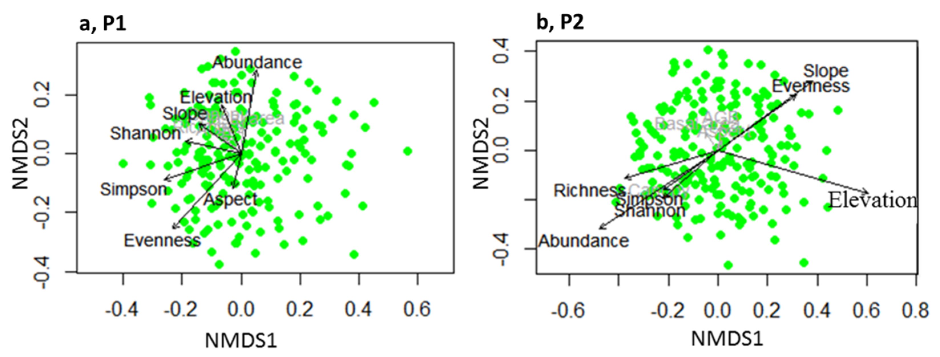
3.3. Overall Species–Species Associations

In total, 420 species pairs of 20 most abundant species with more than 50 individuals in P1 and P2 (Appendix A) were analyzed. The associations of the same heterospecific pairs were influenced by environmental heterogeneity. For example, Tarrietia javanica and Mallotus paniculatus showed spatial segregation in P1 (Figure 4c), which means that individuals of M. paniculatus occurred consistently less around individuals of T. javanica at spatial scales of 0–10 m, however, these two species showed partial overlap in P2 (Figure 4f). Individuals of M. paniculatus occurred more often within neighborhoods (up to 10 m distance) of T. javanica, while a notable proportion of T. javanica on average has less individuals of M. paniculatus as their neighbors. Additionally, T. javanica and Bursera tonkinensis were spatially mixed in P1 (Figure 4e). Individuals of B. tonkinensis were observed around individuals of T. javanica more than expected, at a 0–10 m distance, while they were independently distributed in P2 (Figure 4h), which means that the individuals of the species were not spatially associated.
The overall interspecific interactions of tree species up to scales of 50 m showed that independence patterns were the most dominant association type of tree species and were similar in both study plots, >50% in P1 and 49% in P2, of species pairs (Figure 5). Significant patterns increased with increasing distances up to 10 m, then declined and disappeared at distances larger than 30 m in P1 and 40 m in P2 (Figure 5). Partial overlapping and segregation were the dominant association types in P1, while they were shuffled in P2. In addition, we observed less spatial mixing of tree species in P1 compared to P2, although clustering of species (type IV) was not significantly different in both plots.
The results showed that species segregations were higher in proportion and peaked at 10 m, with 119 species pairs (28%) in P1 compared to 65 species pairs (15%) in P2. Partial overlap of species association increased, and the highest proportion was observed at neighborhoods of 13 m with 82 pairs (19%), then decreased. Partial overlap in P2 (127 pairs, 30%) was at higher proportion and lasted to larger spatial scales, up to 40 m compared to 30 m in P1. Species mixing was found at a lower proportion of 0.14 in P1 (61 pairs, 14%) and decreased to low proportions at spatial scales of 30 m, while it peaked at a proportion of 0.18 (75 pairs, 17%) and remained stable up to large scales of 50 m in P2. No associations (type IV) were dominant at very low proportions up to large scales of 50 m in both study plots (Figure 5). In general, environmental heterogeneity in P2 could increase extreme cases of partial overlap, decrease segregation, and retain the spatial patterns at larger scales compared to that in P1.

4. Discussion

Our results showed significant effects of topographic heterogeneity on community composition and species associations. Species diversity and community structure strongly correlated with the topographic variables, i.e., Elevation, Slope, and Aspect. Interspecific associations such as spatial segregation, partial overlap, and mixing were dominant interaction types at small spatial scales up to 30 m, while the effects of habitat heterogeneity occurred at larger scales.

4.1. Topographical Effects on Community Properties

The association of plant species and their habitats have long been investigated by correlating indices of local properties and habitat variables [6,17,36,37]. Species–habitat associations at large scales caused by biophysical gradients have been observed in tropical forests such as altitudinal zones [38], meso-scales of 1–50 ha [6,36], and landscape scales [39], while investigations at small scales have recently been receiving attention [40,41]. Our analyses using 10 × 10 m quadrats for measures of topographic variables and individual tree locations show that microhabitat differentiation and microhabitat–species association also exist at this fine scale.
A better understanding of the relationship between spatial changes in environmental conditions and the underlying physiological processes may be explored by comparison of demographic rates according to habitat characteristics [42]. However, the degree to which variation in species spatial distribution is explained by topographic variation is negligible. For example, Guo et al. [41] found 16.7% of the total variance in species abundance combining with seven topographical variables including elevation, slope, convexity, slope, rock-bareness rate, topographical wetness index, and altitude above channel at a spatial scale of 10 × 10 m in a 15 ha study area in tropical karst seasonal rainforests, China. The authors emphasized the overall strong evidence of topography on spatial species patterns and a negligible effect of spatially independent habitat. In another 20 ha study area within tropical rainforests in Xishuangbanna, China, Lan et al. [43] also found strong evidence for the effects of topographic variables on species distribution; however, topographic variables explained a small proportion of the observed variation. Moreover, Liu et al. [44] explored significant changes of species composition and mixture along the topographical gradient within the similar forests.

4.2. Overall Species–Species Associations

The most significant interactions between tree species occurred in their neighborhood spatial scales, as spacing between heterospecifics was closely related to coexistence mechanisms [22,23,45]. In our study, approximately 50% of species pairs showed significant interactions: the percentage of species pairs having significant interactions increased with increasing spatial scales up to 10–15 m, then declined and disappeared at larger scales of 30–40 m. Segregation and partial overlap were the dominant association types and decreased with increasing distances up to 30–50 m in our study plots.
In a 25 ha study area in tropical dipterocarp forests of Sri Lanka, Wiegand et al. [14] found that a significant neighborhood of plant interactions occurred within small spatial scales (i.e., 2–4 m) and disappeared within scales of 15–20 m from the focal plant individuals. Moreover, among interspecific associations of 46 species, approximately 50.2% showed segregation, 5.4% mixing, and 34% partial overlap. Wang et al. [46] analyzed 15 common species associations in a 25 ha temperate forest of Changbaishan, China, and found 54.8% of segregation in small scales up to 15 m, 20% of partial overlap, and 6.2% of mixing. Positive associations were rare in local neighborhoods and only 8% of species pairs co-occurred at large spatial scales. In addition, Velázquez et al. [47] explored that almost 50% of the 64 species pairs showed no significant associations and strong positive spatial patterns occurred in spatial scales of 5 and 30 m and negative patterns in a 5 m neighborhood within a 50 ha study plot in tropical forests at Barro Colorado Island. These studies lend support for the significant effects of environmental heterogeneity on species interaction and suggest that the tendency of species segregation may be a supplementary effect of processes promoting species coexistence [14], evidences of competitive interaction among species [46,48], or topographic habitat preference-related species associations at small and large scales [47]. Wiegand et al. [4] examined the independence of tree species associations from three large study plots in tropical forests with high biodiversity at Barro Colorado Island (Panama), tropical dipterocarp forests at Sinharaja (Sri Lanka), and temperate forests at Changbaishan (China). The authors found no significant heterospecific association that was increased with species richness; however, segregation and small-scale interaction of heterospecifics were decreased with species richness. They suggested that independence may be the dominant association type in communities with high biodiversity. Our findings are in line with those mentioned above as well as other studies (e.g., Nguyen et al. [26], Zhou et al. [48]) using the approach of classification scheme for association patterns of tree species.
In this study, we found that partial overlapping and segregation dominate the entire species association at small spatial scales. The spatial segregation is hypothesized as a mechanism that reduces the possibility of encounters shaping highly diverse communities and facilitates species coexistence [49], which is maintained by the balanced extent of intra- and inter-specific competitions [22,23]. If aggregated patterns of conspecifics cause segregation of other species from clusters, it can be inferred that the intraspecific competition is more important than the interspecific competition, resulting in enhancement of species coexistence [4,49]. Moreover, the species herd protection hypothesizes that interspecific neighborhood can promote co-existence of species by biological mechanisms such as preventing biotic plant pests to be transmitted, therefore increasing positive interactions between species [7,50]. Spatial segregation may also be a result of environmental heterogeneity in which a negative association of species individuals can be observed if the two species show dissimilarity in habitat preferences [4]. Zhou et al. [48] argued that interspecific spatial patterns generate spatial segregation and partial overlap under habitat heterogeneity, in addition, frequently negative associations might be a result of resource competition. Our results suggest that aggregation of conspecifics may not be strong enough to shape local dominance and provide evidence of the reduction of species richness according to aggregation of conspecifics and segregation of heterospecifics that comply with previous studies in species-rich communities [4,23,45,51].

5. Conclusions

Our analyses revealed that environmental heterogeneity remained the important driver in maintaining species associations in species-rich forest communities. Spatial segregation, partial overlap, and mixing were displayed at different frequencies and spatial scales smaller than 30 m of species associations. Here, topographical variables such as Elevation, Slope, and Aspect were the main drivers of habitat heterogeneity. These findings remain for future research to explore the above- and below-ground factors to aid understanding of the underlying processes which structure species patterns, particularly for purposes of sustainable forest management with appropriate silvicultural interventions. Based on our results, we can identify topographically heterogeneous parts of tropical forest stands and concentrate management activities (e.g., thinning) to these areas to prevent species’ natural removal, facilitate natural regeneration of focal species, maintain species composition, and/or increase diversity. Though widely applied in forest ecology studies, the approach of spatial point pattern analysis is often costly and time-consuming because of a prerequisite for the stem-mapped data, especially in large plots. However, the applied approach used in this study may be an important scientific tool for decision-makers involved in forest management planning in a sustainable way, even in the case of heterogeneous, tropical, species-rich forests.

Author Contributions

N.H.H. and T.H.M. conceived/designed the experiment and collected the data; N.H.H., Y.E., V.B.B., and I.C.P. analyzed the data; N.H.H., Y.E., V.B.B., T.H.M., and I.C.P. wrote the paper; A.M.P. designed the study map and revised the paper. All authors have read and agreed to the published version of the manuscript.

Funding

This research is funded by Vietnam National Foundation for Science and Technology Development (NAFOSTED) under grant number 106.06-2019.307.

Institutional Review Board Statement

Not applicable.

Informed Consent Statement

Not applicable.

Data Availability Statement

Data supporting this study are available on request to the first author.

Acknowledgments

We thank the three anonymous reviewers and the editor for the constructive comments and suggestions that improved the previous draft of our manuscript.

Conflicts of Interest

The authors declare no conflict of interest.

Appendix A

Table A1. Characteristics of Most Abundant Species in P1 and P2.
NoTree SpeciesP1P2Shade Tolerance
NDBH (cm) IVI (%)NDBH (cm)IVI (%)
1Garuga pierrei28210.08 ± 10.898.9823211.30 ± 13.267.72Tolerant
2Tarrietia javanica3835.62 ± 6.397.283304.52 ± 3.585.14Intolerant
3Ormosia balansae13817.05 ± 12.977.2618714.75 ± 10.816.60Intolerant
4Bursera tonkinensis3846.15 ± 4.166.722536.67 ± 4.124.41Medium
5Paviesia annamensis2409.18 ± 7.646.022396.94 ± 4.864.32Intolerant
6Litsea glutinosa2298.06 ± 6.214.962648.26 ± 6.705.49Intolerant
7Castanopsis indica16810.21 ± 8.274.65-- Intolerant
8Polyalthia nemoralis3035.02 ± 1.774.582445.53 ± 1.883.78Intolerant
9Syzygium wightianum1799.36 ± 7.044.408111.56 ± 8.171.54Intolerant
10Erythrophfloeum fordii6318.52 ± 15.353.96---Medium
11Mallotus kurzii2654.01 ± 0.983.761143.71 ± 0.731.63Intolerant
12Amoora dasyclada1487.99 ± 6.733.28968.89 ± 6.932.08Medium
13Cinnamomun bejolghota10010.71 ± 9.253.0026713.01 ± 10.598.51Intolerant
14Gironniera Subaequalis929.71 ± 6.652.2713711.19 ± 9.283.73Medium
15Endosperrmun sinensis5411.77 ± 13.182.148321.67 ± 13.334.63Intolerant
16Garcinia oblongifolia1216.23 ± 4.082.11676.22 ± 3.481.11Tolerant
17Canarium album---15511.03 ± 6.043.68Intolerant
18Koilodepas hainanense1045.83 ± 2.611.68808.41 ± 4.521.54Tolerant
19Cassine glauca748.41 ± 5.511.59898.69 ± 7.661.97Tolerant
20Litsea vang716.54 ± 3.301.27768.72 ± 4.671.5Intolerant
21Symplocos laurina559.31 ± 5.611.2514511.81 ± 6.863.71Intolerant
22Engelhardtia roxburghiana-- 6328.78 ± 11.914.84Tolerant
N—Number of individuals, IVI—Important Value Index, (relative abundance + relative basal area)/2, expressed as percentage proportion. DBH—Diameter at Breast Height (mean ± standard deviation).

Appendix B

Table A2. NMDS Ordination of the Compositional Structures with Topography in P1 and P2.
PropertiesPlot P1Plot P2
NMDS1NMDS2r2Pr (>r)NMDS1NMDS2r2Pr (>r)
Richness−0.84966−0.527330.04120.016 −0.95625−0.292560.07750.001
Abundance0.08552−0.996340.20510.001 −0.82451−0.565840.16770.001
Canopy cover−0.57273−0.819740.02920.051−0.8942−0.447660.0170.171
Basal area0.01327−0.999910.02040.159−0.330530.94380.00470.678
Simpson−0.957270.289190.19980.001 −0.82216−0.569260.03790.025
Shannon−0.97059−0.240740.11940.001 −0.76235−0.647160.04440.009
Evenness−0.654680.75590.27730.001 0.807350.590070.07310.001
AGB−0.76702−0.641630.01210.3150.215480.976510.00850.457
Elevation−0.25379−0.967260.06340.004 0.96418−0.265240.21720.001
Slope−0.81517−0.579220.05720.006 0.809280.587430.11880.001
Aspect−0.242810.970070.0330.04 −0.104310.994540.00070.927
NMDS1 and NMDS2: Non-metric multidimensional scaling axes, r: proportion, Pr: significance.

References

  1. Chesson, P. Mechanisms of maintenance of species diversity. Annu. Rev. Ecol. Syst. 2000, 31, 343–366. [Google Scholar] [CrossRef] [Green Version]
  2. Wright, J.S. Plant diversity in tropical forests: A review of mechanisms of species coexistence. Oecologia 2002, 130, 1–14. [Google Scholar] [CrossRef]
  3. May, F.; Huth, A.; Wiegand, T. Moving beyond abundance distributions: Neutral theory and spatial patterns in a tropical forest. Proc. R. Soc. B Biol. Sci. 2015, 282, 20141657. [Google Scholar] [CrossRef]
  4. Wiegand, T.; Huth, A.; Getzin, S.; Wang, X.; Hao, Z.; Gunatilleke, C.S.; Gunatilleke, I.N. Testing the independent species’ arrangement assertion made by theories of stochastic geometry of biodiversity. Proc. R. Soc. B. 2012, 279, 3312–3320. [Google Scholar] [CrossRef] [Green Version]
  5. Volkov, I.; Banavar, J.R.; Hubbell, S.P.; Maritan, A. Inferring species interactions in tropical forests. Proc. Natl. Acad. Sci. USA 2009, 106, 13854–13859. [Google Scholar] [CrossRef] [PubMed] [Green Version]
  6. Harms, K.E.; Condit, R.; Hubbell, S.P.; Foster, R.B. Habitat associations of trees and shrubs in a 50-ha neotropical forest plot. J. Ecol. 2001, 89, 947–959. [Google Scholar] [CrossRef]
  7. Nguyen, H.H.; Uria-Diez, J.; Wiegand, K. Spatial distribution and association patterns in a tropical evergreen broad-leaved forest of north-central Vietnam. J. Veg. Sci. 2016, 27, 318–327. [Google Scholar] [CrossRef]
  8. May, F.; Giladi, I.; Ziv, Y.; Jeltsch, F. Dispersal and diversity–unifying scale-dependent relationships within the neutral theory. Oikos 2012, 121, 942–951. [Google Scholar] [CrossRef]
  9. Adler, P.B.; Fajardo, A.; Kleinhesselink, A.R.; Kraft, N.J. Trait-based tests of coexistence mechanisms. Ecol. Lett. 2013, 16, 1294–1306. [Google Scholar] [CrossRef]
  10. Shipley, B.; Paine, C.T.; Baraloto, C. Quantifying the importance of local niche-based and stochastic processes to tropical tree community assembly. Ecology 2012, 93, 760–769. [Google Scholar] [CrossRef] [Green Version]
  11. Kraft, N.J.; Ackerly, D.D. Functional trait and phylogenetic tests of community assembly across spatial scales in an Amazonian forest. Ecol. Monogr. 2010, 80, 401–422. [Google Scholar] [CrossRef]
  12. Hubbell, S.P.; Ahumada, J.A.; Condit, R.; Foster, R.B. Local neighborhood effects on long-term survival of individual trees in a neotropical forest. Ecol. Res. 2001, 16, 859–875. [Google Scholar] [CrossRef]
  13. Uriarte, M.; Condit, R.; Canham, C.D.; Hubbell, S.P. A spatially explicit model of sapling growth in a tropical forest: Does the identity of neighbours matter? J. Ecol. 2004, 92, 348–360. [Google Scholar] [CrossRef]
  14. Wiegand, T.; Gunatilleke, S.; Gunatilleke, N. Species associations in a heterogeneous Sri lankan dipterocarp forest. Am. Nat. 2007, 170, E77–E95. [Google Scholar] [CrossRef] [Green Version]
  15. Lan, G.; Getzin, S.; Wiegand, T.; Hu, Y.; Xie, G.; Zhu, H.; Cao, M. Spatial Distribution and Interspecific Associations of Tree Species in a Tropical Seasonal Rain Forest of China. PLoS ONE 2012, 7, e46074. [Google Scholar] [CrossRef]
  16. Aiba, S.; Kitayama, K.; Takyu, M. Habitat associations with topography and canopy structure of tree species in a tropical montane forest on Mount Kinabalu, Borneo. Plant Ecol. 2004, 174, 147–161. [Google Scholar] [CrossRef]
  17. Punchi-Manage, R.; Wiegand, T.; Wiegand, K.; Getzin, S.; Gunatilleke, C.S.; Gunatilleke, I.N. Effect of spatial processes and topography on structuring species assemblages in a Sri Lankan dipterocarp forest. Ecology 2014, 95, 376–386. [Google Scholar] [CrossRef]
  18. Lai, J.; Mi, X.; Ren, H.; Ma, K. Species-habitat associations change in a subtropical forest of China. J. Veg. Sci. 2009, 20, 415–423. [Google Scholar] [CrossRef]
  19. Illian, J.; Penttinen, A.; Stoyan, H.; Stoyan, D. Statistical Analysis and Modelling of Spatial Point Patterns; John Wiley & Sons: Hoboken, NJ, USA, 2008; Volume 70. [Google Scholar]
  20. Wiegand, T.; Moloney, K.A. Handbook of Spatial Point-Pattern Analysis in Ecology; CRC Press: Boca Raton, FL, USA, 2014. [Google Scholar]
  21. Law, R.; Illian, J.; Burslem, D.F.; Gratzer, G.; Gunatilleke, C.V.S.; Gunatilleke, I.A.U.N. Ecological information from spatial patterns of plants: Insights from point process theory. J. Ecol. 2009, 97, 616–628. [Google Scholar] [CrossRef]
  22. Pacala, S.W.; Levin, S.A. Biologically generated spatial pattern and the coexistence of competing species. In Spatial Ecology: The Role of Space in Population Dynamics and Interspecific Interactions; Princeton University Press: Princeton, NJ, USA, 1997; pp. 204–232. [Google Scholar]
  23. Stoll, P.; Prati, D. Intraspecific aggregation alters competitive interactions in experimental plant communities. Ecology 2001, 82, 319–327. [Google Scholar] [CrossRef]
  24. McGill, B.J. Towards a unification of unified theories of biodiversity. Ecol. Lett. 2010, 13, 627–642. [Google Scholar] [CrossRef] [PubMed]
  25. Getzin, S.; Wiegand, T.; Wiegand, K.; He, F. Heterogeneity influences spatial patterns and demographics in forest stands. J. Ecol. 2008, 96, 807–820. [Google Scholar] [CrossRef]
  26. Nguyen, H.H.; Erfanifard, Y.; Pham, V.D.; Le, X.T.; Petritan, I.C. Spatial Association and Diversity of Dominant Tree Species in Tropical Rainforest, Vietnam. Forests 2018, 9, 615. [Google Scholar] [CrossRef] [Green Version]
  27. Tichý, L. Field test of canopy cover estimation by hemispherical photographs taken with a smartphone. J. Veg. Sci. 2016, 27, 427–435. [Google Scholar] [CrossRef]
  28. Magurran, A.E. Ecological Diversity and Its Measurement; Princeton University Press: Princeton, NJ, USA, 1988. [Google Scholar]
  29. Simpson, E.H. Measurement of diversity. Nature 1949, 163, 688. [Google Scholar] [CrossRef]
  30. Heip, C.H.; Herman, P.M.; Soetaert, K. Indices of diversity and evenness. Oceanis 1998, 24, 61–88. [Google Scholar]
  31. Chave, J.; Réjou-Méchain, M.; Búrquez, A.; Chidumayo, E.; Colgan, M.S.; Delitti, W.B.; Duque, A.; Eid, T.; Fearnside, P.M.; Goodman, R.C.; et al. Improved allometric models to estimate the aboveground biomass of tropical trees. Glob. Chang. Biol. 2014, 20, 3177–3190. [Google Scholar] [CrossRef] [PubMed]
  32. Team, R.C. R: A Language and Environment for Statistical Computing; Ver. 3.5. 1; R Foundation for Statistical Computing: Vienna, Austria, 2018. [Google Scholar]
  33. Oksanen, J. Vegan: An Introduction to Ordination. Available online: http://cran.r-project.org/web/packages/vegan/vignettes/introvegan.pdf (accessed on 1 December 2020).
  34. Ripley, B.D. Modelling spatial patterns. J. R. Stat. Soc. Ser. B (Methodol.) 1977, 39, 172–212. [Google Scholar] [CrossRef]
  35. Wiegand, T.; Moloney, K. Rings, circles, and null-models for point pattern analysis in ecology. Oikos 2004, 104, 209–229. [Google Scholar] [CrossRef]
  36. Comita, L.S.; Condit, R.; Hubbell, S.P. Developmental changes in habitat associations of tropical trees. J. Ecol. 2007, 95, 482–492. [Google Scholar] [CrossRef]
  37. Wang, Z.; Ye, W.; Cao, H.; Huang, Z.; Lian, J.; Li, L.; Wei, S.; Sun, I.F. Species–topography association in a species-rich subtropical forest of China. Basic Appl. Ecol. 2009, 10, 648–655. [Google Scholar] [CrossRef]
  38. Gentry, A.H. Changes in plant community diversity and floristic composition on environmental and geographical gradients. Ann. Mo. Bot. Gard. 1988, 1–34. [Google Scholar] [CrossRef]
  39. Paoli, G.D.; Curran, L.M.; Zak, D.R. Soil nutrients and beta diversity in the Bornean Dipterocarpaceae: Evidence for niche partitioning by tropical rain forest trees. J. Ecol. 2006, 94, 157–170. [Google Scholar] [CrossRef] [Green Version]
  40. Prada, C.M.; Stevenson, P.R. Plant composition associated with environmental gradients in tropical montane forests (Cueva de Los Guacharos National Park, Huila, Colombia). Biotropica 2016, 48, 568–576. [Google Scholar] [CrossRef]
  41. Guo, Y.; Wang, B.; Li, D.; Mallik, A.U.; Xiang, W.; Ding, T.; Wen, S.; Lu, S.; Huang, F.; He, Y.; et al. Effects of topography and spatial processes on structuring tree species composition in a diverse heterogeneous tropical karst seasonal rainforest. Flora 2017, 231, 21–28. [Google Scholar] [CrossRef]
  42. Lasky, J.R.; Sun, I.F.; Su, S.H.; Chen, Z.S.; Keitt, T.H. Trait-mediated effects of environmental filtering on tree community dynamics. J. Ecol. 2013, 101, 722–733. [Google Scholar] [CrossRef]
  43. Lan, G.; Hu, Y.; Cao, M.; Zhu, H. Topography related spatial distribution of dominant tree species in a tropical seasonal rain forest in China. For. Ecol. Manag. 2011, 262, 1507–1513. [Google Scholar] [CrossRef]
  44. Liu, J.; Yunhong, T.; Slik, J.F. Topography related habitat associations of tree species traits, composition and diversity in a Chinese tropical forest. For. Ecol. Manag. 2014, 330, 75–81. [Google Scholar] [CrossRef]
  45. Raventós, J.; Wiegand, T.; Luis, M.D. Evidence for the spatial segregation hypothesis: A test with nine-year survivorship data in a Mediterranean shrubland. Ecology 2010, 91, 2110–2120. [Google Scholar] [CrossRef]
  46. Wang, X.; Wiegand, T.; Hao, Z.; Li, B.; Ye, J.; Lin, F. Species associations in an old-growth temperate forest in north-eastern China. J. Ecol. 2010, 98, 674–686. [Google Scholar] [CrossRef]
  47. Velázquez, E.; Paine, C.T.; May, F.; Wiegand, T. Linking trait similarity to interspecific spatial associations in a moist tropical forest. J. Veg. Sci. 2015, 26, 1068–1079. [Google Scholar] [CrossRef]
  48. Zhou, Q.; Shi, H.; Shu, X.; Xie, F.; Zhang, K.; Zhang, Q.; Dang, H. Spatial distribution and interspecific associations in a deciduous broad-leaved forest in north-central China. J. Veg. Sci. 2019, 30, 1153–1163. [Google Scholar] [CrossRef]
  49. Chesson, P. General theory of competitive coexistence in spatially-varying environments. Theor. Popul. Biol. 2000, 58, 211–237. [Google Scholar] [CrossRef] [PubMed]
  50. Peters, H.A. Neighbour-regulated mortality: The influence of positive and negative density dependence on tree populations in species-rich tropical forests. Ecol. Lett. 2003, 6, 757–765. [Google Scholar] [CrossRef] [Green Version]
  51. Pacala, S.W. Dynamics of plant communities. Plant Ecol. 1997, 532–555. [Google Scholar]
Figure 1. Maps of Vietnam, study region and plots.
Sustainability 13 02468 g001
Figure 2. Contour maps of tree density and elevation in the two 2-ha plots P1 (a) and P2 (b). Colors indicate tree density of subplots. Contours show 5 m intervals of elevation.
Sustainability 13 02468 g002
Figure 3. NMDS ordination showed the effects of topographical variables on the compositional structure of the forest plots: P1 (a) and P2 (b) with stress value = 0.09. The significant variables (p < 0.05) were displayed in black arrows and non-significant variables (p > 0.05) in grey.
Sustainability 13 02468 g003
Figure 4. Classification of species–species associations at the two study plots. Overall species associations of 420 species pairs were allocated based on P(r) and M(r) at small spatial scale (0–10 m) (a, b) and large spatial scale (0–30 m) (i, j) in P1 and P2. The grey circles indicated significant species–species association types, while red circles showed no significant departure from the null model of independence. Examples: (c) Segregation: T. javanica vs. M. paniculatus in P1. (d) Partial overlap: T. javanica vs. P. annamensis in P1. (e) Mixing: T. javanica vs. B. tonkinensis in P1. (f) Segregation: T. javanica vs. M. paniculatus in P1 changed to partial overlapping in P2. (g) Partial overlapping: T. javanica vs. P. annamensis in P1 turned to independence in P2. (h) Independence: T. javanica vs. B. tonkinensis in P2 that were mixed in P1. In panels (ch), black dots are the focal species (=i, i.e., T. javanica) and red dots are secondary species (=j).
Sustainability 13 02468 g004
Figure 5. The overall interspecific associations of 20 species and their spatial scale-dependences in P1 (a) and P2 (b).
Sustainability 13 02468 g005
Table 1. The types of association identified by the classification scheme.
Type of AssociationFunction
Segregation (i.e., less individuals of species 2 on average around species 1 than expected by chance) M ^ r < 0   and   P ^ r < 0
Partial overlap (i.e., frequent individuals of species 2 around some individuals of species 1, despite others) M ^ r > 0   and   P ^ r < 0
Mixing (i.e., frequent individuals of species 2 around individuals of species 1) M ^ r > 0   and   P ^ r > 0
Type IV (i.e., overlapping of individuals of species 2 on dense cluster of individuals of species 1 and 2) M ^ r 0   and   P ^ r 0
Table 2. Basic description of the two study plots.
Characteristics
(Mean ± SD)
P1P2p-Value for the Test
Levene’sPost Hoc ScheffeMann–Whitney
Elevation (m)134.30 ± 6.32 a160.67 ± 11.09 b<0.001 <0.001
Slope (°)20.22 ± 6.61 a26.6 ± 7.54 b0.203<0.001
Aspect (°)87.51 ± 55.46 a91.08 ± 47.96 a<0.001 0.413
Species richness11.39 ± 2.38 a11.48 ± 2.68 a0.013 0.533
Abundance19.67 ± 5.19 a18.69 ± 6.35 b0.018 0.025
Canopy cover (%)83.38 ± 4.52 a81.01 ± 7.37 b<0.001 <0.001
Shannon index2.22 ± 0.36 a2.29 ± 0.29 b0.6050.035
Simpson index0.87 ± 0.04 a0.88 ± 0.03 b0.2580.024
Evenness index0.85 ± 0.07 a0.88 ± 0.06 b0.3910.002
Total basal area (m2)0.24 ± 0.15 a0.32 ± 0.18 b<0.001 <0.001
AGB (Mg)1559.27 ± 1406.18 a2152.42 ± 1545.60 b0.005 <0.001
Values for a parameter marked by different letters differ significantly (p < 0.05). SD- standard deviation
Publisher’s Note: MDPI stays neutral with regard to jurisdictional claims in published maps and institutional affiliations.

