Machine Learning Based Short-Term Travel Time Prediction: Numerical Results and Comparative Analyses

Abstract

Due to the increasing traffic volume in metropolitan areas, short-term travel time prediction (TTP) can be an important and useful tool for both travelers and traffic management. Accurate and reliable short-term travel time prediction can greatly help vehicle routing and congestion mitigation. One of the most challenging tasks in TTP is developing and selecting the most appropriate prediction algorithm using the available data. In this study, the travel time data was provided and collected from the Regional Integrated Transportation Information System (RITIS). Then, the travel times were predicted for short horizons (ranging from 15 to 60 min) on the selected freeway corridors by applying four different machine learning algorithms, which are Decision Trees (DT), Random Forest (RF), Extreme Gradient Boosting (XGBoost), and Long Short-Term Memory neural network (LSTM). Many spatial and temporal characteristics that may affect travel time were used when developing the models. The performance of prediction accuracy and reliability are compared. Numerical results suggest that RF can achieve a better prediction performance result than any of the other methods not only in accuracy but also with stability.

1. Introduction

TTP has important information that travelers rely on increasingly, and meanwhile, it is also essential for transportation agencies and traffic management authorities. Short-term TTP is a key component of the Advanced Travelers Information System (ATIS) in which in-vehicle route guidance systems (RGS) and real-time TTP enable the generation of the shortest path for travelers, which connects the destinations and current locations [1]. Accurate TTP on the future state of traffic enables travelers and transportation agencies to plan their trips and mitigate congestion along with specific road segments (such as rerouting traffic or optimising the signaling time of traffic lights), leading to the overall reduction of total travel time and cost. These measures can also help reduce greenhouse gas emissions, as the CO₂ emission rates in congested conditions can be up to 40% higher than those seen in free-flow conditions [2]. Travel time also can be used as a performance measure to evaluate the utility of investments such as the widening of expressways, subways, and roads. TTP has been an interesting and challenging research area for decades to which many researchers have applied various traditional statistical and machine learning algorithms to improve prediction accuracy and stability. The paper develops different machine learning prediction models and compares their performance based on a case study from the City of Charlotte, North Carolina.

In the field of logistics, TTP for minutes or hours is important for dispatching, e.g., when assigning customers to drivers for the deliveries of food or goods. The objective of this study was to develop a series of dynamic machine learning models that can efficiently predict travel time. An unbiased and low-variance prediction of travel time is the ultimate goal. Different machine learning algorithms have been developed, which include DT, RF, XGBoost, and LSTM. Such TTP models were tested and compared using the probe vehicle-based traffic data for selected road segments (i.e., a freeway corridor in Charlotte, North Carolina) from the RITIS. Mean Absolute Percent Error (MAPE) was selected and used as evaluation and comparison criteria. The advantages and disadvantages of the proposed models are also identified and provided. Finally, the effectiveness and efficiency of the proposed models are discussed.

In the field of TTP, the prediction scheme can be classified into short, medium, and long-term horizons based on the prediction duration. Van Lint (2004) defined short term TTP as horizons ranging from several minutes to 60 min [3], while the long-term TTP horizon can take more than a day. Long-term travel times are typically impacted more by the factors such as weather and congestion conditions [4]. Shen (2008) found that setting a proper TTP horizon is a vital factor in evaluating the performance of TTP models [5]. Furthermore, the road characteristics of signalized streets, arterials or freeways, is another classification method. 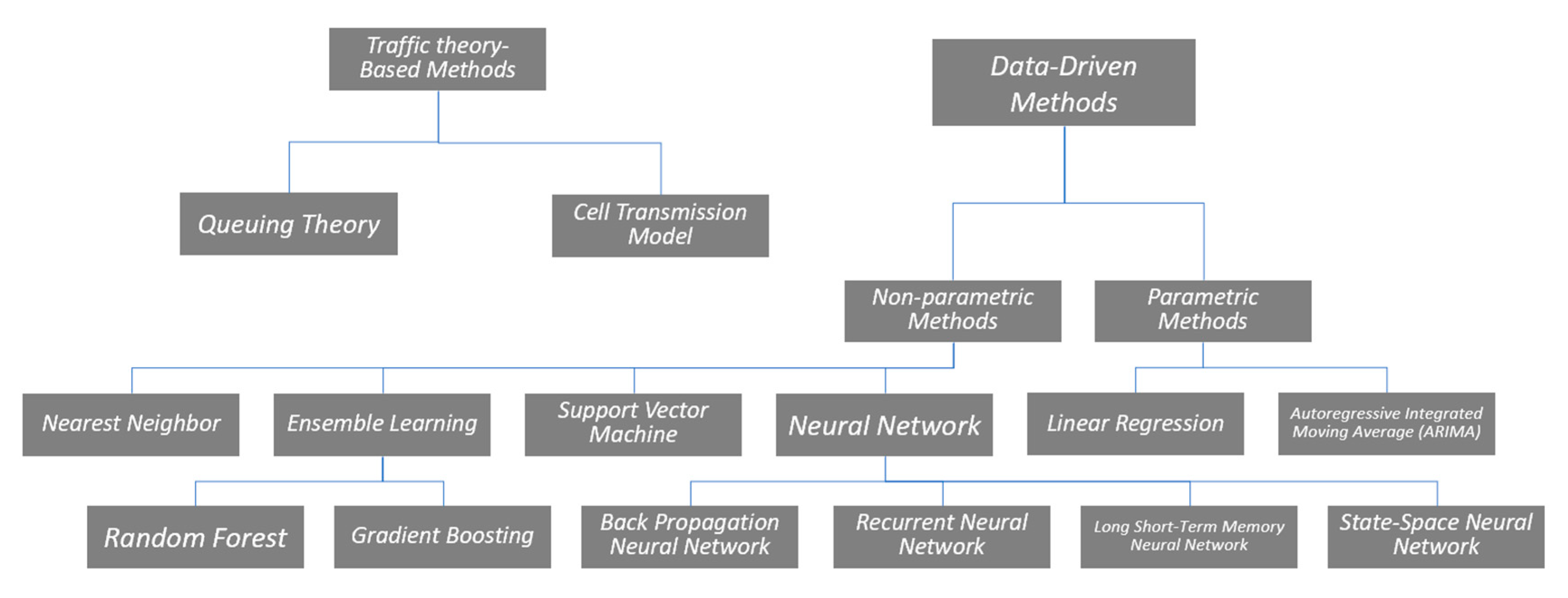Due to additional factors such as signal timing plans and controls at multiple intersections, the TTP on signalized urban roads is inherently more complex than on freeways [6]. The studies have been conducted in the field to develop and improve the accuracy and reliability of TTP, which can generally be classified into traffic theory-based methods and data-based methods. With the rapid development of machine learning methods and the increasing availability of the collected traffic data, data-based methods have become increasingly popular in the last two decades, which can be further divided into two major categories: parametric models and non-parametric models [3]. Parametric methods are model-based methods in which the model structure is predetermined under the specific statistical assumption, and the parameters can be estimated with the sample dataset. Owing to the simplicity of statistical interpretation, the most typical parametric model is linear regression, where the dependent variable is a linear function of the explanatory (independent) input variables. In the TTP, the independent variables are generally traffic factors gathered in several past time intervals. Time series models are another typical type of widely applied parametric model in TTP, where the explanatory variables are a series of data points indexed in the time order. Owing to its statistical principles, the prediction results of the time series model are always highly based on the previously observed values. Autoregressive integrated moving average (ARIMA) model is the most widely used for TTP. The ARIMA model combines two models, which include the autoregressive (AR) and the moving average (MA) models.

Different from parametric models, both the structure and the parameters of the model are not predetermined in the non-parametric models. However, it does not mean that there are no parameters that can be estimated. Instead, the number typology of such parameters is indeterminate or even uncountable. From the taxonomy of the data-driven approach to TTP, the level of model complexity can vary from high to low, from linear regression and time series to artificial intelligence (neural networks, ensemble learning) and pattern searching (nearest neighborhood). The taxonomy of TTP methods is shown in detail in Figure 1.

Benefiting from the rapid development of non-parametric machine learning methods, real-time TTP has become a reality. In the literature of TTP, artificial neural network (ANN) is the most widely used method due to its ability to capture complex relationships in large data sets [7]. ANN is a typical non-parametric model which can be developed without the need to specify the model structure. Therefore, the multicollinearity of the explanatory variables can be overcome to some extent. In the past two decades, researchers in different fields have applied different types of neural networks in the field of traffic prediction using the ANN method (

Table 1. Summary of TTP using machine learning approaches.

Year	Author	Country/City	Data Source	Data Type	Roadway Category	Method Category	Prediction Method
2000	Wunderlich et al.	N/A	Simulated data from INTEGRATION	Travel time	N/A	Navie model	Exponential filtering
2002	Dion et al.	Virginia, US	Simulated data from INTEGRATION	Travel time	N/A	Traffic theory-base model	Delay models
2005	Wu et al.	Taiwan	Loop detector	Travel speed	Highway	Non-parametric	SVR
2007	Schmitt & Jula	California, US	Loop detector	Travel time	Urban road	Navie model	Switch model
2010	Papageorgiou et al.	N/A	simulated data from MATANET	Travel time	N/A	Traffic theory-base model	Macroscopic Simulation
2020	Kwak & Geroliminis	California, US	PeMS	Travel time	Freeway	Parametric	Dynamic linear model
2015	Zhang & Haghani	Maryland, US	INRIX	Travel time	Interstate highway	Non-parametric	Gradient boosting
2016	Li and Bai	Ningbo, China	N/A	Truck trajectory, travel time, travel speed	N/A	Non-parametric	Gradient boosting
2010	Hamner et al.	N/A	GPS	Travel speed	N/A	Non-parametric	RF
2017	Fan et al.	Taiwan	Electric toll	Travel time	Highway	Non-parametric	RF
2018	Gupta et al.	Porto, Portugal	GPS	Taxi travel speed	Urban road	Non-parametric	RF and gradient boosting
2017	Yu et al.	Shenyang, China	AVL system	Bus travel time	Bus route	Non-parametric	RF and KNN
2002	Van Lint et al.	N/A	Simulated data from FOSIM	Travel time, travel speed	Freeway	Non-parametric	State-Space Neural Network
2012	Wisitpongphan	Bangkok, Thailand	GPS	Travel time	Highway	Non-parametric	BP Neural Network
2016	Duan et al.	England	Cameras, GPS and loop detectors	Travel time	Highway	Non-parametric	LSTM Neural Network
2017	Liu et al.	California, US	PeMS	Travel time	Highway	Non-parametric	LSTM Neural Network
2018	Wang et al.	Beijing, China	Floating Car Data	Taxi ravel time, vehicle trajectory data	Urban road	Non-parametric	LSTM Neural Network
2018	Wei et al.	China	Vehicle passage records	Travel time	Urban road	Non-parametric	LSTM Neural Network
2018	Wang et al.	Beijing and Chengdu, China	GPS	Vehicle trajectory data	Urban road	Non-parametric	LSTM Neural Network
2020	Wang et al.	Beijing, China	GISGPS	Travel timeTaxi travel speed	Urban road	Non-parametric	LSTM
2020	Fu et al.	Beijing, Suzhou, Shenyang, China	Ride-hailing platform	Travel time	Urban road	Non-parametric	Graph attention network
2011	Myung et al.	Korea	ATC system	Travel time	N/A	Non-parametric	KNN
2019	Moonam et al.	Madison, Wisconsin, US	Bluetooth detector	Travel speed	Freeway	Non-parametric	KNN
2019	Kumar et al.	Chennai, India	GPS	Travel time	Urban road	Non-parametric	KNN
2019	Cristobal et al.	Gran Canaria, Spain	Public transport network	Travel time	Urban road	Non-parametric	K-Medoid Clustering Technique
2021	Chiabaut & Faitout	Lyon, France	Loop detector	Travel time	Highway	Non-parametric	PCA and Clustering
2008	Zou et al.	Maryland, US	Roadside detector	Travel time	Highway	Hybird non-parametric	Combined Clustering Neural Networks
2009	Li et al.	Atlanta, US	simulated data from VISSIM	Travel time, travel speed	N/A	Hybird non-parametric	Combined Boosting and Neural Network
2013	Yildirimoglu & Geroliminis’s	California, US	Loop detector	Travel time	Freeway	Hybird non-parametric	Combined Gaussian Mixture, PCA, and Clustering
2015	Joao et al.	Porto, Portugal	STCP system	Travel time	Urban road	Hybird non-parametric	Combined RF, Projection Pursuit Regression and SVM

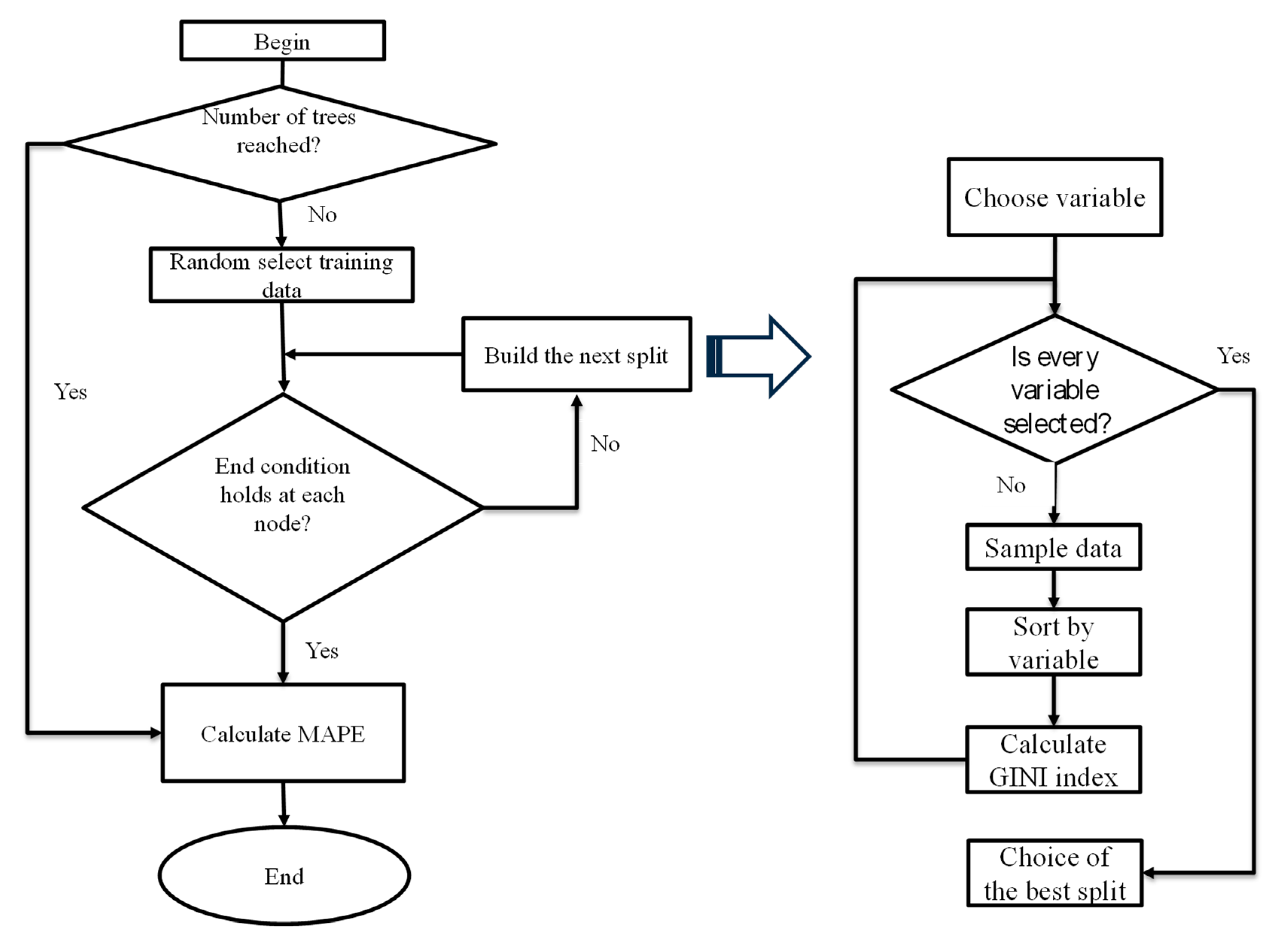
). Park and Rilett used the regular multilayer feedforward neural networks to predict the freeway travel times in Houston, Texas in 1999 [8]. Yildirimoglu and Geroliminis applied spectral basis neural networks to predict the freeway travel time in Los Angeles in California in 2013 [9]. The variables selection is generally a crucial step in machine learning model estimation depending on the data availability and the model training process. In the variable selection, different variations of the backward algorithm consider different types of neural networks. Ensemble tree-based methods are another popular choice for TTP. RF is a tree-based ensemble method, which has become popular in the prediction field. From the name of RF, the forest is made up of separate DTs. Simple DT has ‘poor’ performance, while RFs have a large number of trees that usually produce high prediction accuracy by the swarm intelligence. The gradient boosting machine also combines DTs and starts the combing process at the beginning instead of doing so at the end. Unlike some machine learning methods that work as black-boxes, tree-based ensemble methods can provide more interpretable results and fit complex nonlinear relationships [10].

Support vector machine (SVM) theory was created by Vapnik of AT&T Bell Laboratories [11]. SVM is superior from a theoretical point of view and always performs well in practice [12]. The SVM model is good for TTP based on historical travel time data, and therefore, there are several applications of SVM for TTP [13,14]. Kernel function is the key point in the SVM algorithm, which can map the input data into a higher-dimensional space. The mapping process stops until the flattest linear function is found (i.e., when the error is smaller than a predefined threshold). This linear function was used to map the initial space and obtain the final model, which was used for TTP. However, a crucial problem-overfitting arises from the complicated structure of SVM and ANN algorithms (i.e., the large number of parameters that need to be estimated), which commonly exists in the non-parameter machine learning algorithm.

Another popular non-parametric approach to TTP is the local regression approach. Local linear regression can be used to optimize and balance the use of historical and real time data [15], which can yield accurate prediction results. In the local regression algorithm, a set of historical data with similar characteristics to the current data record are selected by the algorithm.

Semi-parametric models are a combination of specific parametric and non-parametric methods. The main idea of the semi-parametric method is to loosen some of the assumptions created in the parametric model to get a more flexible structure [16]. In the application of TTP, semi-parametric models are always in the form of varying coefficient regression models in which the model coefficient varies depending on the departure time and prediction horizon [17]. Therefore, travel time can be estimated by a linear combination of the naive historical and instantaneous predictors.

With the increasing and wide applications of machine learning algorithms in the field of TTP, mainstream machine learning methods have been deployed in different countries using various types of data sources. Many methodologies have been developed and applied by researchers, which include, but are not limited to, the following: SVM, neural network (e.g., state-and-space neural network, long short-term memory neural network), nearest neighbor algorithm (e.g., k-nearest neighbor), and ensemble learning (e.g., RF and gradient boosting), etc. Nonlinear modelling machine learning methods have also been widely applied and proven successful in many other fields, such as building models for taxi carpooling with simulation [18], predicting the portfolio of stock price affected by the news with multivariate Bayesian structural time series model [19], and evolving fuzzy models for prosthetic hand myoelectric-based control [20]. Table 1 summarizes the studies reviewed that are classified based on the prediction method employed as shown in the last column of the respective studies.

The main innovative idea (and also the main contribution) of this paper is to apply and compare four different machine learning algorithms (i.e., DT, RF, XGBoost, and LSTM) for the TTP. To the authors’ best knowledge, this is the first effort made to systematically develop and compare such four algorithms in the TTP area.

2. Materials and Methods

2.1. Data

2.1.1. Travel Time Data

In this study, the selected freeway segment travel time data were collected from the RITIS. RITIS is an advanced traffic analysis system that includes probe data analytics, segment analysis, and signal analytics. The raw travel data gathered from a series of selected road segments along the I-485 freeway in Charlotte, North Carolina, were used in the case study. As one of the most heavily travelled interstate freeways in the Charlotte metropolitan area, I-485 encircles the city and the last segment was completed in June 2015. The city of Charlotte has experienced a significant increase in daily traffic on many of its freeway segments in the past 25 years as the population of the Charlotte area increased from 688,000 to 1.4 million; more than 500,000 more residents are expected over the next 20 years. Charlotte has the largest population in the state and is also one of the fastest-growing metro areas in the U.S. The rapid population growth has caused traffic congestion on major roads. I-485 freeway segments in the southern Charlotte area experience massive recurrent congestion during weekdays due to heavy commuter and interstate traffic, which can seriously affect the travel and further economic development in this area. The I-485 Express Lanes project that began in the summer of 2019 will be completed in 2022 (the estimated cost is 346 million dollars) with one express lane added in each direction along I-485 between exit 67 (I-77) and exit 51 (U.S. 74). Travel time reliability and traffic flow in these freeway segments are therefore expected to improve. Figure 2 shows the satellite map of the selected sections.

In this study, the selected section of the I-485 southern loop in the RITIS system includes clockwise and counter-clockwise directions and consists of 37 miles of roadways and 32 Traffic Message Channel (TMC) code segments. A given path is combined by a sequence of connected sub-paths, and predicting the travel time for a given path is an important subject in navigation, route planning, and traffic management [21]. The records for all the selected road segments have uninterrupted coverage in the RITIS system with 24 h per day and 365 days a year. The collected sample dataset is from 1 January 2019–31 December 2019,with 15 min being the collection interval.

Table 2. Sample raw travel time data.

TMC Code	Time-Stamp	Speed (mile/h)	Travel Time (Second)
125N04680	1 October 2019 0:00	62.93	53.38
125N04681	1October 2019 0:00	62.17	11.82
125N04682	1 October 2019 0:00	61.43	37.56
125N04683	1 October 2019 0:00	61.39	11.25
125N04684	1 October 2019 0:00	62.97	14.59
125N04685	1 October 2019 0:00	63.44	22.73
125N04686	1 October 2019 0:00	62.78	16.42
125N04687	1 October 2019 0:00	66.03	29.66
125N04688	1 October 2019 0:00	64.5	54.26

Detailed information about the table is provided as follows: TMC code, RITIS system assigns each road segment a unique identifier code as the road segment ID; Time-Stamp, indicates the exact time of the record; Speed (mile/h), presents the current estimated mean speed (miles per hour); Travel Time (Second), indicates the travel time required to drive through the road segments.

is an example of the raw time data utilized in this study. It is important to note that in addition to the travel time- related temporal features, spatial features such as segment ID and the segment length are also included. Road geometric characteristics, such as segment (intersection) length and location information, are all potentially influential factors for modeling TTP [22]. In short, both spatial and temporal characteristics of travel time can significantly improve the TTP accuracy by reducing the time-lag problems between the experienced and predicted travel times on travel routes [23].

2.1.2. Weather Data

Precipitation brings many uncertainties to the TTP in both urban roads and freeways [24]. It was found in previous studies that travel time reliability was significantly influenced by weather conditions, particularly severe weather [25]. Travel time and speed are the two important transportation parameters, and the weather can greatly affect these two factors, resulting in the deterioration of a traffic system’s performance [26]. In doing so, the raw historical weather data can be gathered from locations that are close to the Charlotte Douglas International Airport, which includes information on different categories such as temperature, humidity, dew point, pressure, wind direction, wind speed, visibility, gust speed, precipitation, and conditions. The weather data were recorded on a per-hour basis, and as such, the discrepancy in the time intervals was treated by developing and using a mapping methodology to combine the travel time data with the weather data. An example of the raw weather data used in this study is shown in

Table 3. Sample raw weather data.

Date	Time (EDT)	Visibility	Conditions
Saturday, 5 October 2019	8:00 a.m.	2.0 mi	Rain
Saturday, 5 October 2019	9:00 a.m.	2.0 mi	Rain
Saturday, 5 October 2019	10:00 a.m.	2.0 mi	Light Rain
Saturday, 5 October 2019	11:00 a.m.	2.0 mi	Light Rain
Saturday, 5 October 2019	12:00 a.m.	3.0 mi	Light Rain
Saturday, 5 October 2019	13:00 a.m.	2.0 mi	Light Rain
Saturday, 5 October 2019	14:00 p.m.	3.0 mi	Light Rain
Saturday, 5 October 2019	15:00 p.m.	7.0 mi	Light Rain

below.

2.1.3. Data Processing

The sample dataset contains 981,083 data records, and the missing rate is less than 0.5% (i.e., 4246 records in total). Furthermore, the missing records (with one or more of the recorded features missing) were simply replaced with the mean of its closest surrounding records. After investigating the dataset, anonymous records (for which the travel time is zero seconds or speed greater than 100 mile/h) were identified and removed from the dataset. On the other hand, some records showed speed as 0 or travel time being considerable, and one cannot simply remove these kinds of records since they could have been collected under extreme conditions (e.g., under high congestion or server weather conditions). The weather conditions from the raw dataset were originally classified into 30 detailed weather conditions. However, for computation efficiency, the weather conditions were further categorized into only three groups, including normal, rain, and snow/fog/ice in this study. In order to keep a reasonable size for statistical modeling purposes, “snow”, “fog”, “ice”, and their relative weather conditions were combined due to their rates of occurrence and similar impacts on traffic.

Table 4. Classification of the weather conditions.

Normal	Rain	Snow/Fog/Ice
Clear	Light Rain	Haze
Partly Cloudy	Rain	Fog
Mostly Cloudy	Heavy Rain	Smoke
Scattered Clouds	Light Drizzle	Patches of Fog
Overcast	Heavy Thunderstorm	Mist
Unknown	Light Thunderstorm	Shallow Fog
	Thunderstorm	Light Freezing R
	Drizzle	Light Ice Pellet
	Squalls	Light Freezing D
		Light Freezing F
		Ice Pellets
		Light Snow
		Snow
		Heavy Snow

defines the detailed classification method used in this study.

To merge the link travel times dataset with the historical weather dataset, since different intervals of two datasets were used, such issues should be resolved first. It is important to note that the RITIS datasets were aggregated into 15 min intervals, while the weather dataset was aggregated into 1 h intervals. Therefore, the weather conditions were distributed evenly with the RITIS dataset based on the timestamp.

2.2. TTP Methods

2.2.1. Ensemble Learning

Ensemble-based learning is a supervised learning algorithm obtained by combining diverse models. In this paper, we focus on tree-based ensemble learning, which consists of multiple base models (i.e., DT model), each of which provides an alternative solution to the problem. Diversity among the models tends to make the prediction results more accurate [27]. A single DT always suffers from high variance, which may cause instability in the prediction results. It is instructive to look at the psychological backdrop to this otherwise statistical inference [28]. In our daily lives we use such an approach routinely by asking the opinions of several experts before making a decision (e.g., asking the opinions of several doctors before a major surgery, reading multiple user reviews before purchasing a car, or a paper that needs to be reviewed by several experts before being accepted for publication).

2.2.2. Random Forest

RF algorithm is built upon the idea of ensemble learning, which is a large collection of uncorrelated decision trees, each of which is capable of generating a result when estimated by a set of predictor values. The randomness in RF is to generate multiple datasets from the sample set, and the method is named bootstrap aggregating (bagging). Bagging is an ensemble algorithm designed to increase the randomness and improve the accuracy of machine learning algorithms. In the bagging process, the algorithm builds multiple models from the same original sample dataset to reduce the variance (shown in Figure 3). RF is an application of bagging in addition to building trees based on different bagging samples from the original training data. RF algorithm constrains the features that can be used to build the trees which forces trees to be different. To date, RF models have been widely applied to various research fields [29].

2.2.3. Extreme Gradient Boosting

Extreme gradient boosting (XGBoost) was first proposed by Chen and Guestrin in 2016 [30]. It was applied in solving machine learning challenges in different application domains. XGBoost is an algorithm that has an ensemble of DTs and is robust to outliers, and therefore XGBoost algorithm is thought to have a good performance in time series related predictions [31]. Boosting with another ensemble tree-based method, which was first proposed by Kearns in 1988 [32] Compared with the bagging method which has a parallel process (i.e., each DT runs independently and then aggregates their outputs at the end), the boosting method behaves more like a gradual process that improves the prediction through developing multiple models in sequence by emphasizing these training cases that are difficult to estimate [30]. In detail, the objective function of XGBoost can be shown as follows:

$$\mathrm{Obj}\left(\mathsf{\Theta }\right)=\mathrm{L}\left(\mathsf{\Theta }\right)+\Omega \left(\mathsf{\Theta }\right)$$

(1)

where,

• L(Θ): The training loss, which measures the extent of the model fit on training data, and
• Ω(Θ): The regularization term, which indicates the complexity of the model.

The loss of the training dataset can be calculated as:

$$L={\displaystyle \sum }_{i=1}^n{\left(yi-\widehat{y}i\right)}^2$$

(2)

where,

$$\widehat{y}i=\mathrm{The} \mathrm{predicted} \mathrm{value} \mathrm{of} \mathrm{travel} \mathrm{time} \mathrm{of} \mathrm{record} i;$$

(3)

$$y_i=\mathrm{The} \mathrm{real} \mathrm{value} \mathrm{of} \mathrm{travel} \mathrm{time} \mathrm{of} \mathrm{record} i.$$

(4)

When a new tree is added to the model, the objective function can be transformed into:

$$Obj(\mathrm{t})={{\displaystyle \sum }}_{i=1}^n{\left(yi-\widehat{y}i\right)}^2+{{\displaystyle \sum }}_{i=1}^t\Omega {\left(f_i\right)}^{}={{\displaystyle \sum }}_{i=1}^n{\left(yi-\widehat{y}i\right)}^2+f_t\left(x_i\right)+\Omega \left(f_i\right)+\mathrm{constant}$$

(5)

The constant can be removed by using the second order Taylor expansion to extend the loss function [29].

$$Obj(\mathrm{t})={{\displaystyle \sum }}_{i=1}^n{\left(yi-\widehat{y}i\right)}^2+g_i{f}_t\left(x_i\right)+\frac{1}{2}{h}_i{f}_t^2\left(x_i\right)+\Omega \left(f_i\right)$$

(6)

where,

• $g_i$ is the first order partial derivative of the function;
• $h_i$ is the second order partial derivative of the function.

Each time a DT is generated, the model is updated and improved based on the previous model and loss function. The gradient here means that the way to minimize the loss when adding new models is in a gradient descent algorithm. Furthermore, different samples have a different probability of appearing in subsequent models, and the ones with the highest error rate appear most, which means that the incorrectly estimated or misclassified samples have a greater chance of being selected [33].

2.2.4. Long Short-Term Memory

LSTM is an algorithm that was initially introduced by Hochreiter and Schmidhuber in 2007 [34]. Different from the standard feedforward Recurrent Neural Network (RNN), LSTM has feedback connections. A common LSTM unit comprises a cell, an input gate, an output gate, and a forget gate (shown in Figure 4). The cell in LSTM can remember values over arbitrary time intervals, while the input, output, and forget gate control the information flow into and out of the cell.

LSTM are good for making predictions based on time series data. LSTM can also deal with the vanishing gradient problem, which is hard for modeling by RNN. LSTM cell is different from the recurrent unit, which is a specially redesigned cell memory unit. The cell vectors can encapsulate information assigned to the forget part from previously stored memory and add part of the new information. Moreover, as a data-driven approach, LSTM is significantly influenced by historical data since the method is highly dependent upon the scale and integrity of the historical data.

3. Modeling Development and Results

3.1. Feature Selection and Pre-Processing Steps

In this study, the southern part of the I-485 freeway is divided into 32 sections by using the recorded sensor segment. The training dataset is collected during the time period of 1 January 2019–31 December 2019 with 15 min being the collection interval. On each segment (from sensor to sensor), traffic data contains travel times, including Day of Week (DOW), Time of Day (TOD), segment length, and space mean speed information on the subject segment. The dataset used in this study was collected from RITIS real-world traffic data and had a less than 0.5% missing rate (i.e., 4246 out of 981,083). Note that the missing values were replaced with the mean of its closest surrounding values in this study. Based on previous studies [7,35,36], the spatial and temporal variables of adjacent road segments (such as TOD, DOW, month and road position) have a significant impact on the TTP. Therefore, in this study, the travel times that were several steps ahead of the travel time to be predicted were also created and accounted for in the model estimation. The selected variables include temporal features, such as travel time at the prediction segment of 15, 30, and 45 min before, which are defined as $T_{t-1}$, $T_{t-2}$ and $T_{t-3}$, respectively; the travel time at prediction segment exactly 1 week before, which are defined as $T_{t-\mathrm{w}}$; Time of Day (TOD), and Day of Week (DOW) were also included as important temporal features. The spatial features include road segment ID and segment length. In the data preparation, the temporal-spatial features were also generated, including the travel time of the nearest downstream and upstream road segment 15 min before, defined as $T_{t-1}^{i+1}$ and $T_{t-1}^{i-1}$, respectively. The detailed information and definition of the selected variables can be seen in

Table 5. Feature selection in the model estimation.

Variable	Definition
ID	Road segment ID
L	Length of the road segment
Speed	Space Mean Speed
TOD	Time of day is indexed from 1 to 96, which represent the time from 0:00–24:00 with every 15-min timestep
DOW	Day of week is indexed from 1 to 7, which represent Monday through Sunday
Month	The Month is indexed 1 to 12, which represents January to December
Weather	Weather is indexed from 1 to 3, which represents normal, rain and snow/ice/fog
$T_{t-1}$	The travel time at prediction segment 15 min before
$T_{t-2}$	The travel time at prediction segment 30 min before
$T_{t-3}$	The travel time at prediction segment 45 min before
$T_{t-w}$	The travel time at prediction segment 1 week before
$\Delta T_{t-1}$	The travel time change value at $T_{t-1}$
$\Delta T_{t-2}$	The travel time change value at $T_{t-2}$
$\Delta T_{t-3}$	The travel time change value at $T_{t-3}$
$\Delta T_{t-w}$	The travel time change value at $T_{t-w}$
$T_{t-1}^{i-1}$	The travel time of the nearest upstream road segment 15 min before
$T_{t-1}^{i-2}$	The travel time of the second nearest upstream road segment 15 min before
$\Delta T_{t-1}^{i-1}$	The travel time change value at the nearest upstream road segment 15 min before
$\Delta T_{t-1}^{i-2}$	The travel time change value at the second nearest upstream road segment 15 min before
$T_{t-1}^{i+1}$	The travel time of the nearest downstream road segment 15 min before
$T_{t-1}^{i+2}$	The travel time of the second nearest downstream road segment 15 min before
$\Delta T_{t-1}^{i+1}$	The travel time change value at the nearest downstream road segment 15 min before
$\Delta T_{t-1}^{i+2}$	The travel time change value at the second nearest downstream road segment 15 min before

.

3.2. Model Development (RF)

It is important to tune the parameters used in the RF model to achieve the best performance. Based on previous studies, the maximum number of features, the number of trees, and the minimum leaf size are the primary features that can be tuned to optimize the predictive power of the RF model. The maximum number of features means the number of features that are allowed to try in each individual tree. In Python, there are several methods to assign maximum features. “Auto/None” is a command that simply takes all the sensible features in each tree and does not put any restrictions on the individual trees. The second method is “SQRT”, which takes the square root of the total number of features in each individual run. The third method is called “log₂”, which takes $“lo{g}_2”$ of the total number of features as the maximum number of trees in each individual tree. After multiple tests, the “$lo{g}_2$” method was applied. This method was first introduced by Breiman [37], and the number of features considered at each internal node of RF is m, which can be expressed as follows:

$$\mathrm{m}=INT(lo{g}_{2}M+1)$$

(7)

where M is the total number of features.

The number of trees is the second important feature that needs to be tuned, which can be understood as the number of voters when the RF takes the result of the poll. In statistics theory, the larger this parameter is, the better the model will perform by compromising computing efficiency. In the application, some researchers found that the prediction error usually increases with an increase in the number of trees after it reaches the optimal point in the tree-based model [38].

The third parameter that needs to be tuned is the minimum leaf size. The leaf is the end node of a decision tree, whereas leaf size is the number of observations in that leaf. A smaller leaf makes the model easier to capture noise in the train data.

To optimize the performance of the RF model, one can use the five-fold cross-validation on the training data and implement the tool Random Search in the tuning process to achieve a lower prediction error from the different combinations of parameters. It has been found that when a parameter combination with the number of trees being 50 and the minimum leaf size being 30 is chosen, the MAPE reaches its lowest value at 5.79%. Figure 5 shows the performance with different combinations of parameters. It is also important to note that the performance measure used in this study was the mean absolute percentage error (MAPE). The MAPE statistic usually expresses the prediction accuracy as a percentage that is calculated as follows:

$$MAPE=\frac{1}{m}{\displaystyle \sum }_{i=1}^m\left|y_i-y_i^{^}\right|$$

(8)

where,

• m = the total number of the data points;
• $y_i^{^}$. = The predicted travel time value in the test dataset of record i;
• $y_i$ = The actual travel time value in the test dataset of record i.

3.3. Model Estimation and Results Comparison

It has been approved that cross-validation can improve the TTP model performance [39]. To test the predictive accuracy of the models, the five-fold cross-validation was used. The validation and testing scheme was designed as follows: 70% of the historical data (on selected road segments from 1 January 2019–31 December 2019) was used for training the models, and the remaining 30% of the data was used for testing the models. It is important to set the performance measurement before comparing different TTP models. In this study, the Mean Absolute Percent Error (MAPE) was selected as the evaluation criteria for comparing four machine learning algorithms in this study.

It was well noted that each model estimation process included two major steps: training and prediction. When the models were developed, they were tested using the sample dataset. To test the performance of the proposed models, the DT model was also established using the same data as a baseline method. To measure the effectiveness of different travel time prediction algorithms, the MAPEs were computed for three different observation segments (A, B, C, as shown in Figure 6) with different prediction horizons ranging from 15 min to 60 min. The training and test errors of different models are shown in

Table 6. The comparison of different prediction methods.

MAPE (%) of Different Observation Point with Different Prediction Time Range
Models	15 min			30 min			45 min			60 min
	A	B	C	A	B	C	A	B	C	A	B	C
DT	7.45	7.9	9.08	12.56	11.24	12.26	18.45	19.04	19.45	29.05	28.45	31.45
LSTM	6.49	6.35	6.67	9.69	9.97	10.67	15.29	16.19	17.37	24.59	25.66	26.76
XGBoost	6.57	6.14	6.39	10.58	9.98	10.89	15.35	15.98	17.9	25.9	26.06	28.09
RF	5.79	6.05	6.21	10.02	9.43	8.56	12.64	12.45	14.38	16.23	17.22	18.13

.

According to the comparative results presented in Table 6, the performance of the proposed RF is better than all other methods, especially when the horizon of prediction time is long; this can be clearly observed when the MAPEs of the RF model are significantly smaller than the other methods when the horizon is long enough (longer than 45 min). Figure 7 also indicates, for different prediction horizons, that the prediction accuracy of the RF model is better than the XGBoost and the LSTM as well as the baseline DT model. As the prediction horizon increases, the performances of the four models all deteriorate. By comparison, the RF model is least sensitive to the prediction horizons and can maintain relatively good prediction performance. It reveals that the RF mode is a promising method for TTP. Meanwhile, the main advantage of RF is that it is more computationally efficient. It is worth noting that the speed of XGBoost is much faster than that of other tested methods since it can process large amounts of data in a parallel way efficiently. The XGBoost model can also handle missing values in the dataset. However, the gradient boosting model is more difficult to fit than the RF. The stopping criteria should also be chosen carefully to avoid overfitting the training data.

4. Discussion

Previous studies [10,21] indicated that the input variables of the model usually have different effects on the dependent variable. Exploring the impact of a single input variable on the dependent variable can help reveal hidden information about the data. The greater the importance value of a variable, the stronger its influence on the model. In the feature selection process, we used the RF model to rank the relative importance from the original dataset. The features that had an importance of more than 0.1% were selected in the model training, and 23 features were selected in this study from the original 35 features (with the least important feature being the length of the road segment at 0.17%). The model result showed that the variable $T_{t-1}$(travel time 15 min before) contributed the most (34.85%) to the predicted travel time result. This result was expected and consistent with a previous study [10] which demonstrated that the immediate and previous traffic condition will directly influence traffic condition in the near future. TOD was the second highest ranked variable with a relative importance value of 30.12%; this result was also expected. Adding up the most important eight variables’ relative importance values ($T_{t-1}$, TOD, speed, $T_{t-w},$ DOW, weather, road ID, month) in

Table 7. Relative importance in RF model for different prediction horizons.

Variable	Definition	15 min Prediction Horizon	30 min Prediction Horizon	45 min Prediction Horizon
ID	Road segment ID	8	7	9
L	Length of the road segment	23	23	16
Speed	Space Mean Speed	3	3	3
TOD	Time of day is indexed from 1 to 96, which represents the time from 0:00-24:00 with every 15-minute timestep	2	2	2
DOW	Day of week is indexed from 1 to 7, which represents Monday through Sunday	6	5	7
Month	The month is indexed 1 to 12, which represent January to December	10	8	12
Weather	Weather is indexed from 1 to 3, which represents normal, rain and snow/ice/fog	5	6	8
$T_{t-1}$	The travel time at prediction segment 15 min before	1	1	1
$T_{t-2}$	The travel time at prediction segment 30 min before	7	11	14
${\mathrm{T}}_{\mathrm{t}-3}$	The travel time at prediction segment 45 min before	19	18	23
$T_{t-w}$	The travel time at prediction segment 1 week before	4	4	4
$\Delta T_{t-1}$	The travel time change value at $T_{t-1}$	16	19	17
$\Delta T_{t-2}$.	The travel time change value at $T_{t-2}$	20	21	22
$\Delta T_{t-3}$.	The travel time change value at $T_{t-3}$	22	22	20
$\Delta T_{t-w}$	The travel time change value at $T_{t-w}$	21	20	18
$T_{t-1}^{i-1}$	The travel time of the nearest upstream road segment 15 min before	14	15	19
$T_{t-1}^{i-2}$	The travel time of the second nearest upstream road segment 15 min before	11	12	10
$\Delta T_{t-1}^{i-1}$	The travel time change value at the nearest upstream road segment 15 min before	18	16	13
$\Delta T_{t-1}^{i-2}$	The travel time change value at the second nearest upstream road segment 15 min before	17	16	21
$T_{t-1}^{i+1}$	The travel time of the nearest downstream road segment 15 min before	13	14	15
$T_{t-1}^{i+2}$	The travel time of the second nearest downstream road segment 15 min before	9	10	6
$\Delta T_{t-1}^{i+1}$	The travel time change value at the nearest downstream road segment 15 min before	12	9	5
$\Delta T_{t-1}^{i+2}$	The travel time change value at the second nearest downstream road segment 15 min before	15	13	11

is as high as 94.77%, which means that these eight selected variables include most of the information needed for the travel time prediction. Table 7 shows the relative importance of each variable in the RF model for different prediction horizons. For different prediction horizons, the four most important variables are the same, and they are: travel time at prediction segment 15 min before, TOD, speed, and travel time 1 week before. As expected, the travel time of the current period has the greatest influence on the travel time of the next period.

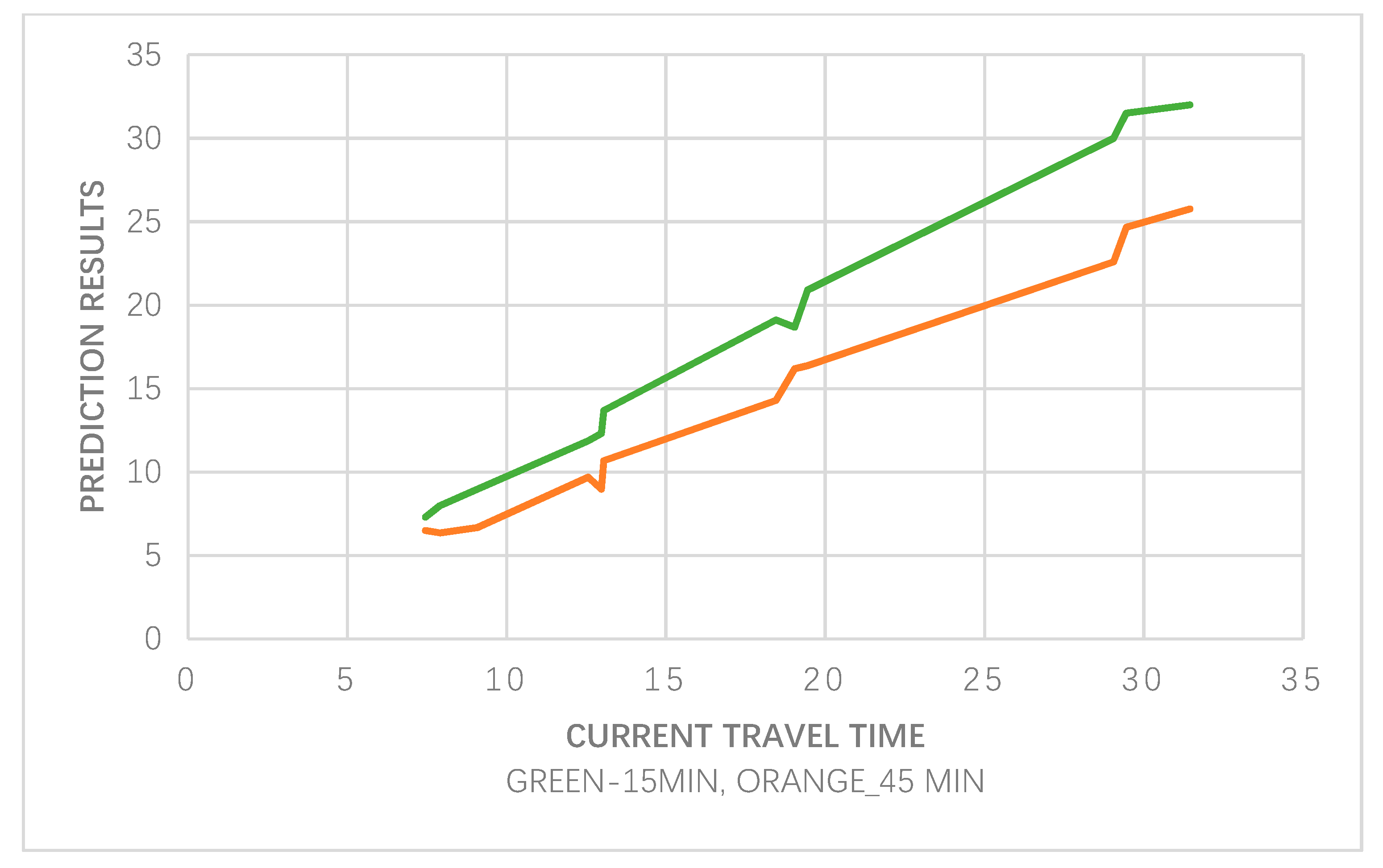
Since the most important relative feature is the same for different prediction horizons, the partial dependence function graphs between predicted travel time and actual travel time in the current period are shown in Figure 8. It can be found that current travel time has a highly linear relationship with the predicted travel time; however, the curve behaves differently for different prediction horizons. Furthermore, when the prediction horizon increases (from 15 to 45 min), the change rate of the curve gradually decreases, which demonstrates that travel time in the current period has less impact on the TTP. It indicates that the model’s predicted performance decreases as the prediction horizon increases.

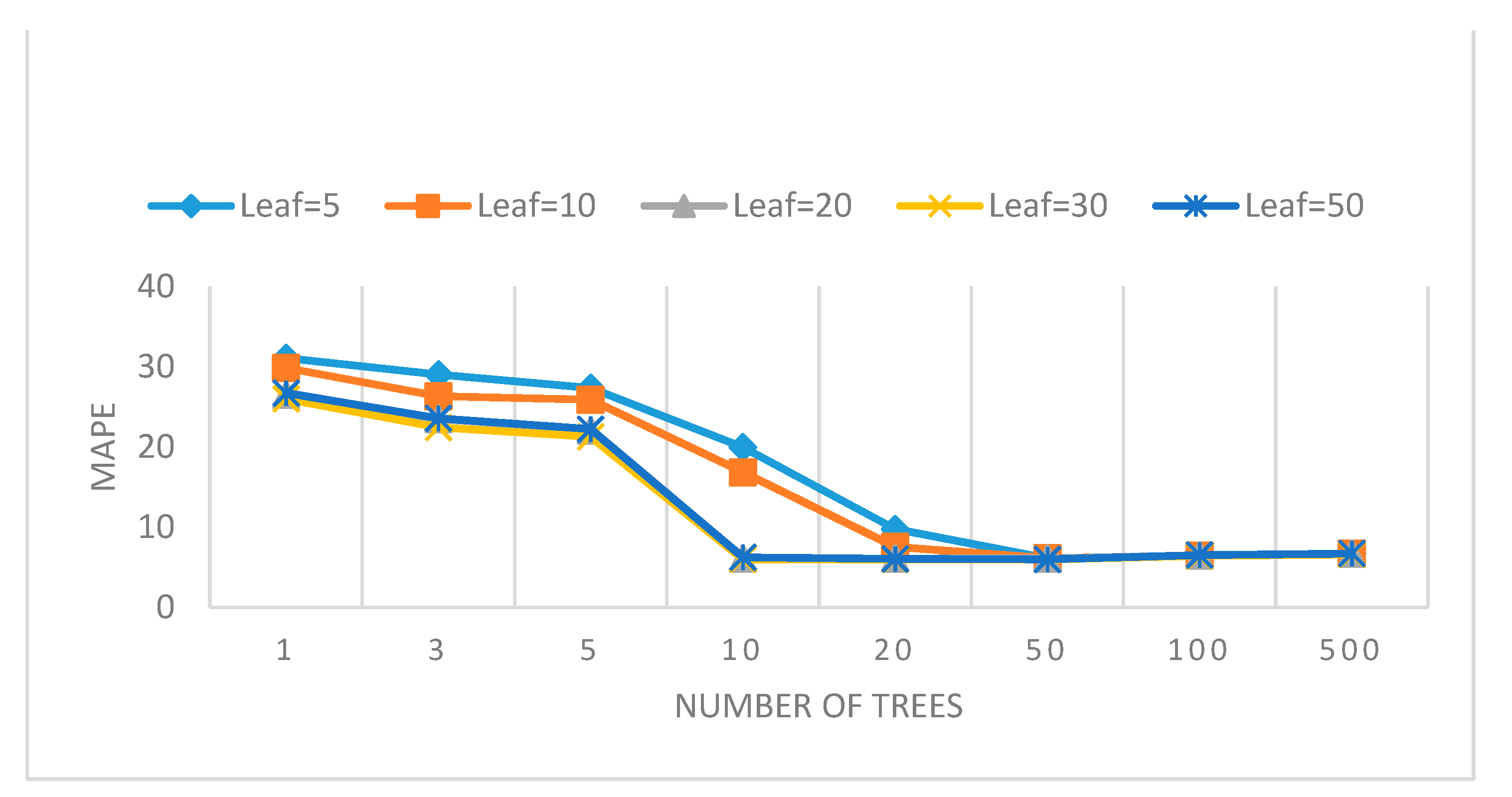
In machine learning, overfitting typically occurs when the model corresponds perfectly to the sample set of data, and therefore, the model may fail to fit additional data or predict future observations reliably. RF is an ensemble of DTs. The single DT is sensitive to data variations, which can overfit to noise in the data. While in the RF model, as the number of trees increases, the tendency of overfitting decreases. Among the four applied algorithms, due to the bagging and random feature selection process, the RF was deemed as not prone to overfitting and very noise-resistant. However, it can still be improved, and in order to avoid overfitting in RF, the hyper-parameters of the algorithm should be tuned very carefully.

5. Conclusions and Recommendations

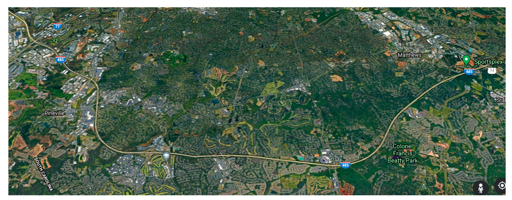
Short-term TTP can be an important planning tool for both individual and public transportation. In general, the benefits of TTP come from three aspects [6]: Saving travel time and improving reliability for the travelers; improving the reliability of delivery and the service quality and cutting costs for logistics [40]. TTP is the key to traffic system management. Machine learning algorithms base on large data are generally more capable of searching and aggregating previously undetectable patterns and nonlinearity, and therefore possess the power to predict more accurate results. In both cases, it is expected that the application of accurate TTP can greatly help improve the level of service and enhance travel planning by reducing errors between the actual and predicted travel time. In this study, four non-parametric state-of-the-art machine learning methods, i.e., DT, XGBoost, RF, and LSTM (three from ensemble tree-based learning, and one from neural network), were developed and compared. After the data processing and feature selection process, all four methods were estimated, and the best combination of model parameters inherent in each model was also identified and used. In the model training and validation process, the sample dataset from selected road segments in I-485 Charlotte are used. Experimental results indicated that the RF is the most promising approach among all the methods that were developed and tested. The results also showed that all ensemble learning methods (i.e., RF and XGBoost) achieved high estimation accuracy and significantly outperformed the other methods. Furthermore, the ensemble learning methods run efficiently on large data sets due to the reduced model complexity of tree-based methods. Moreover, from a statistical point of view, these methods can overcome overfitting to some extent. It is well known that overfitting means that the estimated model fits the training data too well, which is typically caused by the model function being too complicated to consider each data point and even outliers.

However, this study still has some limitations. First, the TTP models were developed under normal traffic conditions and do not consider unexpected conditions (e.g., special events such as accidents and work zone activities). In addition, the data collected from the selected freeway segments were limited in diversity. There is the hope that with the development and popularization of real-time collection and uploading of traffic data acquisition technology (such as GPS trajectories, smartphones), sufficient data will provide the possibility for developing a more accurate TTP model. Furthermore, to identify whether the TTP is region-specific, further research is needed to replicate this study in other road categories using other types of data sources. Further results need to be achieved to compare all methods to further demonstrate whether the ensemble tree-based learning methods have better predictive accuracy in short-term TTP. Moreover, variables such as the characteristics of drivers and the impact of sun glare and other environmental hazards that could increase congestion will need to be incorporated into the model. Some experimental results have shown that the combination methods have a better prediction result than using one method alone [41,42,43]. Even though the combination models have proven to be superior in terms of prediction accuracy and stability, they should be carefully considered in future research.

References

1. Chien, S.I.-J.; Kuchipudi, C.M. Dynamic Travel Time Prediction with Real-Time and Historic Data. J. Transp. Eng. 2003, 129, 608–616. [Google Scholar] [CrossRef]
2. Oh, S.; Byon, Y.-J.; Jang, K.; Yeo, H. Short-term Travel-time Prediction on Highway: A Review of the Data-driven Approach. Transp. Rev. 2015, 35, 4–32. [Google Scholar] [CrossRef]
3. Van Lint, J.W.C. Reliable Travel Time Prediction for Freeways; TRAIL Research School: Delft, The Netherlands, 2004. [Google Scholar]
4. Chou, C.-H.; Huang, Y.; Huang, C.-Y.; Tseng, V.S. Long-Term Traffic Time Prediction Using Deep Learning with Integration of Weather Effect; Springer: Cham, Switzerland, 2019; pp. 123–135. [Google Scholar]
5. Shen, L. Freeway Travel Time Estimation and Prediction Using Dynamic Neural Networks. Ph.D. Thesis, Florida International University, Miami, FL, USA, 2008. [Google Scholar]
6. Abdollahi, M.; Khaleghi, T.; Yang, K. An integrated feature learning approach using deep learning for travel time prediction. Expert Syst. Appl. 2020, 139, 112864. [Google Scholar] [CrossRef]
7. Dharia, A.; Adeli, H. Neural network model for rapid forecasting of freeway link travel time. Eng. Appl. Artif. Intell. 2003, 16, 607–613. [Google Scholar] [CrossRef]
8. Park, D.; Rilett, L.R. Forecasting Freeway Link Travel Times with a Multilayer Feedforward Neural Network. Comput. Civ. Infrastruct. Eng. 1999, 14, 357–367. [Google Scholar] [CrossRef]
9. Yildirimoglu, M.; Geroliminis, N. Experienced travel time prediction for congested freeways. Transp. Res. Part B Methodol. 2013, 53, 45–63. [Google Scholar] [CrossRef] [Green Version]
10. Zhang, Y.; Haghani, A. A gradient boosting method to improve travel time prediction. Transp. Res. Part C Emerg. Technol. 2015, 58, 308–324. [Google Scholar] [CrossRef]
11. Vapnik, V.N. The Nature of Statistical Learning Theory; Springer: New York, NY, USA, 1995. [Google Scholar]
12. Wu, C.-H.; Ho, J.-M.; Lee, D. Travel-Time Prediction with Support Vector Regression. IEEE Trans. Intell. Transp. Syst. 2004, 5, 276–281. [Google Scholar] [CrossRef] [Green Version]
13. Bin, Y.; Zhongzhen, Y.; Baozhen, Y. Bus Arrival Time Prediction Using Support Vector Machines. J. Intell. Transp. Syst. 2006, 10, 151–158. [Google Scholar] [CrossRef]
14. Xumei, C.; Huibo, G.; Wang, J. BRT vehicle travel time prediction based on SVM and Kalman filter. J. Transp. Syst. Eng. Inf. Technol. 2012, 12, 29–34. [Google Scholar]
15. Rupnik, J.; Davies, J.; Fortuna, B.; Duke, A.; Clarke, S.S.; Jan, R.; John, D.; Bla, F.; Alistair, D.; Stincic, C.S. Travel time prediction on highways. In Proceedings of the 2015 IEEE International Conference on Computer and Information Technology, Liverpool, UK, 26–28 October 2015; pp. 1435–1442. [Google Scholar]
16. Li, Y.; Fujimoto, R.M.; Hunter, M.P. Online travel time prediction based on boosting. In Proceedings of the 2009 12th International IEEE Conference on Intelligent Transportation Systems, St. Louis, MO, USA, 4–7 October 2009; pp. 1–6. [Google Scholar]
17. Mendes-Moreira, J.; Jorge, A.M.; De Sousa, J.F.; Soares, C. Improving the accuracy of long-term travel time prediction using heterogeneous ensembles. Neurocomputing 2015, 150, 428–439. [Google Scholar] [CrossRef]
18. Zhang, W.; He, R.; Xiao, Q.; Ma, C. Taxi carpooling model and carpooling effects simulation. Int. J. Simul. Process Model. 2017, 12, 338–346. [Google Scholar] [CrossRef]
19. Jammalamadaka, S.R.; Qiu, J.; Ning, N. Predicting a stock portfolio with the multivariate bayesian structural time series model: Do news or emotions matter? Int. J. Artif. Intell. 2019, 17, 81–104. [Google Scholar]
20. Precup, R.-E.; Teban, T.-A.; Albu, A.; Borlea, A.-B.; Zamfirache, I.A.; Petriu, E.M. Evolving Fuzzy Models for Prosthetic Hand Myoelectric-Based Control. IEEE Trans. Instrum. Meas. 2020, 69, 4625–4636. [Google Scholar] [CrossRef]
21. Wang, Z.; Fu, K.; Ye, J. Learning to estimate the travel time. In Proceedings of the 24th ACM SIGKDD International Conference on Knowledge Discovery & Data Mining, London, UK, 19 July 2018; pp. 858–866. [Google Scholar]
22. Sharmila, R.B.; Velaga, N.R.; Kumar, A. SVM-based hybrid approach for corridor-level travel-time estimation. IET Intell. Transp. Syst. 2019, 13, 1429–1439. [Google Scholar] [CrossRef]
23. Lee, E.H.; Kho, S.-Y.; Kim, D.-K.; Cho, S.-H. Travel time prediction using gated recurrent unit and spatio-temporal algorithm. Proc. Inst. Civ. Eng. Munic. Eng. 2021, 174, 88–96. [Google Scholar] [CrossRef]
24. Wang, Z.J.; Li, D.B.; Cui, X. Travel time prediction based on LSTM neural network in precipitation. J. Transp. Syst. Eng. Inf. Technol. 2020, 20, 137–144. [Google Scholar]
25. Zhao, L.; Chien, S.I.-J. Analysis of Weather Impact on Travel Speed and Travel Time Reliability. In Proceedings of the 12th COTA International Conference of Transportation Professionals, Beijing, China, 3–6 August 2012; pp. 1145–1155. [Google Scholar] [CrossRef]
26. Koetse, M.J.; Rietveld, P. Climate change, adverse weather conditions, and transport: A literature survey. In Proceedings of the 9th Network on European Communication and Transportation Activities Research (NECTAR) Conference, Porto, Portugal, 9 September 2007. [Google Scholar]
27. Kuncheva, L.I.; Whitaker, C.J. Measures of Diversity in Classifier Ensembles and Their Relationship with the Ensemble Accuracy. Mach. Learn. 2003, 51, 181–207. [Google Scholar] [CrossRef]
28. Polikar, R. Ensemble Learning. In Ensemble Machine Learning; Springer: Boston, MA, USA, 2012; pp. 1–34. [Google Scholar]
29. Greenhalgh, J.; Mirmehdi, M. Real-Time Detection and Recognition of Road Traffic Signs. IEEE Trans. Intell. Transp. Syst. 2012, 13, 1498–1506. [Google Scholar] [CrossRef]
30. Chen, T.; Guestrin, C. Xgboost: A scalable tree boosting system. In Proceedings of the 22nd ACM SIGKDD International Conference on Knowledge Discovery and Data Mining, San Francisco, CA, USA, 13–17 August 2016; pp. 785–794. [Google Scholar]
31. Kankanamge, K.D.; Witharanage, Y.R.; Withanage, C.S.; Hansini, M.; Lakmal, D.; Thayasivam, U. Taxi trip travel time prediction with isolated XGBoost regression. In Proceedings of the 2019 Moratuwa Engineering Research Conference (MERCon), Moratuwa, Sri Lanka, 3–5 July 2019; pp. 54–59. [Google Scholar]
32. Kearns, M. Thoughts on hypothesis boosting. Mach. Learn. Class Proj. 1988, 45, 105, Unpublished manuscript. [Google Scholar]
33. Fan, W.; Chen, Z. Predicting Travel Time on Freeway Corridors: Machine Learning Approach; No. 2019 Project 01; Center for Advanced Multimodal Mobility Solutions and Education: Charlotte, NC, USA, 2020. [Google Scholar]
34. Schmidhuber, J.; Wierstra, D.; Gagliolo, M.; Gomez, F. Training recurrent networks by evolino. Neural Comput. 2007, 19, 757–779. [Google Scholar] [CrossRef] [Green Version]
35. Wang, D.; Zhang, J.; Cao, W.; Li, J.; Zheng, Y. When will you arrive? Estimating travel time based on deep neural networks. In Proceedings of the AAAI Conference on Artificial Intelligence, New Orleans, LA, USA, 26 April 2018; Volume 32. [Google Scholar]
36. Cheng, J.; Li, G.; Chen, X. Research on Travel Time Prediction Model of Freeway Based on Gradient Boosting Decision Tree. IEEE Access 2018, 7, 7466–7480. [Google Scholar] [CrossRef]
37. Breiman, L. Random forests. Mach. Learn. 2001, 45, 5–32. [Google Scholar] [CrossRef] [Green Version]
38. Du, L.; Peeta, S.; Kim, Y.H. An adaptive information fusion model to predict the short-term link travel time distribution in dynamic traffic networks. Transp. Res. Part B Methodol. 2012, 46, 235–252. [Google Scholar] [CrossRef]
39. Fu, K.; Meng, F.; Ye, J.; Wang, Z. CompactETA: A fast inference system for travel time prediction. In Proceedings of the 26th ACM SIGKDD International Conference on Knowledge Discovery & Data Mining, Virtual Event, CA, USA, 23 August 2020; pp. 3337–3345. [Google Scholar]
40. Abdollahi, M.; Arvan, M.; Omidvar, A.; Ameri, F. A simulation optimization approach to apply value at risk analysis on the inventory routing problem with backlogged demand. Int. J. Ind. Eng. Comput. 2014, 5, 603–620. [Google Scholar] [CrossRef]
41. Zou, N.; Wang, J.; Chang, G.L. A reliable hybrid prediction model for real-time travel time prediction with widely spaced detectors. In Proceedings of the 2008 11th International IEEE Conference on Intelligent Transportation Systems, Beijing, China, 12–15 October 2008; pp. 91–96. [Google Scholar]
42. Mendes-Moreira, J.; Jorge, A.M.; de Sousa, J.F.; Soares, C. Comparing state-of-the-art regression methods for long term travel time prediction. Intell. Data Anal. 2012, 16, 427–449. [Google Scholar] [CrossRef] [Green Version]
43. Huang, H.; Pouls, M.; Meyer, A.; Pauly, M. Travel Time Prediction Using Tree-Based Ensembles. In Proceedings of the International Conference on Computational Logistics, Enschede, The Netherlands, 28–30 September 2021; Springer: Cham, Switzerland, 2020; pp. 412–427. [Google Scholar]
Figure 1. Taxonomy of TTP.
Sustainability 13 07454 g001
Figure 2. Aerial photograph of the study site.
Sustainability 13 07454 g002
Figure 3. RF algorithm flow chart.
Sustainability 13 07454 g003
Figure 4. Memory unit of LSTM.
Sustainability 13 07454 g004
Figure 5. RF travel time prediction model performance.
Sustainability 13 07454 g005
Figure 6. Selected observation segments in case study.
Sustainability 13 07454 g006
Figure 7. MAPE of different observation points with a different prediction time range.
Sustainability 13 07454 g007
Figure 8. Partial dependence function graph for different prediction horizon. Green, 15 min prediction horizon; orange, 45 min prediction horizon.
Sustainability 13 07454 g008