Abstract
Achieving the seventeen United Nations Sustainable Development Goals (SDGs) requires accurate, consistent, and accessible population data. Yet many low- and middle-income countries lack reliable or recent census data at the sufficiently fine spatial scales needed to monitor SDG progress. While the increasing abundance of Earth observation-derived gridded population products provides analysis-ready population estimates, end users lack clear use criteria to track SDGs indicators. In fact, recent comparisons of gridded population products identify wide variation across gridded population products. Here we present three case studies to illuminate how gridded population datasets compare in measuring and monitoring SDGs to advance the “fitness for use” guidance. Our focus is on SDG 11.5, which aims to reduce the number of people impacted by disasters. We use five gridded population datasets to measure and map hazard exposure for three case studies: the 2015 earthquake in Nepal; Cyclone Idai in Mozambique, Malawi, and Zimbabwe (MMZ) in 2019; and flash flood susceptibility in Ecuador. First, we map and quantify geographic patterns of agreement/disagreement across gridded population products for Nepal, MMZ, and Ecuador, including delineating urban and rural populations estimates. Second, we quantify the populations exposed to each hazard. Across hazards and geographic contexts, there were marked differences in population estimates across the gridded population datasets. As such, it is key that researchers, practitioners, and end users utilize multiple gridded population datasets—an ensemble approach—to capture uncertainty and/or provide range estimates when using gridded population products to track SDG indicators. To this end, we made available code and globally comprehensive datasets that allows for the intercomparison of gridded population products.
1. Introduction
The United Nations Sustainable Development Goals (SDGs) aim to end global poverty by 2030 and ensure a sustainable future [1]. To accomplish this, the SDGs outline a set of seventeen interlinked and shared objectives to improve economic and health outcomes in low- and middle-income countries (LMICs) while simultaneously reducing environmental degradation and tackling climate change for all countries [2,3]. The SDGs were designed to overcome the measurement challenges of the Millennium Development Goals [4] by outlining a clear set of indicators to track progress. Accordingly, global partnerships—such as the Sustainable Development Solutions Network [5] and the Global Partnership for Sustainable Development Data [6]—were established to provide countries with best practices to monitor SDG indicators and to support decision making to achieve the SDGs [7]. These partnerships increasingly advocate for countries to leverage the considerable amount of Earth observations (EO) data to track SDG indicators. In particular, analysis-ready EO data present a systematic, affordable, and longitudinal pathway to track SDG indicators that are specifically tractable for decision makers [8,9,10,11,12]. However, researchers, practitioners, and decision makers collectively lack guidance on how to best utilize wide-ranging and context-specific EO data to monitor SDG indicators.
This lack of guidance creates challenges for the SDGs’ “leave no one behind” agenda. Not only does tracking many SDG indicators require accurate and accessible information on where people live, but achieving the SDGs entails providing services to people. Indeed, 73 SDG indicators require population data to track them [5]. Yet, due to the lack of reliable and consistent census data for many countries [13,14,15], we do not have information regarding where people live at sufficiently fine spatial scales to measure, monitor, and map changes in the distribution of populations relevant to many of the SDGs [13]. As such, EO-derived gridded population products present a vital source of population information to track the SDGs that continue to gain attention [5,16,17,18,19]. Each gridded population product offers spatially explicit representations of population distributions in a comparable, consistent manner that can be well suited to monitor SDG indicators across disparate geographies and time points. We chose to focus on gridded population data for two reasons. First, the gridded population products are receiving increasing use by a wide range of researchers, practitioners, and decision makers. Second, the methodologies and EO input data used to develop gridded population products continue to advance rapidly.
Given the wide range of gridded population products available, new “fitness for use” guidelines outline the tradeoffs and benefits the various gridded products offer for monitoring many SDG indicators [5,20]. However, the findings from recent studies [21,22,23,24,25] that have compared how gridded populations products allocate population illuminate the need for comparison of these datasets in the context of measuring and monitoring the SDGs. For example, a recent comparison of gridded population products against government-derived gridded census data in Sweden found wide variation in the accuracy of gridded population datasets to measure pixel-level population estimates [21]. Similarly, another recent study identified wide disagreement in both the location of and population estimates for urban settlements in Africa across gridded population products [25].
Broadly, the variation across products is explained by three reasons (for a recent review, see [20]). First, each gridded population product relies on different types of EO-based ancillary input data and production methods. Second, gridded population products differ in spatial resolution, projections, and temporal coverage. Third, for all but one product (Table 1), the process of creating the gridded distribution of population involves a disaggregation of census or administrative unit area counts into individual cells by relying on various EO-based (e.g., land cover type, settlement presence, nighttime light intensity) and geospatial covariates (e.g., buildings, roads, elevation) that vary in characteristics, quality, and accuracy [20]. Simply put, each gridded population product will likely tell a different story. In countries where reliable or recent fine-resolution census data are not available—precisely the context in which EO-enhanced gridded population datasets were designed to be employed—few independent fine-resolution micro censuses exist against which to assess the accuracy of gridded population products. Furthermore, aside from World Population Estimate 2016 (WPE-16), all current global gridded population products lack uncertainty estimates [5,20]. Until robust validation studies are available or uncertain estimates are produced, there remains a need to assess how different population data sets may influence the methods and results employed to monitor and evaluate progress towards SDGs.

Table 1.
Summary of near-global coverage gridded population datasets included in this study. For further information, see [20] and the PopGrid Data Collaborative [35].
Here we present three case studies to illuminate how gridded population datasets compare in measuring and monitoring SDGs and to advance the “fitness for use” guidance. Our focus is on SDG Target 11.5:
“By 2030, significantly reduce the number of deaths and the number of people affected and substantially decrease the direct economic losses relative to global gross domestic product caused by disasters, including water-related disasters, with a focus on protecting the poor and people in vulnerable situations.”
In the context of SDG Target 11.5, we compare how five gridded population data products (Table 1) measure the population exposed to the 2015 earthquake in Nepal and Cyclone Idai in Mozambique, Malawi, and Zimbabwe (henceforth referred as MMZ) in 2019, as well as populations susceptible to flash floods in Ecuador. By focusing on a range of geographic and country-specific contexts across several hazards, our results provide insights into the ways in which the construction of different gridded population products across geographies affects the resulting calculation of the potentially affected populations.
Furthermore, we explore how gridded population products can be applied to other global frameworks, such as towards the Sendai Framework for Disaster Risk Reduction Targets [26]. Specifically, to achieve the first four targets (a–d), disaster risk monitoring requires accurate estimates of impacts on people and/or property [27]. Our work contributes to the Sendai Framework Global Target B: “Substantially reduce the number of affected people globally by 2030, aiming to lower the average global figure per 100,000 between 2020–2030 compared with 2005–2015.” Beyond the importance of gridded data for calculating these indicators, however, we note that accurate population estimates are also vital to emergency management and humanitarian agencies in the post-disaster response phase, when assessments of the number of people affected directly translates to supplies and disaster finance being prioritized (or deprioritized) across spatial units of interest [28]. Thus, the work presented here contributes to an understanding of the potential for operational uses of various gridded population products.
We chose five gridded populations products (Table 1) due to their availability at the time of analysis and their global coverage. Our analysis focuses on the comparison of these different gridded products and why estimates are similar or dissimilar in different socio-economic and hazard contexts. Given the lack of “ground truth” micro census population estimates for the regions compared, we do not assess the accuracy of the gridded population products themselves. However, the analysis provided does inform end users of the potential pros and cons of using these datasets in the context of measuring SDG 11.5.
We have two interrelated objectives. First, we map and quantify geographic patterns of agreement/disagreement across gridded population products for Nepal, MMZ, and Ecuador, including delineating urban from rural populations estimates. Several methodologies have been used to compare products [21,22,23,24,25]. For the initial step, we identify the number of rasters that agree if a given pixel is inhabited or not. Next, we assess pixel-level variation across the five gridded population products by plotting the minimum pixel values against pixel ranges to identify outliers and showcase the contrast in pixel-level measurements. Then, for each gridded product, we examine transects through the primary urban centers impacted by the hazards to both visually and quantitatively demonstrate the variability in population estimates by product across the urban-rural continuum [29].
The second objective aims to situate our first objective within the context of measuring, monitoring, and mapping SDG 11.5. For each dataset, we estimate the total number of people, stratified by urban and rural populations, exposed to each hazard. For Nepal, we compare estimates across seismic intensity levels during the 2015 Earthquake. With Cyclone Idai, we compare estimates of population inundated by water detected by Sentinel-1 EO platform and exposed to wind speed zones. Lastly, in Ecuador, we quantify and map populations living in zones across levels of susceptibility to flash floods. We emphasize that our results do not quantify error or validate population estimates across gridded population products. We note that the urban land cover designation we employ (Section 2.1) is for comparative purposes only. Our analysis does not assess how gridded population products measure urban populations and urban boundaries (for further detail see [25,29]). All our code and data used in this analysis is open source and freely available for other scholars and practitioners to develop their own use cases. This includes global raster datasets that allow for the intercomparison of gridded population products.
2. Materials and Methods
2.1. Dataset Descriptions
2.1.1. Population Data
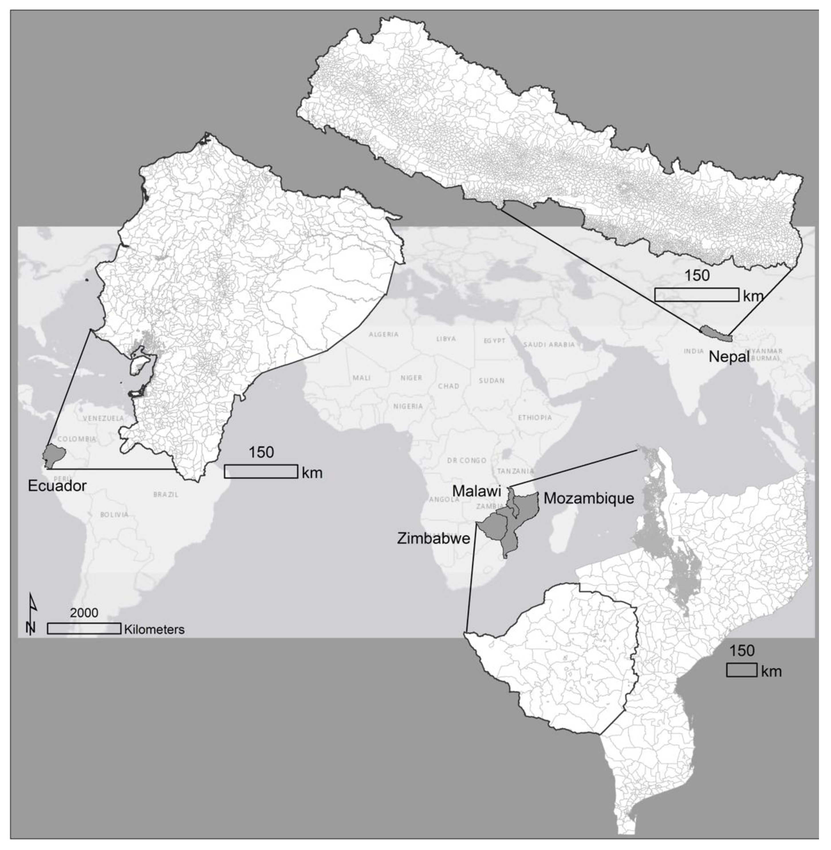
We focus on three geographies of interest—Nepal, the region of Mozambique, Malawi, and Zimbabwe (MMZ), and Ecuador (Figure 1)—to explore how the gridded population products measure populations related to SDG 11.5 across a range of geographic contexts. Nepal, a relatively small country, is landlocked between China’s Tibet Autonomous Region and India, and is very mountainous. As hazards do not respect political boundaries, we present MMZ to measure exposure in a cross-border use case. Indeed, population exposure to Cyclone Idai spanned from Mozambique’s low-elevation coastal zones, to Malawian settlements near Lake Malawi, to the relatively high-elevation settlements in Zimbabwe. Ecuador presents both a mountainous and a coastal geography to examine hazards, as well as higher levels of economic development compared to the other two geographies of interest. We intentionally chose countries and study areas that coincided with hazard events that matched the gridded population product dates and span LMIC contexts.

Figure 1.
Map of three geographies of interest with administrative input units for GWP-15 overlaid.
The five gridded population products we use are (Table 1): World Population Estimates 2016 [30]; the Global Human Settlement Layer Population 2015 (GHS-15) [31]; Gridded Population of the World version 4 2015 (GPW-15) [32]; LandScan 2015 (LS-15) [33]; and WorldPop 2016 (WP-16) [34]. For a complete description of how each gridded population product is produced, see [20,25], as well as the PopGrid Data Collaborative [35].
Aside from GPW-15, the gridded population datasets used in this study rely on relationships between EO data and human settlement patterns to disaggregate the finest available administrative unit level population data into pixels (Table 1). A higher administrative level corresponds to a finer resolution administrative unit. Additionally, only LS-15 focuses on daytime, or ambient population, whereas the other products aim to capture nighttime residential population [35]. Last, aside from GHS-15, which disaggregates administrative unit-level population only within pixels identified as containing built settlements (constrained), all other products disaggregate administrative unit-level population over all land pixels globally (unconstrained). All products we use are at 1 km spatial resolution. We use GPW-15 as a baseline for comparison, as it is the underlying population data for both GHS-15 and WP-16. Finally, we include United Nations population estimates for each geography of interest for 2015 (Table 2) [36].
Table 2.
Allocation of population and pixel-level agreement across five gridded population products for Nepal, MMZ, and Ecuador circa 2015. For each geography of interest the number and level of input administrative units is listed. Note urban, rural, and total populations are in millions.
2.1.2. Hazards Impacts & Data
2015 Nepal Earthquake
On 25 April 2015, a 7.8-magnitude earthquake struck approximately 80 km northwest of Kathmandu, the country’s capital, at 6:11 UCT [39]. Official estimates state that the earthquake killed more than 8000 people, injured 21,000 more people, and displaced at least 2 million people in total [40]. Some 600,000 homes were destroyed, with another quarter million damaged [41]. The government estimated that reconstruction costs would surpass $7 billion, or a third of Nepal’s GDP in the prior fiscal year [42]. Data and information on the earthquake was obtained from the US Geological Survey (USGS) [39]. USGS ShakeMap shapefiles were used to estimate earthquake impacts by “Instrumental Intensity”, which is a proxy for Modified Mercalli Intensity (a qualitative index that can not strictly be determined by instruments).
2019 Cyclone Idai
Cyclone Idai made landfall near Beira, Mozambique, on 14 March 2019. The storm had sustained wind >120 km/h. By March 16, the storm had tracked across Southern Mozambique into Zimbabwe. Flooding was observed throughout Malawi, Mozambique, and Zimbabwe, directly impacting 1.85 million people across MMZ [43]. The immediate financial requirement of the response was estimated to be nearly $300 million [43].
To measure maximum flood extent, we use a 90 m raster available from the World Food Program that captures maximum flood extent as of 21 March 2019 [44]. The raster is derived from Sentinel-1 data obtained from 12 to 21 March 2019 and ARC Flood Extent Depiction Model (AFED) detecting non-persistent water (7–16 March and 20 March 2019). We resampled the 90 m flood raster to 1 km and reprojected it to match GPW-15. Data on wind speeds were downloaded from the Global Disaster Alert and Coordination System [45], with shapefiles delineating zones impacted by 60, 90, 120 km/h wind speed thresholds.
Ecuador Flash Flood Susceptibility
In Ecuador, as well as on a global scale, flash floods are one of the most deadly types of flood with distinct spatiotemporal physical and impact-related characteristics [46,47,48,49]. Early warning systems exist for floods in many countries; however, they are rarely linked to resilience programming that can decrease risk of a flash flood disaster. While a long time series of impact data for flash floods (and any type of floods) does not openly exist in Ecuador [50], financial estimates of flood impact in the country can be acquired in some instances, with a reported US$238 million in flood impact in 2012 [51].
To represent the susceptibility for flash flooding at the catchment scale in Ecuador, a new vector dataset is derived from geophysical and non-geophysical data [52]. The susceptibility layer was built using a principal component analysis (PCA) derived weighted mean [53] of geographic indicators known to drive the flash flood potential of a catchment, related to geomorphology, drainage systems, and surface characteristics [54,55,56]. Geographic indicators such as slope, curvature, stream order, area of contributing sources, density of drainage, land cover, and sand content [57,58,59,60] were attributed to each catchment, using the predefined level 12 watershed units of HydroSHEDS [61], developed by the Conservation Science Program of World Wildlife Fund (WWF). The resulting flash flood susceptibility composite layer is normalized and reclassified into an equal count discrete flash flood susceptibility index from 1 to 10, low to high susceptibility, respectively, and represents the relative ranking of Ecuador catchments according to their increased susceptibility to generate flash flooding in the case of heavy rain.
Urban/Rural Data
To identify urban versus rural population estimates across the five gridded population products, we use an urban-rural binary land cover classification derived from MODIS data—the MODIS global urban extent product (MGUP) [62]. This dataset is available from 2002 to 2018 at 500 m spatial resolution. We resample the 2015 MGUP data to 1 km and projected it to match GPW-15. We employ MGUP as a relatively independent estimation of where urban settlements exist, as other MODIS products are an input in three of the five gridded population products (Table 1). In addition, we recognize that MGUP is one among many datasets that delineate urban from rural land cover globally and that binary urban/rural categorizations have well-known limitations [29]. As such, the MGUP urban/rural designation we employ is, to a degree, arbitrarily defined with an intent more on trying to better understand underlying population distribution methods, not a statement on what population is urban and what is rural.
2.2. Raster Processing & Analysis
The five global gridded population rasters and the MGUP urban/rural land cover raster were spatially co-registered (see Supplemental Information for the detail) and clipped using the GADM level 0 administrative units for Nepal, MMZ, and Ecuador (excluding islands). Across all five gridded population datasets, for the three study areas we map uninhabited pixels, calculate maximum and minimum population (as well as the range (maximum–minimum) at the pixel level), and measure urban and rural population estimates according to the MGUP urban/rural classification (Table 2). To identify outliers and highlight the variation in pixel-level estimates, we plotted pairwise pixel minimum population estimates against pixel ranges (Figure 2). We then examine 7 km by 61 km transects through three urban areas—Katmandu for Nepal, Beira for MMZ, and Quito for Ecuador—to visually and quantitatively demonstrate how the products’ population estimates compare at the pixel level across the urban-rural continuum.
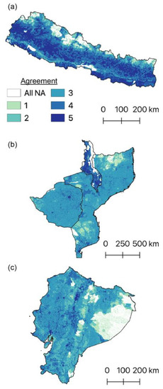
Figure 2.
Spatial agreement of if a pixel is inhabited for five gridded population datasets for (a) Nepal, (b) MMZ, and (c) Ecuador. Values correspond to the number of rasters in agreement that a pixel is inhabited. White shows that all five gridded population datasets agree that a pixel is uninhabited. The higher agreement for Nepal (a) and Malawi (b) is a result of the higher number of administrative input units. Note that the spatial scale of each panel is different.
To compare estimates of populations impacted by the three hazards under study, we sum the populations by hazard criteria for the five gridded population products, separating urban and rural estimates. For the 2015 Earthquake in Nepal, we sum the population exposed by the USGS Shakemap “Instrumental Intensity” contour polygons. For Cyclone Idai, we sum the population exposed by wind speed buffer and flooded area. Finally, for the flash flood in Ecuador we sum the population exposed by the susceptibility index layer.
3. Results
3.1. Pixel-Level Comparisons
Four broad patterns emerged when comparing how the five gridded population datasets allocate populations in Nepal, MMZ, and Ecuador. First, we found widespread pixel-level variation in agreement across gridded population products of whether or not a given pixel is inhabited. Broadly, GHS-15 and WPE-16 identify a smaller proportion of inhabited pixels regardless of geography. We found that Nepal had the highest proportion of agreement, with all five gridded population products agreeing that 76% of pixels are either inhabited or uninhabited (Figure 2a). Only 67% for MMZ (Figure 2b) and 62% for Ecuador (Figure 2c) had full agreement by all five products. WP-16, LS-15, and GPW-15 tended to distribute population to a far greater number of pixels, unlike GHS-15 and WPE-16 (Table 2). For example, for MMZ, 85% of pixels in WPE-16 and 89% of pixels in GHS-15 were uninhabited. In contrast, WP-16, LS-15, and GPW-15 identified that only 11%, 14%, and 8% of pixels in MMZ are uninhabited, respectively.
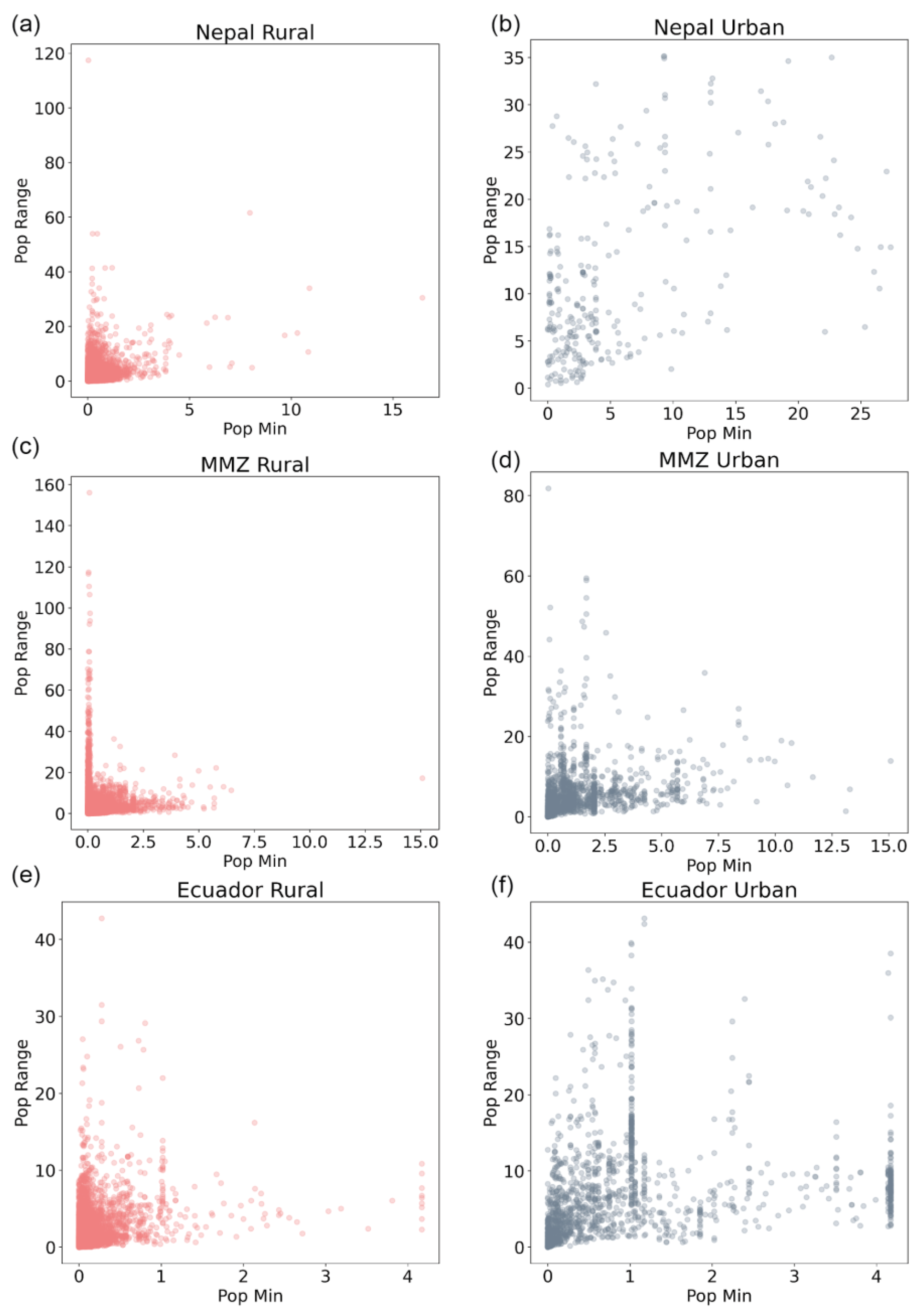
Second, we documented extreme pixel-level population estimation disparities across gridded population products (Figure 3) and identified outliers. In pairwise comparison between the minimum pixel values with the range identified across all five gridded population products, for Nepal and MMZ, 27 rural pixels with minimums of 0–1000 people had ranges that exceed 50,000 people. Rural outliers in Ecuador do not have the same magnitude as Nepal or MMZ. Yet we still identified 8 rural pixels with minimum values of 0–1000 that have a range that exceeds 25,000 people in Ecuador. In the most extreme example, one pixel on the border of Nepal and India was estimated by GHS-15 to have nearly 120,000 residents (Figure 3a, Table 2). GPW-15 and WP-16 allocate 2392 and 730 people, respectively, to the same pixel, and the other two products identify fewer than 125 people. A visual inspection of high-resolution WorldView imagery from Google Earth reveals that the pixel mostly corresponds to a river with sand bars. For context, recently the United Nations Statistical Commission released standards identifying pixels within urban cores as having a population density of at least >1500 people per km2 [63].
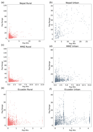
Figure 3.
To identify outliers and pixel-level variation across gridded population products, the minimum population estimates (thousands) for each pixel are plotted against the population range (thousands), separated by rural and urban pixels, for Nepal (a,b), MMZ (c,d), and Ecuador (e,f). An example of an outlier is evident in panel (a) with one rural pixel having a range of more than 120,000 people.
Third, we found a clear pattern that WPE-16 total population estimates greatly exceeded the other four datasets. For instance, in MMZ, we found that WPE-16 exceeds the total population measured by the other gridded population datasets by 6–11 million people (Table 2), and exceeds UN population estimates for all three geographies of interest as well. As another example, while GHS-15 tended to prioritize allocating population to urban settlements compared to the other gridded population datasets, WPE-16 identified more urban residents in Nepal, by as much as 500,000 people, than the other four gridded population products.
Fourth, GHS-15 allocated a greater share of the total population to urban areas (as defined by the MGUP dataset) than the other four products for all three regions under study. For example, in Ecuador, GHS-15 estimated that 51% of the total population is urban. LS-15 was ranked second for Ecuador, allocating 47.9% of the total population to urban areas, followed by WPE-16 with 43.67% of the total population estimated as urban. In MMZ, GHS-15 again led in terms of the share of total population allocated to urban areas, again followed by LS-15. In Nepal, WP-16 and GPW-15, respectively, followed GHS-15 in terms of the share of total populations allocated to urban areas. Nonetheless, all five gridded population products underestimated the total urban population for all three geographies of interest when compared to 2018 United Nations World Urbanization Prospect estimates [36]. Indeed, even GHS-15 estimated nearly 50% fewer urban residents in MMZ than official UN counts.
Because the MGUP rural-urban binary designation does not capture how population density varies across that rural-urban continuum [29], Figure 4 illustrates how each gridded population product allocates population moving away from major urban centers. For the Kathmandu transect (Figure 4a), there is far closer agreement in populations among the products compared to Beira (Figure 4b) and Quito (Figure 4c). GPW-15, LS-15, and WP-16 capture less dense populations to the west of Beira (Figure 4b), as well as to the east of Quito (Figure 4c). In contrast, WPE-15 and GHS-15 do not capture these rural populations near Beira and Quito. This finding reinforces the preference of GHS-15 to allocate population to urban pixels.
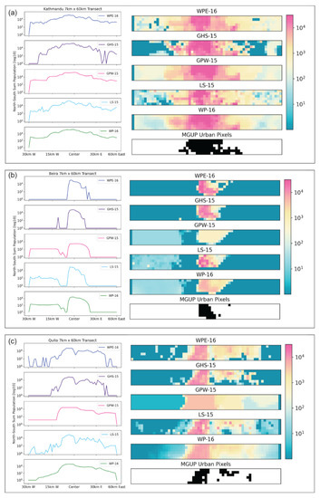
Figure 4.
Transects (7 km by 61 km) of population estimates for each gridded population product centered on urban cores for (a) Kathmandu, (b) Beiria, Mozambique, and (c) Quito. MGUP urban/rural delineation is indicated for each pixel in the transect in the bottom of the plot of each panel. Note that the population sums presented in the line plots are the summation of 7 north-south pixels along the 61 km west-east transect. The color bar corresponds to log10 pixel-level population counts for the transects shown.
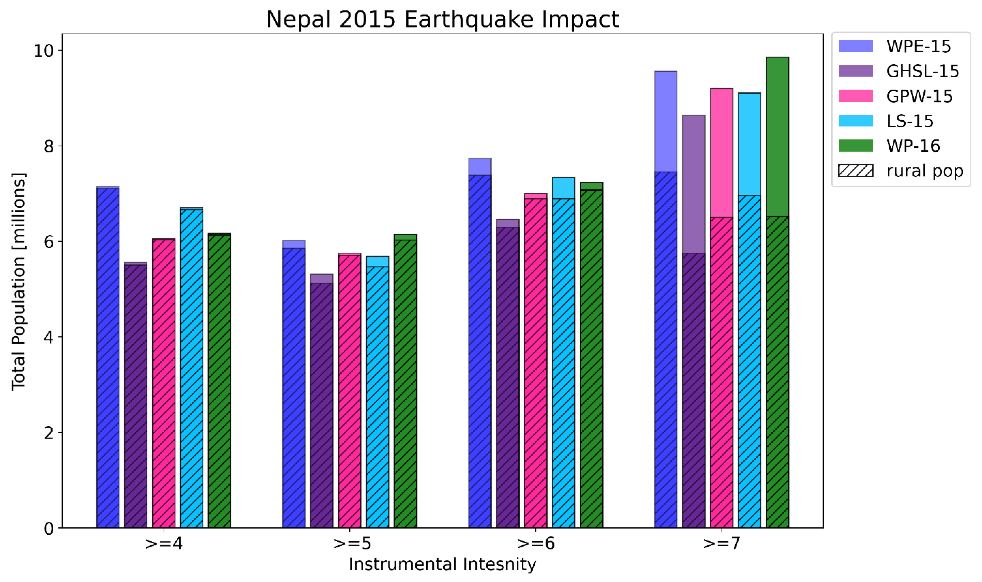
Figure 5 presents the comparison of population estimates exposed to seismic intensity across the five gridded population products, stratified by MGUP-identified urban and rural settlements in Nepal. For the total population exposed to an intensity greater than seven, the difference between the highest and lowest populations estimated to be exposed by the products was more than 1 million people. WP-15 estimated the maximum number of people exposed at 9.85 million people, whereas GHS-15 finds 8.64 million people. The products furthermore measured a wide range in both the total number and the proportion of urban populations exposed to an intensity > 7. On the low end, WPE-16 categorized 22% (2.11 million people) of the population exposed to an intensity greater than 7 as urban, whereas, on the high end, WP-16 indentifed 33% (3.33 million people) of the total population exposed to an intensity greater than 7 as urban. As such, the elevated number of urban residents exposed according to WP-16 paralleled the previous finding that WP-16 identified more urban residents in Nepal compared to the other gridded population products (Table 2).

Figure 5.
The total population impacted by the 2015 earthquake that struck Nepal estimates by “instrumental intensity” for five gridded population datasets. Hatching on bars signifies rural populations, with unhatched portions corresponding to MGUP-identified urban populations.
For intensities less than 7 (Figure 5), we found a broad range of population estimates across the gridded population products. For example, for an intensity between 5 and 6, WPE-16 measured more than 7.73 million people exposed, yet GHS-15 found only 6.46 million people exposed. Generally, the gridded products were largely in agreement for these lower intensities that the vast majority of people impacted lived in rural areas, although LS-15 still identified nearly 500,000 urban residents exposed to an intensity between 5 and 6, and 200,000 urban residents exposed to an intensity between 4 and 5.
3.1.1. Cyclone Idai Exposure in MMZ
Generally, for Cyclone Idai, estimates of populations exposed to high wind speeds and living in flood-inundated areas in MMZ varied across the five gridded population data products, both in total agreement and divided by MGUP-identified urban and rural areas (Figure 6). Wind speeds of 60 km/h, though the least severe of wind categories, had the greatest variation. For instance, WPE-16 measured 7.41 million people (80% rural), the most impacted by wind speeds of 60 km/h. GPW-15 identified only 7.01 million people (88% rural) exposed. Estimates of populations exposed to wind speeds of 120 km/h and flood-inundated areas, the most damaging hazards, also showed substantial variation. Again, WPE-16 ranked first, with 2.39 million people (83% rural) exposed to wind speeds of 120 km/h. The other four gridded products had similar estimates of the total population exposed to wind speeds of 120 km/h, which ranged from 1.89 to 1.95 million people, though GHS-15 and LS-15 identify a greater proportion of urban populations impacted compared to GPW-15 and WP-16. Similarly, estimates of populations living in flood-inundated areas ranged from WPE-16 identifying 817,000 people (88% rural) to GPW-15 identifying 1.28 million people (99% rural). Only for wind speeds of 90 km/h were the products relatively consistent—rural populations were almost exclusively exposed, with high-end estimates of 1.56 million people by WPE-16 and a low-end estimate of 1.46 million people by WP-16.
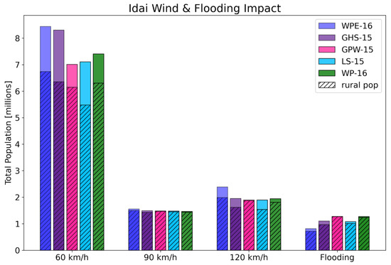
Figure 6.
The total population impacted by wind speeds and flooding from Cyclone Idai across MMZ estimated by five gridded population datasets. Hatching on bars signifies rural populations, with unhatched portions corresponding to MGUP-identified urban populations.
3.1.2. Flash Flood Susceptibility in Ecuador
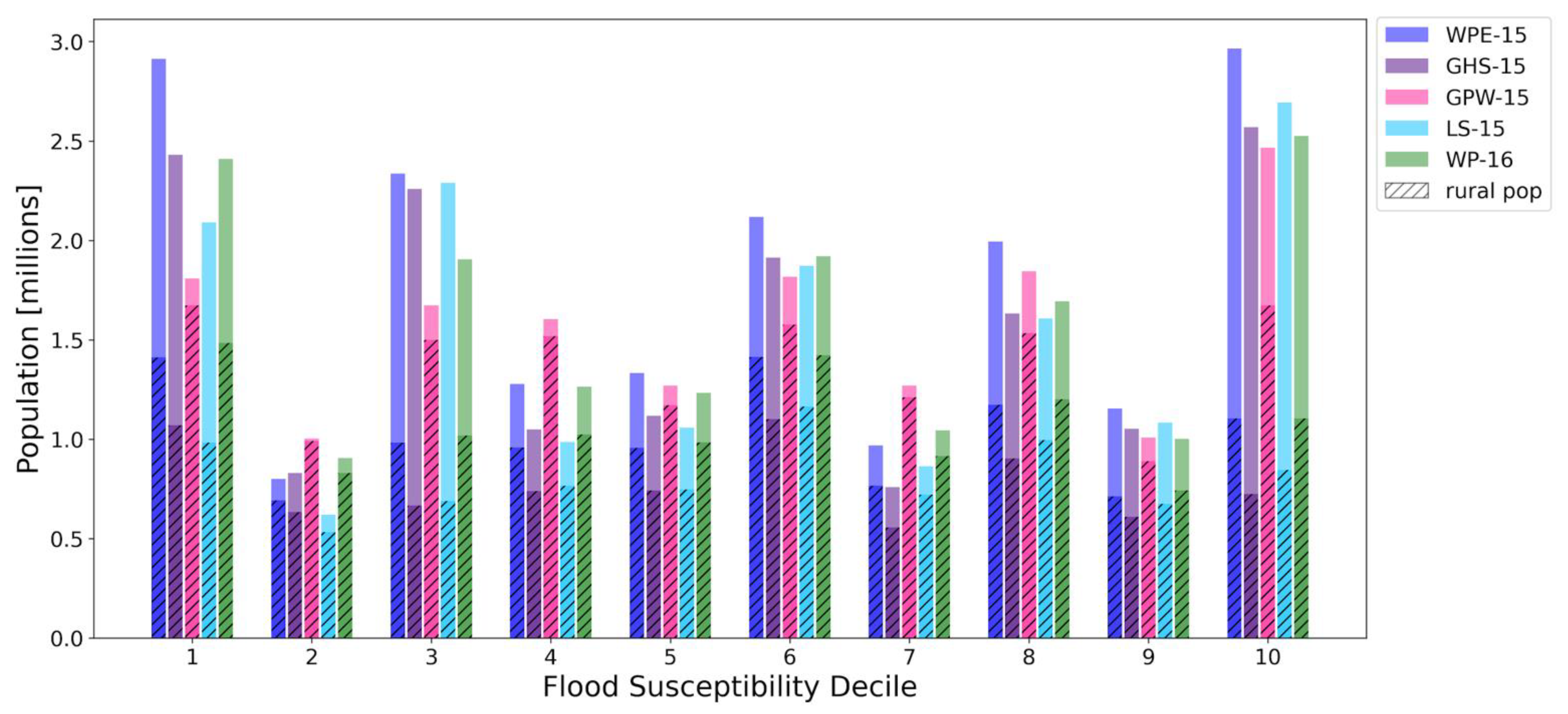
We found two main trends in the comparative analysis of population datasets and the estimation of the rural and urban share within each susceptibility decile (Figure 7). First, for most deciles, WPE-15 identified more population compared to the other four gridded population data products. For example, for the 10th decile, which was the most populated, WPE-15 estimated 2.96 million people, while on the low end, GPW-15 identified 2.47 million people. Second, across all susceptibility deciles GPW-15 estimated a greater share of rural population compared to the other four gridded population datasets. This is demonstrated by clear differences in rural/urban proportions in decile 3, whereby GPW-15 estimated almost all population as rural, compared to the under 50% estimation of rural population identified using the other products. GHS-15 and LS-15, on the other hand, allocated a greater share of population to urban areas. Again, using the 10th decile as an example, which indicates the areas with the highest likelihood of flash flood susceptibility, GHS-15 and LS-15 allocate 72% and 69% of the total population to urban areas, respectively. WPE-15 (62% urban) and WP-16 (56% urban) tend to fall between the preference of GHS-15 and LS-15 for urban areas and GPW-15’s (32% urban) preference for rural areas.
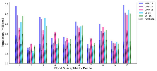
Figure 7.
The total population susceptible to flash floods in Ecuador by susceptibility decile estimated derived from five gridded population datasets. Hatching on bars signifies rural populations, with unhatched portions corresponding to MGUP-identified urban populations.
4. Discussion
Gridded population data provide valuable population counts and densitity estimates for regions in the world where census data is lacking, coarse-scaled, or outdated [13]. The comparable and consistent means by which individual gridded data products are created ensures simple integration with other geospatial data products for use in measuring and monitoring various SDG indicators. However, using SDG 11.5 and a hazard context for three different geographies, we demonstrate that gridded population estimates can vary widely depending on the product of choice. Given the broad geographic contexts of our three case studies, our results suggest that gridded population products will similarly vary across many low- and middle-income countries (LMICs).
While variation in gridded population datasets has been documented by previous studies [21,22,23,24], many widely cited hazards studies (e.g., [64,65]), recent media narratives [66], and United Nations reports [67] continue to employ a single gridded population dataset without justification. In all of these cases, the authors neglect to acknowledge the wide variation in pixel-level population estimates. Indeed, we note that a recent review of estimates of population exposure to sea-level rise or living in low-elevation coastal zones [68] identified multiple global studies published since 2016 that use gridded population products. None of these studies employed multiple gridded population products in their risk estimates. Single-source population estimates, if framed in the context of hazard risk reduction related to SDG 11.5, are thus presented as facts to decision makers. This has broad implications for the allocation of scarce resources. If deployed in the immediate aftermath of a natural disaster, it could also affect humanitarian response and allocation of disaster relief.
Take two examples: first, we found that GHS-15 and LS-15 tend to allocate a greater share of population to the MODIS global urban extent product (MGUP)-designated urban areas compared to the other three products. While the MGUP rural-urban delineation is specific to the context of MODIS built-environment detection [62], and it is not the only criterion to identify urban settlement locations with EO data [25,29], this finding suggests that GHS-15 and LS-15 also prioritize allocating population to where the built environment is detected by Earth observation (EO)-derived spatial correlates. WP-16 also has been shown to prioritize built environment [69]; but our results indicate that WP-16 allocates population more evenly across land cover classes. Second, WPE-16 estimates a far greater population in Nepal, MMZ, and Ecuador compared to both UN estimates (Table 1) [1] and the other gridded population products. Should decision makers be presented with hazard risk reduction solutions or disaster preparedness scenarios based on GHS-15, they may implement policies that overly support urban populations. Communities not easily identified by the spectral signature of the EO-based data product would then be neglected. Similarly, relying only on WPE-16, in which population estimates are largely driven by leveraging the Landsat archive, may overestimate populations exposed or impacted by a hazard, leading to the over-allocation of resources, compared to policies developed with the other gridded population products. As such, efforts to monitor SDG indicators like SDG 11.5, which depend on detailed population data, can vary as a function of the gridded population product employed.
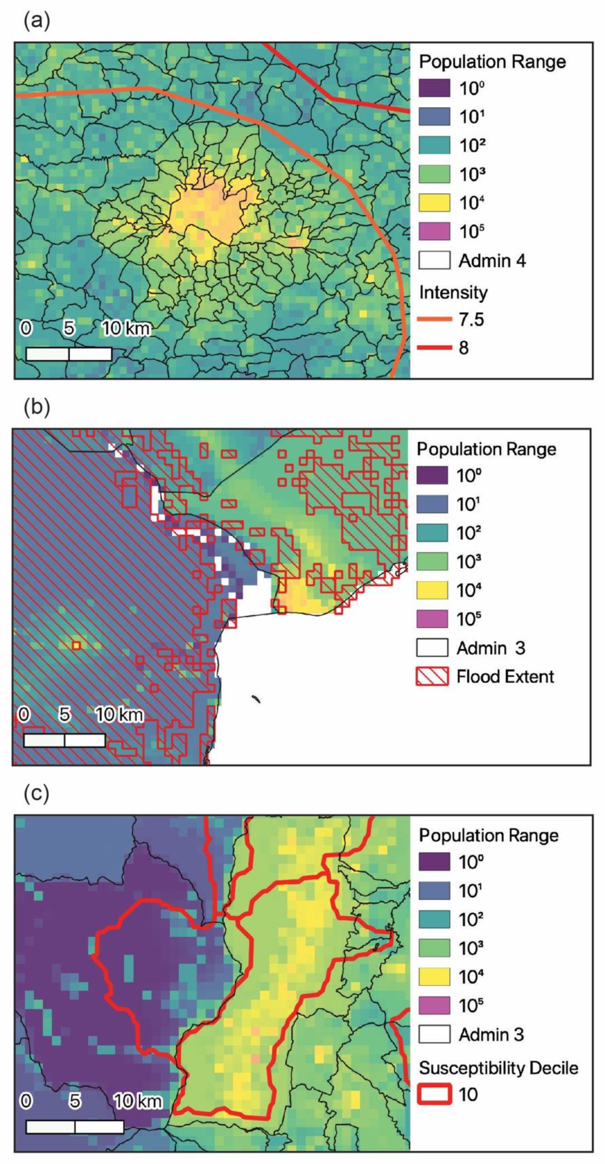
It is important to note that tracking any SDG indicator will also depend on the granularity of hazard data used in association with gridded population data. Indeed, in the context of SDG 11.5 the granularity of hazard data will affect estimates. For example, when we zoomed in on major urban centers from the three case studies presented (Figure 4, Figure 8), significant pixel-level population ranges are identified that may not actually affect the total population measured over larger geographic areas. The USGS earthquake instrument intensity data (Figure 8a) is at a much coarser granularity over Kathmandu than the EO-observed flood inundated area around Beira, Mozambique (Figure 8b), or the flash flood susceptibility layer for Quito (Figure 8c). Yet, unlike the more standardized analysis-ready hazard datasets we presented here, there is not a widely accepted set of criteria for deciding which gridded population dataset should be used to measure exposure to a given hazard.

Figure 8.
Pixel-level population range (maximum–minimum population estimated across gridded population products) overlaid with administrative units used for deriving gridded population datasets and the hazard under study. Panel (a) is situated over Kathmandu, with the earthquake instrument intensity contours shown. Panel (b) covers Quito with the highest flash flood sustainability area outlined in red. Panel (c) focuses on Beira, Mozambique and the mouth of the Pungwe River. Red hatching is the 90 m flood layer from Cyclone Idai resampled to 1 km.
While recent “fitness for use” guidelines provide key information for researchers, practitioners, and decision makers [5,20], our results suggest that the single use of a gridded population product should be avoided in tracking SDG indicators. These guidelines emphasize that spatial scale, reliability, and granularity of underlying census data, the population under study, and geography must be considered in data selection. Yet the variation across gridded population products we found for a range of hazards across geographic contexts signals that the single use of a product has realworld financial consequences. For instance, using our results from Cyclone Idai and per capita dollar basic disaster emergency costs of $112 per person [70], relief costs solely for those in flood inundated areas in MMZ range from US$92 million using the WPE-16 estimate of 817,000 people to US$143 million using GHS-15 estimate 1.28 million. Both estimates are below the official estimate of 1.85 million people impacted by Idai and the immediate financial estimate of US$300 million [43]. As such, we caution against the single use of a gridded population product. We reaffirm the need for the validation of existing products and urge future producers of gridded population products to provide error estimations.
Different gridded population modeling approaches and EO input data can result in varying population estimates per grid cell [20]. However, the finer the spatial resolution of input administrative units (Table 2) associated with population counts, the more similar the output population values per pixel will be across products regardless of the disaggregation approach. This is clear from Figure 4a, which shows much less variation in population estimates across the urban-rural gradient around Kathmandu. Generally speaking, finer administrative units tend to concentrate in higher population density areas. Administrative units that are larger, and coarser in spatial extent, tend to associate with lower population density areas, and are affected more by the different disaggregation approaches and their underlying assumptions. The result is greater variation in population estimates per pixel within the same administrative unit. We thus encourage national census agencies to release data with associated boundary files for the highest resolution units possible.
Our results further highlight differences between constrained and unconstrained gridded populations products. Constrained approaches disaggregate population counts linked to administrative units only within pixels identified as “settled.” In doing so, there may be a tendency to overestimate the number of people “distributed” within high-density (urban) settings. Our results indicate that this is the case with GHS-15. In contrast, the unconstrained approach will disaggregate population counts into any pixel identified as “land,” which may overestimate the number of people allocated within low-density, i.e., more rural, settings. In the case of GPW-15, the overestimation in low-density (rural) settings is expected to be even more pronounced than in the other unconstrained products given that the disaggregated population totals are evenly redistributed within all pixels identified as “land” and there is no additional ancillary data used in the model.
While we recommend using multiple products in hazard analysis, if selecting a single gridded population product, it is important to identify not only if the gridded population product is constrained in some way, but also how it is constrained. Underlying data sources of constrained products may have validation or uncertainty estimates that may vary by region or time point. For input settlement products that represent the constrained “built” areas in which population counts are disaggregated, there is a general expectation that those gridded products will have a more accurate representation of population distribution. However, the final gridded population product will be greatly impacted by the presence of omission and commission errors in the input settlement dataset, with small/isolated rural settlements potentially being more difficult to detect and certain types of land cover (e.g., rock outcrops or sandy soils) potentially being misclassified as settlement areas [71].
On the other hand, unconstrained approaches use a dasymetric approach to disaggregate input administrative population values within all pixels identified as “land.” This will introduce error in the final gridded output for those areas that are actually uninhabited. There will be some trade-off with a minimization of the presence of omission and commission errors in whatever input settlement data is used in the modeling due to the influence of other ancillary covariates representing factors correlated with population density and presence. There is error in all products, but some basic understanding of how the gridded data products are produced can help identify which product makes the most sense for a given application. Reed et al. (2018) [72] demonstrates the relative robustness of the unconstrained WorldPop dataset compared to the constrained HRSL dataset. The similarities in error metrics for these products emphasizes the importance of considering omission/commission errors in the input built datasets and subsequent allocation of population values in the final product.
Finally, it should be noted that most of these gridded population datasets represent a residential population, or where people are most likely to be when at home. LandScan is an exception and represents the ambient population, or the average population distribution over 24 h. That type of data product is potentially useful for assessing exposure as it represents not only the static census-based residence information but also the ambient nature of population movement over a 24 h period.
5. Conclusions
Vector-based administrative-level population data often fails to disaggregate population at the spatial scales requisite to identify where people actually live on the planet. This type of data can fail to provide useful information for the delivery of services required to achieve the SDGs. As such, our findings reinforce the many advantages of using gridded population products to track SDG indicators. This is especially important in the context of measuring, monitoring, and mapping SDG 11.5. Indeed, reducing exposure to hazards requires accurate population estimates, and for many LMICs, Earth observation-derived gridded population products are the best available data. Likewise, gridded population products can provide crucial information in post-disaster contexts as well. The case studies we showcase here reinforce the broad utility of these products and advance our understanding of “fitness for use” for both SDG 11.5 and the 73 SDG indicators that require accurate, comparable, and timely high-resolution population estimates.
Nonetheless, we highlight that for some geographical regions (and/or hazards), population estimates will vary depending on the choice of gridded population product. Despite the variation we identify across gridded population datasets, we emphasize that uncertainty is not per se a limitation in employing gridded population datasets to track the SDGs. Without externally derived validation data or producer error metrics, it remains difficult to provide definitive recommendations in terms of what product to use, where and for what type of hazard. As such, we recommend further resources be dedicated to micro census data collection and encourage producers to quantify uncertainty in future gridded population products.
Most importantly, we recommend that researchers, practitioners, and decision makers acknowledge that inherent uncertainty when using these products. Along with leveraging the “fitness for use guidelines” [5,20], a key step to doing so is to perform a sensitivity analysis [23] and/or present a range of estimates using multiple gridded populations using an ensemble approach. To this end, we have provided the code used in the analysis and made available a global raster dataset that allows for the intercomparison of gridded population products. Furthermore, researchers and practitioners who develop tools for decision makers to track the SDGs should incorporate multiple gridded population datasets. Decision makers can thus develop policies and allocate resources informed by information that captures some of the inherent uncertainties of leveraging EO data to measure human populations across the planet. Indeed, single-use population estimates could open the door for bad actors to select the gridded population product that maximizes progress towards achieving an SDG. Lastly, we emphasize that the development of indicators, including the use of datasets like gridded population products, should be a collective effort between users and producers across decision-making levels [73].
Supplementary Materials
The following are available online at https://www.mdpi.com/article/10.3390/su13137329/s1.
Author Contributions
C.T., A.E.G. and A.d.S. developed the concept for the paper. C.T. wrote all code, performed all analysis, and produced all figures. C.T., A.E.G., A.S., A.d.S. drafted the initial text. A.B., C.H. (Carolynne Hultquist), and A.K. developed the Ecuador flood susceptibility layer. F.S. and G.Y. assisted with gridded population data selection, interpretation, and use. C.H. (Charles Huyck) consulted on 2015 Nepal earthquake data selection and interpretation. All authors contributed intellectually to the project throughout and all contributed to the final manuscript text. All authors have read and agreed to the published version of the manuscript.
Funding
C.T. was supported by the Earth Institute Postdoctoral Research Fellowship Program. A.B., C.H. (Carolynne Hultquist) and A.K. were supported by NASA Grant #80NSSC18K0342. A.S. was supported by funding from the Bill & Melinda Gates Foundation (OPP1134076 and 3(PG009268-05)). C.T., A.E.G., F.S., A.d.S. and G.Y. were supported by NASA Grant #80NSSC18K0328 for “Population and Infrastructure on Our Human Planet: Supporting Sustainable Development through Improved Spatial Data and Models for Human Settlements, Infrastructure and Population”.
Institutional Review Board Statement
Not applicable.
Informed Consent Statement
Not applicable.
Data Availability Statement
All code and data are available at: https://github.com/cascadet/PopGridCompare (accessed on 20 January 2021).
Acknowledgments
We thank three anonamous reviewers for their valuable feedback.
Conflicts of Interest
The authors declare no conflict of interest.
References
- UN-DESA. Sustainable Development Goals. Available online: https://sdgs.un.org/goals (accessed on 1 March 2021).
- Sachs, J.D. From millennium development goals to sustainable development goals. Lancet 2012, 379, 2206–2211. [Google Scholar] [CrossRef]
- Griggs, D.J.; Nilsson, M.; Stevance, A.; McCollum, D. (Eds.) A Guide to SDG Interactions: From Science to Implementation; International Council for Science (ICSU): Paris, France, 2017; Available online: https://council.science/wp-content/uploads/2017/05/SDGs-Guide-to-Interactions.pdf (accessed on 20 January 2021).
- Attaran, A. An immeasurable crisis? A criticism of the millennium development goals and why they cannot be measured. PLoS Med. 2005, 2, e318. [Google Scholar] [CrossRef] [Green Version]
- Thematic Research Network on Data and Statistics (TReNDS). Leaving No One Off the Map: A Guide for Gridded Population Data for Sustainable Development. 2020. Available online: https://static1.squarespace.com/static/5b4f63e14eddec374f416232/t/5eb2b65ec575060f0adb1feb/1588770424043/Leaving+no+one+off+the+map-4.pdf (accessed on 20 January 2021).
- About the Global Partnership for Sustainable Development Data. Available online: https://www.data4sdgs.org/index.php/about-gpsdd (accessed on 1 March 2021).
- Avtar, R.; Aggarwal, R.; Kharrazi, A.; Kumar, P.; Kurniawan, T.A. Utilizing geospatial information to implement SDGs and monitor their Progress. Environ. Monit. Assess. 2019, 192, 35. [Google Scholar] [CrossRef] [PubMed]
- Kavvada, A.; Metternicht, G.; Kerblat, F.; Mudau, N.; Haldorson, M.; Laldaparsad, S.; Friedl, L.; Held, A.; Chuvieco, E. Towards delivering on the sustainable development goals using earth observations. Remote Sens. Environ. 2020, 247, 111930. [Google Scholar] [CrossRef]
- Kussul, N.; Lavreniuk, M.; Kolotii, A.; Skakun, S.; Rakoid, O.; Shumilo, L. A workflow for sustainable development goals indicators assessment based on high-resolution satellite data. Int. J. Digit. Earth 2020, 13, 309–321. [Google Scholar] [CrossRef]
- Estoque, R.C. A review of the sustainability concept and the state of SDG monitoring using remote sensing. Remote Sens. 2020, 12, 1770. [Google Scholar] [CrossRef]
- Kavvada, A.; Held, A. Analysis-ready earth observation data and the united nations sustainable development goals. In Proceedings of the IGARSS 2018—2018 IEEE International Geoscience and Remote Sensing Symposium, Valencia, Spain, 22–27 July 2018; pp. 434–436. [Google Scholar]
- De Lamo, X.; Simonson, W. Earth Observation for SDG: Compendium of Earth Observation Contributions to the SDG Targets and Indicators. ESA. May 2020. Available online: https://eo4society.esa.int/wp-content/uploads/2021/01/EO_Compendium-for-SDGs.pdf (accessed on 20 January 2021).
- Wardrop, N.A.; Jochem, W.C.; Bird, T.J.; Chamberlain, H.R.; Clarke, D.; Kerr, D.; Bengtsson, L.; Juran, S.; Seaman, V.; Tatem, A.J. Spatially disaggregated population estimates in the absence of national population and housing census data. Proc. Natl. Acad. Sci. USA 2018, 115, 3529–3537. [Google Scholar] [CrossRef] [Green Version]
- Juran, S.; Broer, P.N.; Klug, S.J.; Snow, R.C.; Okiro, E.; Ouma, P.O.; Snow, R.; Tatem, A.J.; Meara, J.G.; Alegana, V.A. Geospatial mapping of access to timely essential surgery in sub-Saharan Africa. BMJ Glob. Health 2018, 3, e000875. [Google Scholar] [CrossRef] [Green Version]
- Dotse-Gborgbortsi, W.; Dwomoh, D.; Alegana, V.; Hill, A.; Tatem, A.J.; Wright, J. The influence of distance and quality on utilisation of birthing services at health facilities in Eastern Region, Ghana. BMJ Glob. Health 2019, 4, e002020. [Google Scholar] [CrossRef] [Green Version]
- Palacios-Lopez, D.; Bachofer, F.; Esch, T.; Marconcini, M.; MacManus, K.; Sorichetta, A.; Zeidler, J.; Dech, S.; Tatem, A.; Reinartz, P. High-resolution gridded population datasets: Exploring the Capabilities of the world settlement footprint 2019 imperviousness layer for the African continent. Remote Sens. 2021, 13, 1142. [Google Scholar] [CrossRef]
- Melchiorri, M.; Pesaresi, M.; Florczyk, A.J.; Corbane, C.; Kemper, T. Principles and applications of the global human settlement layer as baseline for the land use efficiency indicator—SDG 11.3.1. ISPRS Int. J. Geo Inf. 2019, 8, 96. [Google Scholar] [CrossRef] [Green Version]
- Qiu, Y.; Zhao, X.; Fan, D.; Li, S. Geospatial disaggregation of population data in supporting SDG assessments: A case study from Deqing county, China. ISPRS Int. J. Geo Inf. 2019, 8, 356. [Google Scholar] [CrossRef] [Green Version]
- Schiavina, M.; Melchiorri, M.; Corbane, C.; Florczyk, A.; Freire, S.; Pesaresi, M.; Kemper, T. Multi-scale estimation of land use efficiency (SDG 11.3.1) across 25 years using global open and free data. Sustain. Sci. Pract. Policy 2019, 11, 5674. [Google Scholar] [CrossRef] [Green Version]
- Leyk, S.; Gaughan, A.E.; Adamo, S.B. The spatial allocation of population: A review of large-scale gridded population data products and their fitness for use. Earth Syst. Monit. 2019. Available online: https://www.earth-syst-sci-data.net/11/1385/2019/essd-11-1385-2019-discussion.html (accessed on 20 January 2021). [CrossRef] [Green Version]
- Archila Bustos, M.F.; Hall, O.; Niedomysl, T.; Ernstson, U. A pixel level evaluation of five multitemporal global gridded population datasets: A case study in Sweden, 1990–2015. Popul. Environ. 2020, 42, 255–277. [Google Scholar] [CrossRef]
- Chen, R.; Yan, H.; Liu, F.; Du, W.; Yang, Y. Multiple global population datasets: Differences and spatial distribution characteristics. ISPRS Int. J. Geo Inf. 2020, 9, 637. [Google Scholar] [CrossRef]
- Smith, A.; Bates, P.D.; Wing, O.; Sampson, C.; Quinn, N.; Neal, J. New estimates of flood exposure in developing countries using high-resolution population data. Nat. Commun. 2019, 10, 1814. [Google Scholar] [CrossRef] [PubMed] [Green Version]
- Fries, B.F.; Guerra, C.A.; García, G.A.; Wu, S.L.; Smith, J.M.; Oyono, J.N.M.; Donfack, O.T.; Nfumu, J.O.O.; Hay, S.I.; Smith, D.L.; et al. Measuring the accuracy of gridded human population density surfaces: A case study in Bioko Island, Equatorial Guinea. Cold Spring Harb. Lab. 2020. [Google Scholar] [CrossRef]
- Tuholske, C.; Caylor, K.; Evans, T.; Avery, R. Variability in urban population distributions across Africa. Environ. Res. Lett. 2019, 14, 85009. [Google Scholar] [CrossRef]
- Green, H.K.; Lysaght, O.; Saulnier, D.D.; Blanchard, K.; Humphrey, A.; Fakhruddin, B.; Murray, V. Challenges with disaster mortality data and measuring progress towards the implementation of the sendai framework. Int. J. Disaster Risk Sci. 2019, 10, 449–461. [Google Scholar] [CrossRef] [Green Version]
- Mizutori, M. Reflections on the sendai framework for disaster risk reduction: Five years since its adoption. Int. J. Disaster Risk Sci. 2020, 11, 147–151. [Google Scholar] [CrossRef] [Green Version]
- Dagys, K. The Effectiveness of Forecast-Based Humanitarian Assistance in Anticipation of Extreme Winters: Evidence from an Intervention for Vulnerable Herders in Mongolia. 2020. Available online: https://www.researchgate.net/profile/Kadirbyek_Dagys/publication/347885328_The_effectiveness_of_forecast-based_humanitarian_assistance_in_anticipation_of_extreme_winters_Evidence_from_an_intervention_for_vulnerable_herders_in_Mongolia/links/5fe570d0a6fdccdcb8fc06a2/The-effectiveness-of-forecast-based-humanitarian-assistance-in-anticipation-of-extreme-winters-Evidence-from-an-intervention-for-vulnerable-herders-in-Mongolia.pdf (accessed on 2 March 2021).
- Cattaneo, A.; Nelson, A. Global mapping of urban–rural catchment areas reveals unequal access to services. Proc. Natl. Acad. Sci. USA 2021. Available online: https://www.pnas.org/content/118/2/e2011990118.short (accessed on 1 June 2021). [CrossRef] [PubMed]
- Frye, C.; Wright, D.J.; Nordstrand, E.; Terborgh, C.; Foust, J. Using classified and unclassified land cover data to estimate the footprint of human settlement. Data Sci. J. 2018, 17. Available online: https://datascience.codata.org/articles/10.5334/dsj-2018-020/?toggle_hypothesis=on (accessed on 20 January 2021). [CrossRef]
- Florczyk, A.J.; Corbane, C.; Ehrlich, D.; Freire, S.; Kemper, T.; Maffenini, L.; Melchiorri, M.; Pesaresi, M.; Politis, P.; Schiavina, M.; et al. GHSL Data Package 2019; JRC Technical Report: Luxembourg, 2019. [Google Scholar] [CrossRef]
- NASA Socioeconomic Data and Applications Center (SEDAC). Gridded Population of the World, Version 4; (GPWv4): Population Density Adjusted to Match 2015; NASA Socioeconomic Data and Applications Center (SEDAC): Palisades, NY, USA, 2018. [Google Scholar]
- LandScan. LandScan Datasets, LandScanTM. Available online: https://landscan.ornl.gov/index.php/landscan-datasets (accessed on 24 February 2019).
- Worldpop. WorldPop: Population. 18 November 2016. Available online: https://www.worldpop.org/doi/10.5258/SOTON/WP00004 (accessed on 24 February 2019).
- POPGRID. Input Layers for Global Gridded Data Sets. 2019. Available online: https://www.popgrid.org/data-docs-table2 (accessed on 24 February 2019).
- UN-DESA. World Urbanization Prospects 2018. Available online: https://esa.un.org/unpd/wup/ (accessed on 30 August 2018).
- Stevens, F.R.; Gaughan, A.E.; Linard, C.; Tatem, A.J. Disaggregating census data for population mapping using random forests with remotely-sensed and ancillary data. PLoS ONE 2015, 10, e0107042. [Google Scholar] [CrossRef] [PubMed] [Green Version]
- Dobson, J.E.; Bright, E.A.; Coleman, P.R.; Durfee, R.C.; Worley, B.A. LandScan: A global population database for estimating populations at risk. Photogramm. Eng. Remote Sens. 2000, 66, 849–857. [Google Scholar]
- USGS. M 7.8–36 km E of Khudi, Nepal. In Earthquake Hazards Program. Available online: https://earthquake.usgs.gov/earthquakes/eventpage/us20002926/executive (accessed on 4 March 2021).
- Hall, M.L.; Lee, A.C.K.; Cartwright, C.; Marahatta, S.; Karki, J.; Simkhada, P. The 2015 Nepal earthquake disaster: Lessons learned one year on. Public Health 2017, 145, 39–44. [Google Scholar] [CrossRef] [PubMed]
- Reid, K. 2015 Nepal Earthquake: Facts, FAQs, and How to Help. World Vision. 2018. Available online: https://www.worldvision.org/disaster-relief-news-stories/2015-nepal-earthquake-facts (accessed on 4 March 2021).
- Government of Nepal National Planning Commission, Kathmandu. Nepal Earthquake 2015 Post Disaster Needs Assessment Vol. B: Sector Reports. 2015. Available online: https://www.npc.gov.np/images/category/PDNA_volume_BFinalVersion.pdf (accessed on 20 January 2021).
- Ocha, U.N. Humanitarian Response Plan 2018–2019 (Revised Following Cyclone Idai, March 2019); United Nations Office for the Coordination of Humanitarian Affairs Mozambique. Available online: https://reliefweb.int/sites/reliefweb.int/files/resources/ROSEA_20190325_MozambiqueFlashAppeal.pdf (accessed on 20 January 2021).
- World Food Program. Mozambique Satellite Detected Waters, Cyclone Idai. 2019. Available online: https://data.humdata.org/dataset/mozambique-flood-detected-waters-cyclone-idai (accessed on 20 January 2021).
- EC-JRC. Overall Red Tropical Cyclone Alert for IDAI-19 in Mozambique, Zimbabwe, Miscellaneous (French) Indian Ocean Islands from 09 March 2019 06:00 UTC to 15 March 2019 00:00 UTC; Global Disaster Alert and Coordination System. Available online: https://www.gdacs.org/resources.aspx?eventid=1000552&episodeid=24&eventtype=TC (accessed on 20 January 2021).
- Ahern, M.; Kovats, R.S.; Wilkinson, P.; Few, R.; Matthies, F. Global health impacts of floods: Epidemiologic evidence. Epidemiol. Rev. 2005, 27, 36–46. [Google Scholar] [CrossRef] [PubMed] [Green Version]
- Montz, B.E.; Gruntfest, E. Flash flood mitigation: Recommendations for research and applications. Glob. Environ. Chang. Part B Environ. Hazards 2002, 4, 15–22. [Google Scholar] [CrossRef]
- Hallegatte, S.; Green, C.; Nicholls, R.J.; Corfee-Morlot, J. Future flood losses in major coastal cities. Nat. Clim. Chang. 2013, 3, 802–806. [Google Scholar] [CrossRef]
- SENPLADES. Boletín Informativo Costos de las Pérdidas por las Inundaciones, mes de Julio. 2012. Available online: https://reliefweb.int/sites/reliefweb.int/files/resources/Costos%20de%20las%20perdidas%20por%20las%20inundaciones%202012.pdf (accessed on 20 January 2021).
- Pinos, J.; Orellana, D.; Timbe, L. Assessment of microscale economic flood losses in urban and agricultural areas: Case study of the Santa Bárbara river, Ecuador. Nat. Hazards 2020, 103, 2323–2337. [Google Scholar] [CrossRef]
- Informe a la Nación 2007–2017; Planifica Ecuador Secretaría Técnica; 2017. Report No.: Informe Nacional, 214. Available online: www.planificación.gob.ec (accessed on 20 January 2021).
- Kruczkiewicz, A.; Bucherie, A.; Ayala, F.; Hultquist, C.; Vergara, H.; Mason, S.; Bazo, J.; de Sherbinin, A. Development of a flash flood confidence index from disaster reports and geophysical susceptibility. Remote Sens. 2021, 13. submitted. [Google Scholar]
- Chao, Y.-S.; Wu, C.-J. Principal component-based weighted indices and a framework to evaluate indices: Results from the Medical Expenditure Panel Survey 1996 to 2011. PLoS ONE 2017, 12, e0183997. [Google Scholar] [CrossRef]
- Janizadeh, S.; Avand, M.; Jaafari, A.; Van Phong, T.; Bayat, M.; Ahmadisharaf, E.; Prakash, I.; Pham, B.T.; Lee, S. Prediction success of machine learning methods for flash flood susceptibility mapping in the Tafresh watershed, Iran. Sustain. Sci. Pract. Policy 2019, 11, 5426. [Google Scholar] [CrossRef] [Green Version]
- Pham, B.T.; Avand, M.; Janizadeh, S.; Van Phong, T.; Al-Ansari, N.; Ho, L.; Das, S.; Van Le, H.; Amini, A.; Bozchaloei, S.K.; et al. GIS based hybrid computational approaches for flash flood susceptibility assessment. Water 2020, 12, 683. [Google Scholar] [CrossRef] [Green Version]
- Ullah, K.; Zhang, J. GIS-based flood hazard mapping using relative frequency ratio method: A case study of Panjkora river Basin, eastern Hindu Kush, Pakistan. PLoS ONE 2020, 15, e0229153. [Google Scholar] [CrossRef] [Green Version]
- Azmeri Hadihardaja, I.K.; Vadiya, R. Identification of flash flood hazard zones in mountainous small watershed of Aceh Besar Regency, Aceh Province, Indonesia. Egypt J. Remote Sens. Space Sci. 2016, 19, 143–160. [Google Scholar]
- Saharia, M.; Kirstetter, P.-E.; Vergara, H.; Gourley, J.J.; Hong, Y.; Giroud, M. Mapping flash flood severity in the United States. J. Hydrometeorol. 2017, 18, 397–411. [Google Scholar] [CrossRef]
- Mahmood, S.; Rahman, A.-U. Flash flood susceptibility modelling using geomorphometric approach in the Ushairy basin, eastern Hindu Kush. J. Earth Syst. Sci. 2019, 128. [Google Scholar] [CrossRef] [Green Version]
- Oruonye, E.D. Morphometry and flood in small drainage basin: Case study of Mayogwoi river basin in Jalingo, Taraba state Nigeria. J. Geogr. Environ. Earth Sci. Int. 2016, 5, 1–12. [Google Scholar] [CrossRef]
- Lehner, B.; Verdin, K.; Jarvis, A. New global hydrography derived from spaceborne elevation data. Eos 2008, 89, 93. [Google Scholar] [CrossRef]
- Huang, X.; Huang, J.; Wen, D.; Li, J. An updated MODIS global urban extent product (MGUP) from 2001 to 2018 based on an automated mapping approach. Int. J. Appl. Earth Obs. Geoinf. 2021, 95, 102255. [Google Scholar] [CrossRef]
- Global Human Settlement—Global Definition of Cities, Urban and Rural Areas—European Commission. 6 July 2016. Available online: https://ghsl.jrc.ec.europa.eu/degurba.php (accessed on 30 March 2021).
- Kulp, S.A.; Strauss, B.H. New elevation data triple estimates of global vulnerability to sea-level rise and coastal flooding. Nat. Commun. 2019, 10, 5752. [Google Scholar] [CrossRef] [Green Version]
- Mora, C.; Dousset, B.; Caldwell, I.R.; Powell, F.E.; Geronimo, R.C.; Bielecki, C.R.; Counsell, C.W.W.; Dietrich, B.S.; Johnston, E.T.; Louis, L.; et al. Global risk of deadly heat. Nat. Clim. Chang. 2017, 7, 501. [Google Scholar] [CrossRef]
- Lustgarten, A. The Great Climate Migration Has Begun; The New York Times. 16 December 2020. Available online: https://www.nytimes.com/interactive/2020/07/23/magazine/climate-migration.html (accessed on 6 March 2021).
- Gu, D. Exposure and Vulnerability to Natural Disasters for World’s Cities; UN DESA; 2019. Available online: https://www.un.org/en/development/desa/population/publications/pdf/technical/TP2019-4.pdf (accessed on 20 January 2021).
- McMichael, C.; Dasgupta, S.; Ayeb-Karlsson, S.; Kelman, I. A review of estimating population exposure to sea-level rise and the relevance for migration. Environ. Res. Lett. 2020, 15, 123005. [Google Scholar] [CrossRef] [PubMed]
- Nieves, J.J.; Stevens, F.R.; Gaughan, A.E.; Linard, C.; Sorichetta, A.; Hornby, G.; Patel, N.N.; Tatem, A.J. Examining the correlates and drivers of human population distributions across low- and middle-income countries. J. R. Soc. Interface 2017, 14. [Google Scholar] [CrossRef] [Green Version]
- IFRC. The Cost of Doing Nothing: The Humanitarian Price of Climate Change and How It Can Be Avoided. 2019. Available online: https://media.ifrc.org/ifrc/wp-content/uploads/sites/5/2019/09/2019-IFRC-CODN-EN.pdf (accessed on 20 January 2021).
- Stevens, F.R.; Gaughan, A.E.; Nieves, J.J.; King, A.; Sorichetta, A.; Linard, C.; Tatem, A.J. Comparisons of two global built area land cover datasets in methods to disaggregate human population in eleven countries from the global south. Int. J. Digit. Earth 2020, 13, 78–100. [Google Scholar] [CrossRef]
- Reed, F.J.; Gaughan, A.E.; Stevens, F.R.; Yetman, G.; Sorichetta, A.; Tatem, A.J. Gridded population maps informed by different built settlement products. Data 2018, 3, 33. [Google Scholar] [CrossRef] [Green Version]
- Bell, S.; Morse, S. Breaking through the glass ceiling: Who really cares about sustainability indicators? Local Environ. 2001, 6, 291–309. [Google Scholar] [CrossRef]


Publisher’s Note: MDPI stays neutral with regard to jurisdictional claims in published maps and institutional affiliations. |
© 2021 by the authors. Licensee MDPI, Basel, Switzerland. This article is an open access article distributed under the terms and conditions of the Creative Commons Attribution (CC BY) license (https://creativecommons.org/licenses/by/4.0/).