
Social Vulnerability across the Great Lakes Basin: A County-Level Comparative and Spatial Analysis


Abstract
:1. Introduction
1.1. Social Vulnerability
1.2. Measuring Social Vulnerability
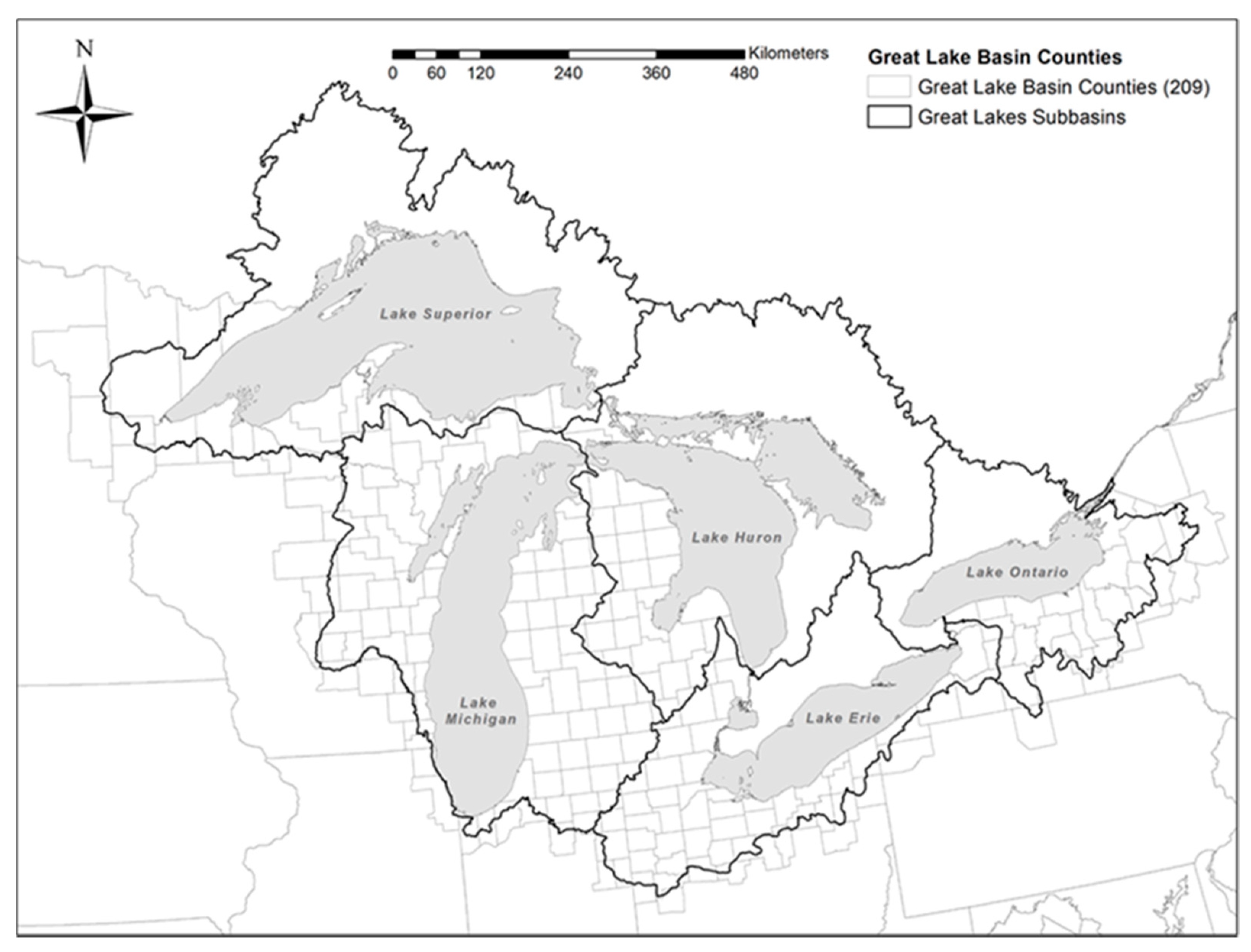
1.3. Great Lakes Context
2. Materials and Methods
2.1. Social Vulnerability
2.1.1. Socioeconomic Status
2.1.2. Household Composition and Disability
2.1.3. Minority Status and Language
2.1.4. Housing Type and Transportation
2.2. Spatial and Statistical Analysis
3. Results
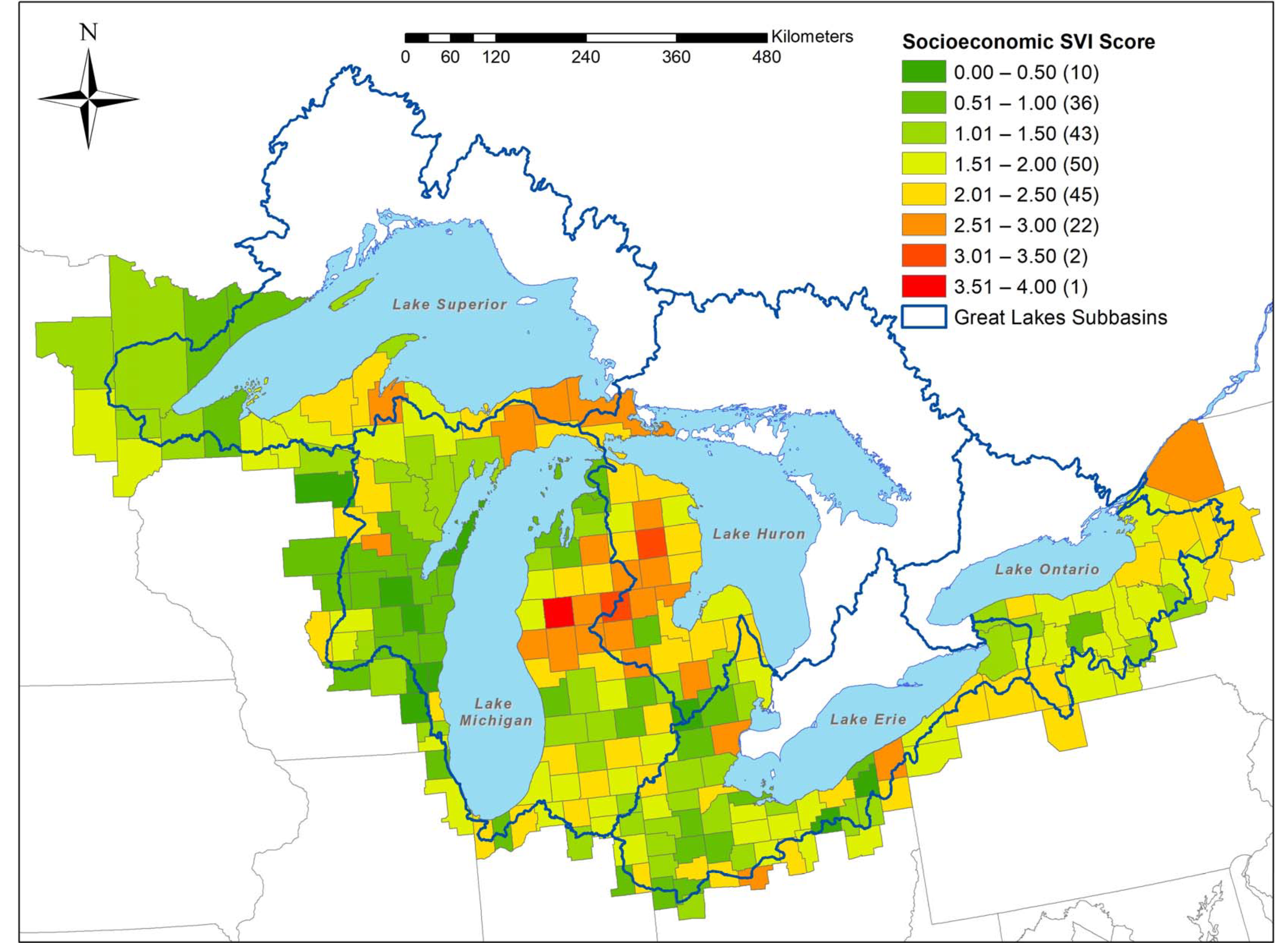
3.1. Socioeconomic Vulnerability
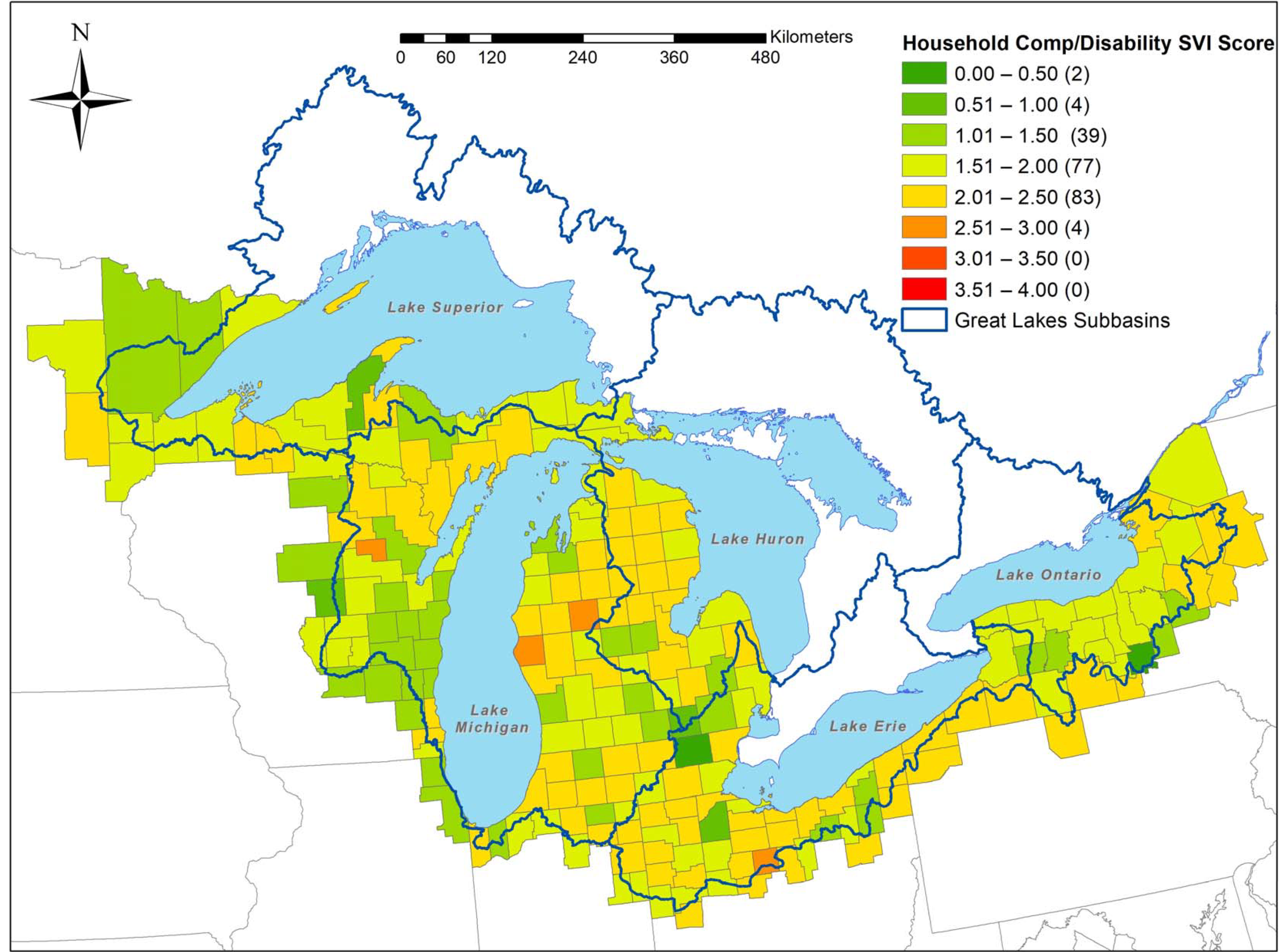
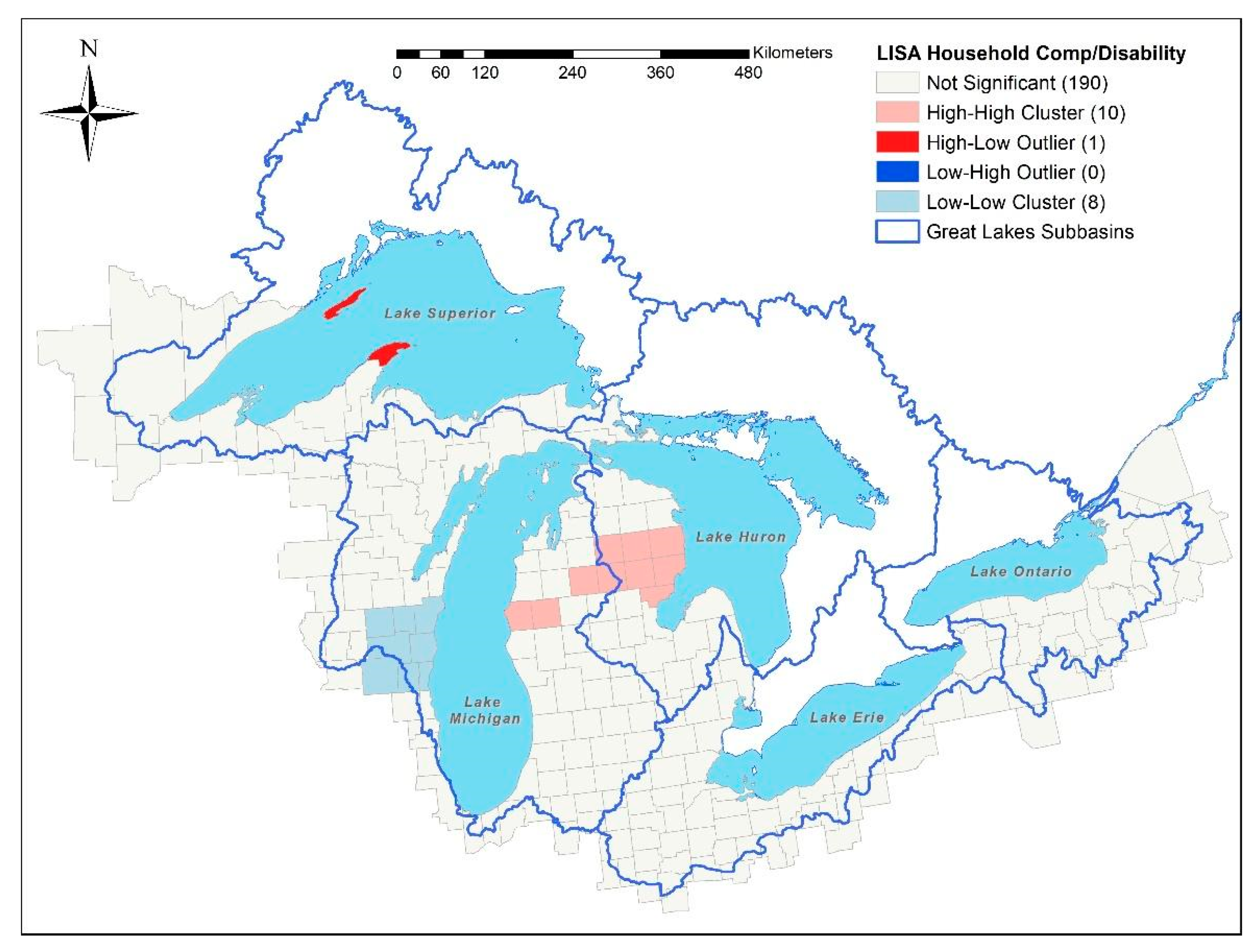
3.2. Household Composition and Disability
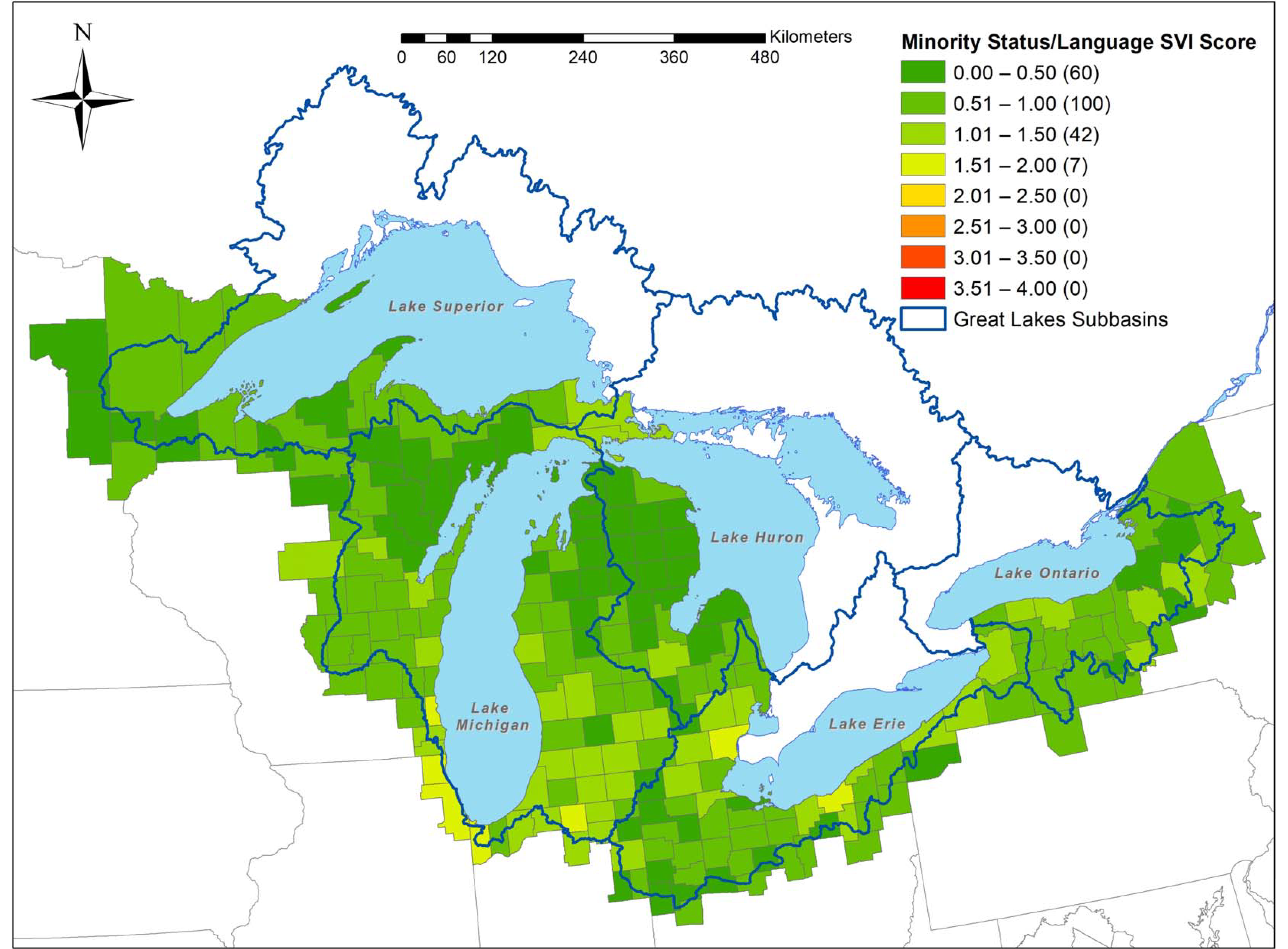
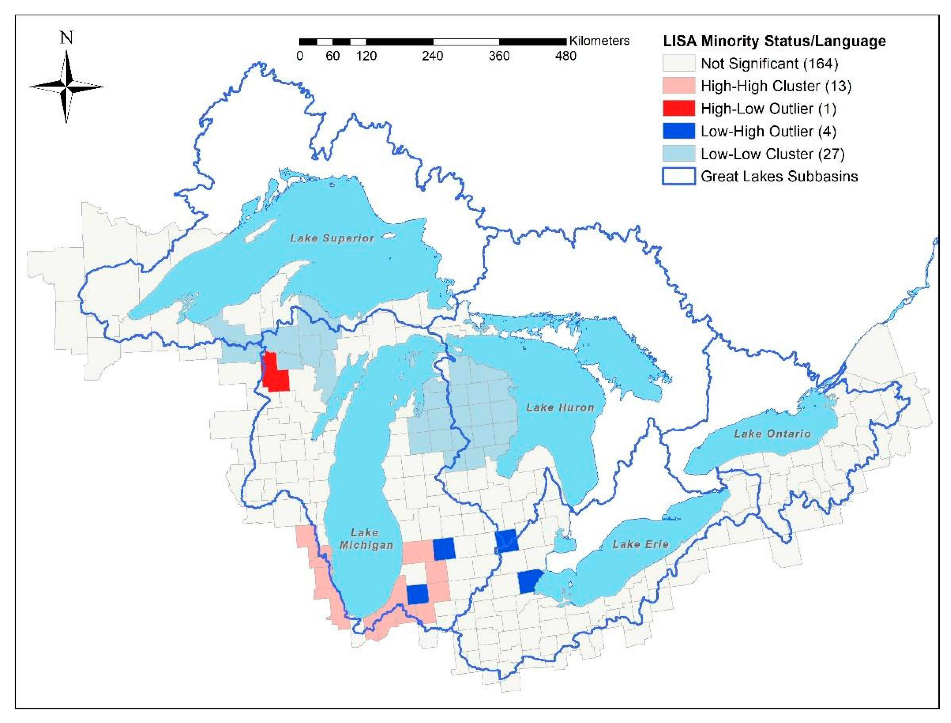
3.3. Minority Status and Language
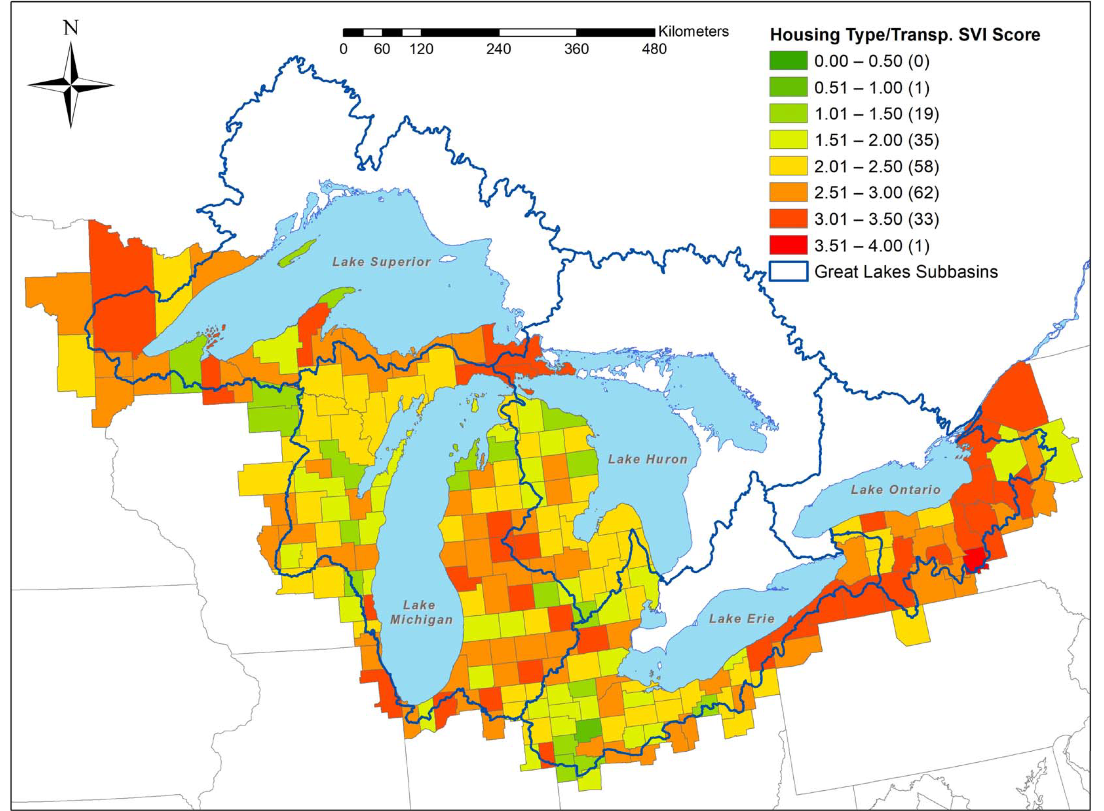
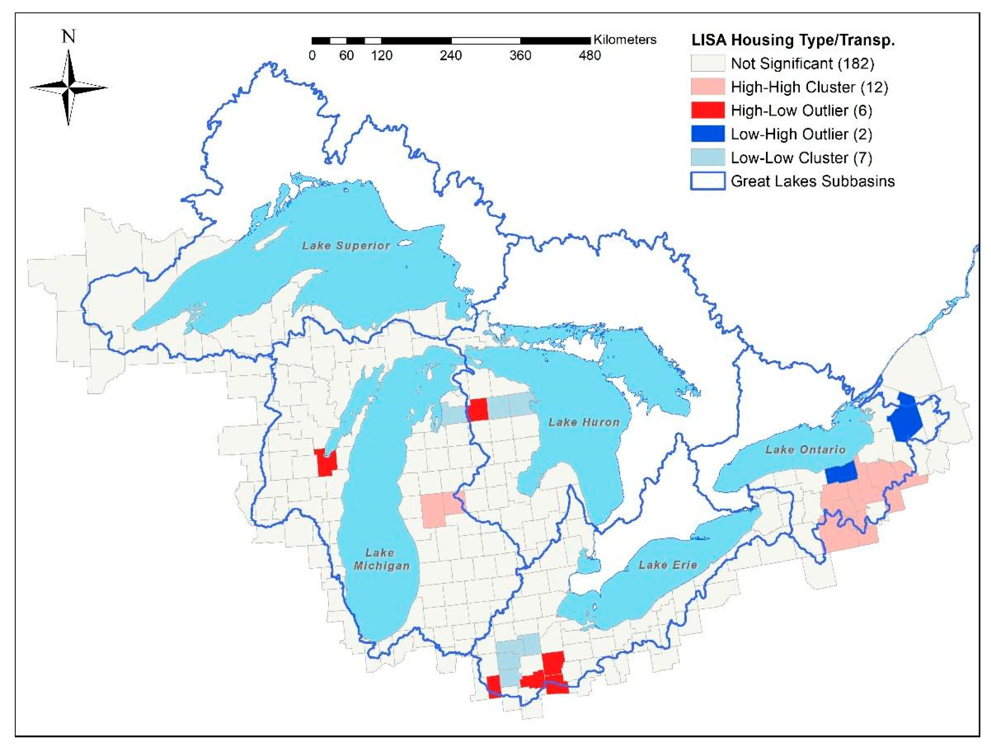
3.4. Housing Type and Transportation
3.5. Social Vulnerability by Region
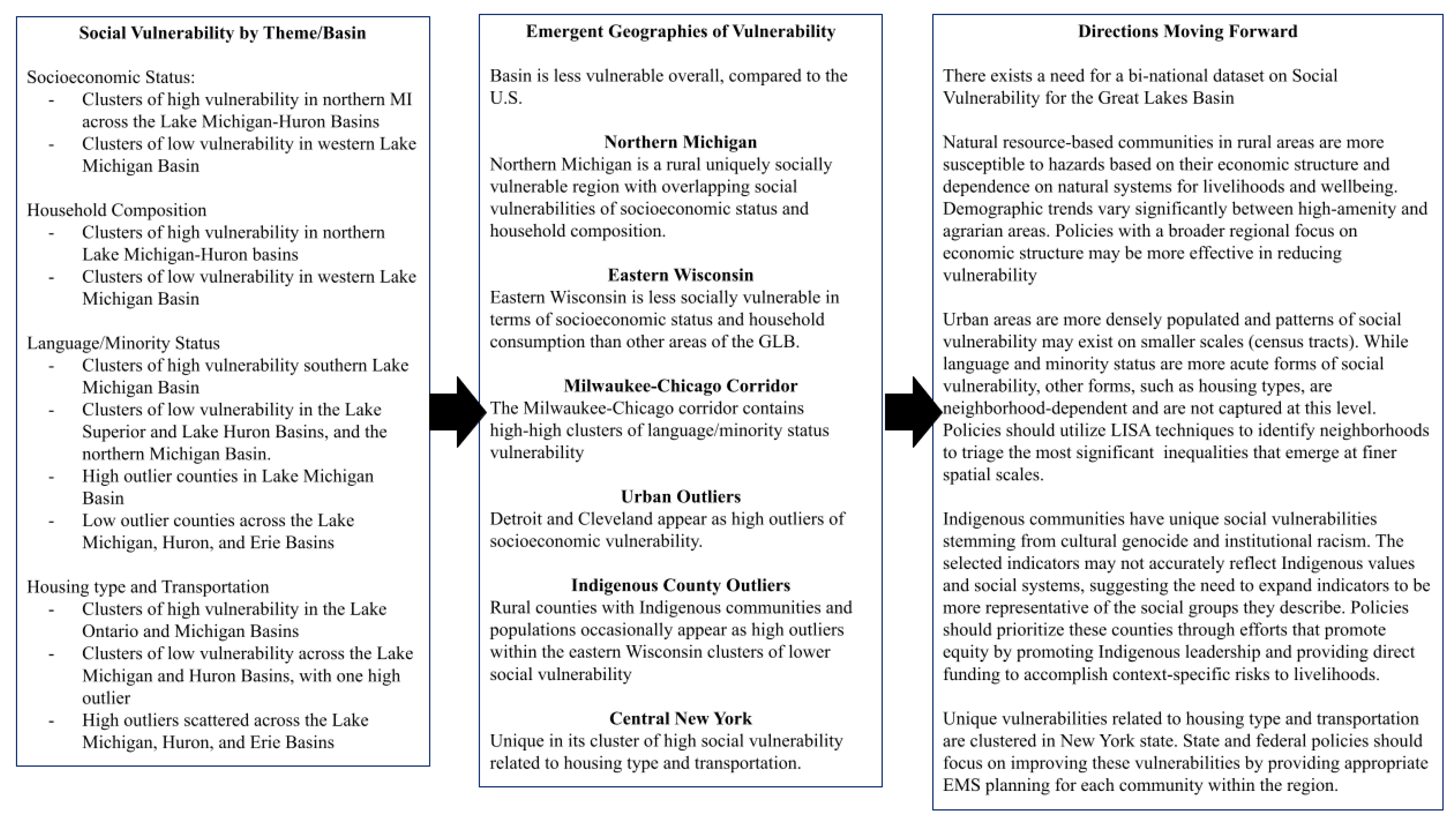
4. Discussion
Limitations
5. Conclusions
Author Contributions
Funding
Data Availability Statement
Conflicts of Interest
References
- Méthot, J.; Huang, X.; Grover, H. Demographics and societal values as driver of change in the Great Lakes-St. Lawrence River basin. J. Great Lakes Res. 2015, 41, 30–44. [Google Scholar] [CrossRef]
- Laurent, K.L.; Friedman, K.B.; Krantzberg, G.; Scavia, D.; Creed, I.F. Scenario analysis: An integrative and effective method for bridging disciplines and achieving a thriving Great Lakes-St. Lawrence River basin. J. Great Lakes Res. 2015, 41, 12–19. [Google Scholar] [CrossRef]
- Bartolai, A.M.; He, L.; Hurst, A.E.; Mortsch, L.; Paehlke, R.; Scavia, D. Climate change as a driver of change in the Great Lakes St. Lawrence River Basin. J. Great Lakes Res. 2015, 41, 45–58. [Google Scholar] [CrossRef]
- Centers for Disease Control and Prevention’s (CDC) Social Vulnerability Index (SVI). Agency for Toxic Substances and Disease Registry. Geospatial Research, Analysis, and Services Program. Database U.S. 2018. Available online: https://www.atsdr.cdc.gov/placeandhealth/svi/data_documentation_download.html (accessed on 13 May 2021).
- Colburn, L.L.; Jepson, M.; Weng, C.; Sears, T.; Weiss, J.; Hare, J.A. Indicators of climate change and social vulnerability in fishing dependent communities along the Eastern and Gulf Coasts of the United States. Mar. Policy 2016, 74, 323–333. [Google Scholar] [CrossRef]
- Wood, N.J.; Burton, C.G.; Cutter, S.L. Community variations in social vulnerability to Cascadia-related tsunamis in the U.S. Pacific Northwest. Nat. Hazards 2010, 52, 369–389. [Google Scholar] [CrossRef] [Green Version]
- Morrow, B.H. Identifying and mapping community vulnerability. Disasters 1999, 23, 1–18. [Google Scholar] [CrossRef]
- Rifat, S.A.A.; Liu, W. Measuring community disaster resilience in the conterminous coastal United States. ISPRS Int. J. Geo-Inf. 2020, 9, 469. [Google Scholar] [CrossRef]
- Flanagan, B.E.; Hallisey, J.E.; Adams, E.; Lavery, A. Measuring community vulnerability to natural and anthropogenic hazards: The Centers for Disease Control and Prevention’s Social Vulnerability Index. J. Environ. Health 2018, 80, 34–36. Available online: https://www.ncbi.nlm.nih.gov/pmc/articles/PMC7179070/ (accessed on 13 May 2021).
- Adger, W.N. Vulnerability. Glob. Environ. Chang. 2006, 16, 268–281. [Google Scholar] [CrossRef]
- Matarrita-Cascante, D.; Trejos, B.; Qin, H.; Joo, D.; Debner, S. Conceptualizing community resilience: Revisiting conceptual distinctions. Community Dev. J. 2017, 48, 105–123. [Google Scholar] [CrossRef]
- Otto, I.M.; Reckien, D.; Reyer, C.P.O.; Marcus, R.; Le Masson, V.; Jones, L.; Norton, A.; Serdeczny, O. Social vulnerability to climate change: A review of concepts and evidence. Reg. Environ. Chang. 2017, 17, 1651–1662. [Google Scholar] [CrossRef]
- Cutter, S.L.; Boruff, B.J.; Shirley, W.L. Social vulnerability to environmental hazards. Soc. Sci. Q. 2003, 84, 242–261. [Google Scholar] [CrossRef]
- Emrich, C.T.; Cutter, S.L. Social vulnerability to climate-sensitive hazards in the southern United States. Weather Clim. Soc. 2011, 3, 193–208. [Google Scholar] [CrossRef]
- Spielman, S.E.; Tuccillo, J.; Folch, D.C.; Schweikert, A.; Davies, R.; Wood, N.; Tate, E. Evaluating social vulnerability indicators: Criteria and their application to the Social Vulnerability Index. Nat. Hazards 2020, 100, 417–436. [Google Scholar] [CrossRef] [Green Version]
- Tate, E.; Rahman, A.; Emrich, C.T.; Sampson, C.C. Flood exposure and social vulnerability in the United States. Nat. Hazards 2021, 106, 435–457. [Google Scholar] [CrossRef]
- Flanagan, B.E.; Hallisey, E.; Sharpe, J.D.; Merzlufft, C.E.; Grossman, M. On the validity of validation: A commentary on Rufat, Tate, Emrich, and Antolini’s ‘How valid are social vulnerability models’? Ann. Assoc. Am. Geogr. 2021, 111. [Google Scholar] [CrossRef]
- Khajehei, S.; Ahmadalipour, A.; Shao, W.; Mordakhani, H. A place-based assessment of flash flood hazard and vulnerability in the contiguous United States. Sci. Rep. 2020, 10, 448. [Google Scholar] [CrossRef] [Green Version]
- Adger, W.N.; Kelly, P.M. Social vulnerability to climate change and the architecture of entitlements. Mitig. Adapt. Strateg. Glob. Chang. 1999, 4, 253–266. [Google Scholar] [CrossRef]
- Eriksen, C.; Simon, G.L.; Roth, F.; Lakhina, S.J.; Wisner, B.; Adler, C.; Thomalla, F.; Scolobig, A.; Brady, K.; Brundl, M.; et al. Rethinking the interplay between affluence and vulnerability to aid climate change adaptive capacity. Clim. Chang. 2020, 162, 25–39. [Google Scholar] [CrossRef]
- Freudenburg, W.R.; Gramling, R. Natural resources and rural poverty: A closer look. Soc. Nat. Res. 1994, 7, 5–22. [Google Scholar] [CrossRef]
- Peluso, N.L.; Humphrey, C.R.; Fortmann, L.P. The rock, the beach, and the tidal pool: People and poverty in natural resource-dependent areas. Soc. Nat. Res. 1994, 7, 23–38. [Google Scholar] [CrossRef]
- McLellan, S.L.; Hollis, E.J.; Depas, M.M.; Van Dyke, M.; Harris, J.; Scopel, C.O. Distribution and fate of Escherichia coli in Lake Michigan following contamination with urban stormwater and combined sewer overflows. J. Great Lakes Res. 2007, 33, 566–580. [Google Scholar] [CrossRef]
- Patz, J.A.; Vavrus, S.J.; Uejio, C.K.; McLellan, S.L. Climate change and waterborne disease risk in the Great Lakes Region of the U.S. Am. J. Prev. Med. 2008, 35, 451–458. [Google Scholar] [CrossRef] [PubMed]
- Cutter, S.L.; Finch, C. Temporal and spatial challenges in social vulnerability to natural hazards. Proc. Natl. Acad. Sci. USA 2008, 105, 2301–2306. [Google Scholar] [CrossRef] [PubMed] [Green Version]
- Lehnert, E.A.; Wilt, G.; Flanagan, B.; Hallisey, E. Spatial exploration of the CDC’s Social Vulnerability Index and heat-related health outcomes in Georgia. Int. J. Disaster Risk Reduct. 2020, 46, 101517. [Google Scholar] [CrossRef]
- Eriksen, S.H.; Kelly, P.M. Developing credible vulnerability indicators for climate adaptation policy assessment. Mitig. Adapt. Strateg. Glob. Chang. 2006, 12, 495–524. [Google Scholar] [CrossRef]
- De Vet, E.; Eriksen, C.; Booth, K.; French, S. An unmitigated disaster: Shifting from response and recovery to mitigation for an insurable future. Int. J. Disaster Risk Sci. 2019, 10, 179–192. [Google Scholar] [CrossRef] [Green Version]
- IPCC. Climate Change 2007: Impacts, Adaptation and Vulnerability; Contribution of Working Group 2 to the Fourth Assessment Report of the Intergovernmental Panel on Climate Change; Parry, M.L., Canziani, O.F., Palutikof, J.P., van der Linden, P.J., Hanson, C.E., Eds.; Cambridge University Press: Cambridge, UK, 2007; 976p. [Google Scholar]
- Younus, M.A.F.; Kabir, M.A. Climate change vulnerability assessment and adaptation of Bangladesh: Mechanisms, notions and solutions. Sustainability 2018, 10, 4286. [Google Scholar] [CrossRef] [Green Version]
- Flanagan, B.E.; Gregory, E.W.; Hallisey, E.J.; Heitgerd, J.L.; Lewis, B. A social vulnerability index for disaster management. J. Homel. Secur. Emerg. Manag. 2011, 8. Available online: http://www.bepress.com/jhsem/vol8/iss1/3 (accessed on 15 May 2021). [CrossRef]
- Gold, A.; Pendall, R.; Treskon, M. Demographic Change in the Great Lakes Region: Recent Population Trends and Possible Futures; Metropolitan Housing and Communities Policy Center: Washington, DC, USA, 2018. [Google Scholar]
- Gregg, R.M.; Feifel, K.M.; Kershner, J.M.; Hitt, J.I. The State of Climate Change Adaptation in the Great Lakes Region; Ecoadapt: Bainbridge Island, WA, USA, 2012; Available online: https://www7.nau.edu/itep/main/iteps/ORCA/3710_ORCA.pdf (accessed on 15 May 2021).
- Friedman, K.B.; Laurent, K.L.; Kranzberg, G.; Scavia, D.; Creed, I.F. The Great Lakes Futures Project: Principles and policy recommendations for making the lakes great. J. Great Lakes Res. 2015, 41, 171–179. [Google Scholar] [CrossRef]
- Melillo, J.; Yohe, G.W. Climate Change Impacts in the United States: The Third National Climate Assessment; U.S. Global Change Research Program: Washington, DC, USA, 2014. [Google Scholar] [CrossRef]
- Wuebbles, D.; Cardinale, B.; Cherkauer, K.; Davidson-Arnott, R.; Hellmann, J.; Infante, D.; Johnson, L.; de Loe, R.; Lofgren, B.; Packman, A.; et al. An Assessment of the Impacts of Climate Change on the Great Lakes. Environmental Law & Policy Center 2019. Available online: https://cardinale.seas.umich.edu/wp-content/uploads/2020/06/Wuebbles-et-al-Great-Lakes-Climate-Change-Report.pdf (accessed on 13 May 2021).
- Sterner, R.W.; Keeler, B.; Polasky, S.; Poudel, R.; Rhude, K.; Rogers, M. Ecosystem services of Earth’s largest freshwater lakes. Ecosyst. Serv. 2020, 41, 101046. [Google Scholar] [CrossRef]
- Austin, J.A.; Colman, S.M. Lake Superior summer water temperatures are increasing more rapidly than regional air temperatures: A positive ice-albedo feedback. Geophys. Res. Lett. 2007, 34. [Google Scholar] [CrossRef] [Green Version]
- Reinl, K.L.; Sterner, R.W.; Austin, J.A. Seasonality and physical drivers of deep chlorophyll layers in Lake Superior, with implication for a rapidly warming lake. J. Great Lakes Res. 2020, 46, 1615–1624. [Google Scholar] [CrossRef]
- Kraker, D. Duluth Rebuilds Lake Walk to–Hopefully–Withstand Future Storms. MPR News. 2020. Available online: https://www.mprnews.org/story/2020/12/21/duluth-rebuilds-lakewalk-to-hopefully-withstand-future-storms (accessed on 14 May 2021).
- Lake Superior Lake Wide Action and Management Plans (LAMP). 2019. Available online: https://binational.net/wp-content/uploads/2021/03/FINAL-English-Lake-Superior-2019-Annual-Report.pdf (accessed on 15 May 2021).
- Lake Michigan Lake Wide Action and Management Plans (LAMP). 2018. Available online: https://binational.net/wp-content/uploads/2019/03/LM_LAMP_AR_2018_final.pdf (accessed on 15 May 2021).
- Great Lakes Surf Rescue Project. Statistics. Available online: https://glsrp.org/statistics/ (accessed on 13 May 2021).
- Associated Press. High Water Wreaks Havoc on Great Lakes, Swamping Communities. AP News; 7 February 2020. Available online: https://apnews.com/article/lake-michigan-in-state-wire-manistee-mi-state-wire-erosion-cdd234381027aa31138767bd3d935ef7 (accessed on 15 May 2021).
- Olson, K.R.; Miller, G.A. St. Lawrence Seaway: Western Great Lakes Basin. J. Water Resour. Prot. 2020, 12, 637–656. Available online: https://www.scirp.org/journal/jwarp (accessed on 15 May 2021). [CrossRef]
- Lake Huron Lake Wide Action and Management Plans (LAMP). 2019. Available online: https://binational.net/wp-content/uploads/2021/03/English-Lake-Huron-2019-Annual-Report.Mar_.9.2021.pdf (accessed on 15 May 2021).
- Michigan Dept. of Environment, Great Lakes, and Energy. Great Lakes Map. 2019. Available online: https://www.michigan.gov/egle/0,9429,7-135-3313_3677-15926--,00.html (accessed on 15 May 2021).
- Lake Erie Lake Wide Action and Management Plans. 2019. Available online: https://binational.net/2021/03/22/lear2019/ (accessed on 15 May 2021).
- Lake Ontario Lake Wide Action and Management Plans. 2019. Available online: https://binational.net/wp-content/uploads/2021/03/FINAL-English-Lake-Ontario-2019-Annual-Report.pdf (accessed on 15 May 2021).
- New York State Official Website. Governor Cuomo Directs New York State Department of Environmental Conservation to Sue the International Joint Commission for Water Level Mismanagement That Devastated Lake Ontario Shoreline Communities. 19 October 2019. Available online: https://www.governor.ny.gov/news/governor-cuomo-directs-new-york-state-department-environmental-conservation-sue-international (accessed on 15 May 2021).
- U.S. Census Bureau. TIGER/Line Shapefiles. 2020. Available online: https://www.census.gov/cgi-bin/geo/shapefiles/index.php (accessed on 17 May 2021).
- USGS GLRI. Great Lakes and Watershed Shapefiles. 2010. Available online: https://www.sciencebase.gov/catalog/item/530f8a0ee4b0e7e46bd300dd (accessed on 17 May 2021).
- Hallegatte, S.; Vogt-Schilb, A.; Rozenberg, J.; Bangalore, M.; Beaudet, C. From poverty to disaster and back: A review of the literature. Econ. Dis. Clim. Chang. 2020, 4, 223–247. [Google Scholar] [CrossRef] [Green Version]
- Peek, L. Children and disasters: Understanding vulnerability, developing capacities, and promoting resilience—An introduction. Child. Youth Environ. 2008, 18, 1–29. Available online: https://www.jstor.org/stable/10.7721/chilyoutenvi.18.1.0001 (accessed on 15 May 2021).
- McGuire, L.C.; Ford, E.S.; Okoro, C.A. Natural disasters and older US adults with disabilities: Implications for evacuation. Disasters 2007, 31, 49–56. [Google Scholar] [CrossRef] [PubMed]
- Wisner, B.; Blaikie, P.; Cannon, T.; Davis, I. The Challenge of Disasters and our Approach. In At Risk: Natural Hazards, People’s Vulnerability, and Disasters; Wisner, B., Blaike, P., Cannon, T., Davis, I., Eds.; Routledge Press: London, UK, 1994; pp. 3–48. [Google Scholar]
- Thomas, K.; Hardy, R.D.; Lazarus, H.; Mendez, M.; Orlove, B.; Rivera-Collazo, I.; Roberts, J.T.; Rockman, M.; Warner, B.P.; Winthrop, R. Explaining differential vulnerability to climate change: A social science review. Wiley Interdiscip. Rev. Clim. Chang. 2019, 10, e565. [Google Scholar] [CrossRef] [PubMed] [Green Version]
- Pulido, L. Rethinking environmental racism: White privilege and urban development in southern California. Ann. Assoc. Am. Geogr. 2000, 90, 12–40. [Google Scholar] [CrossRef] [Green Version]
- Donner, W.R. The political ecology of disaster: An analysis of factors influencing U.S. tornado fatalities and injuries, 1998–2000. Demography 2007, 44, 669–685. [Google Scholar] [CrossRef] [PubMed]
- Anselin, L. Local indicator of spatial association-LISA. Geogr. Anal. 1995, 27, 93–115. [Google Scholar] [CrossRef]
- Anselin, L. Local spatial autocorrelation (1) LISA and Local Moran. GeoDa Documentation. 2020. Available online: https://geodacenter.github.io/workbook/6a_local_auto/lab6a.html (accessed on 28 April 2021).
- Brooks, M.M. The advantages of comparative LISA techniques in spatial inequality research: Evidence from poverty change in the United States. Spat. Demogr. 2019, 7, 167–193. [Google Scholar] [CrossRef]
- Koks, E.E.; Jongman, B.; Husby, T.G.; Botzen, W.J.W. Combining hazard, exposure and social vulnerability to provide lessons for flood risk management. Environ. Sci. Policy 2015, 47, 42–52. [Google Scholar] [CrossRef]
- Armas, I.; Garvis, A. Social vulnerability assessment using spatial multi-criteria analysis (SEVI model) and the social vulnerability index (SoVi model)—A case study for Bucharest, Romania. Nat. Hazards Earth Syst. Sci. 2013, 13, 1481–1499. [Google Scholar] [CrossRef] [Green Version]
- Frigerio, I.; Carnelli, F.; Cabinio, M.; De Amicis, M. Spatiotemporal pattern of social vulnerability in Italy. Int. J. Disaster Risk Sci. 2018, 9, 249–262. [Google Scholar] [CrossRef] [Green Version]
- ESRI ArcGIS Desktop. How Cluster and Outlier Analysis (Anselin Local Moran’s I) Works. Available online: https://desktop.arcgis.com/en/arcmap/latest/tools/spatial-statistics-toolbox/h-how-cluster-and-outlier-analysis-anselin-local-m.htm (accessed on 29 May 2021).
- USDA Economic Research Service (ERS). County Typology Codes. 2019. Available online: https://www.ers.usda.gov/data-products/county-typology-codes (accessed on 16 May 2021).
- Lujan, C.C. American Indians and Alaska Natives count: The US Census Bureau’s efforts to enumerate the Native population. Am. Indian Q. 2014, 38, 319–341. [Google Scholar] [CrossRef]
- Vickery, J.; Hunter, L.M. Native Americans: Where in environmental justice research? Soc. Nat. Resour. 2016, 29, 36–52. [Google Scholar] [CrossRef] [Green Version]
- Rufat, S.; Tate, E.; Emrich, C.T.; Antolini, F. How valid are social vulnerability models? Ann. Assoc. Am. Geogr. 2019, 109, 1131–1153. [Google Scholar] [CrossRef]
- Krieger, N. A century of census tracts: Health & the body politic (1906–2006). J. Urban Health 2006, 83, 355–361. [Google Scholar] [CrossRef] [Green Version]


| Social Vulnerability Theme | ACS Variables (2014–2018) |
|---|---|
| Socioeconomic Status | % Below Poverty % Unemployed Income per Capita % w/No High School Diploma |
| Household Composition and Disability | % Age 65 or Older % Age 17 or Younger % Civilians w/Disability |
| Minority Status and Language | % Minority % Speaks English “Less than Well” |
| Housing Type and Transportation | % Multi-Unit Structures % Mobile Homes % Crowding % w/No Vehicle Access % Living in Group Quarters |
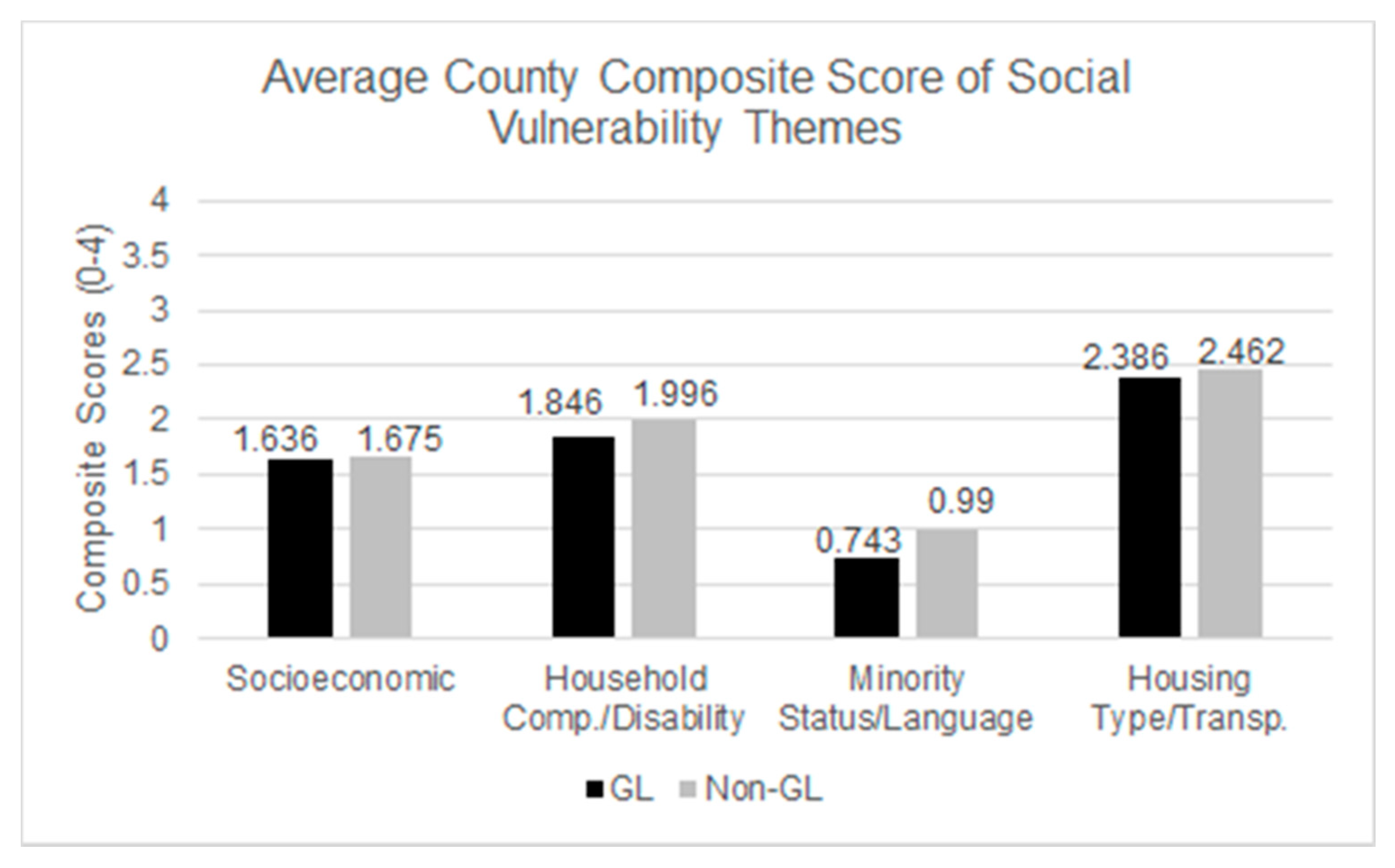
| SVI Theme | GL (209) | Non-GL (2899) | F | Sig. |
|---|---|---|---|---|
| Socioeconomic Status | 1.636 | 1.675 | 0.249 | 0.913 |
| * Household Composition and Disability | 1.846 | 1.996 | 12.008 | <0.001 |
| * Minority Status and Language | 0.743 | 0.99 | 63.994 | <0.001 |
| Housing Type and Transportation | 2.386 | 2.462 | 7.384 | 0.124 |
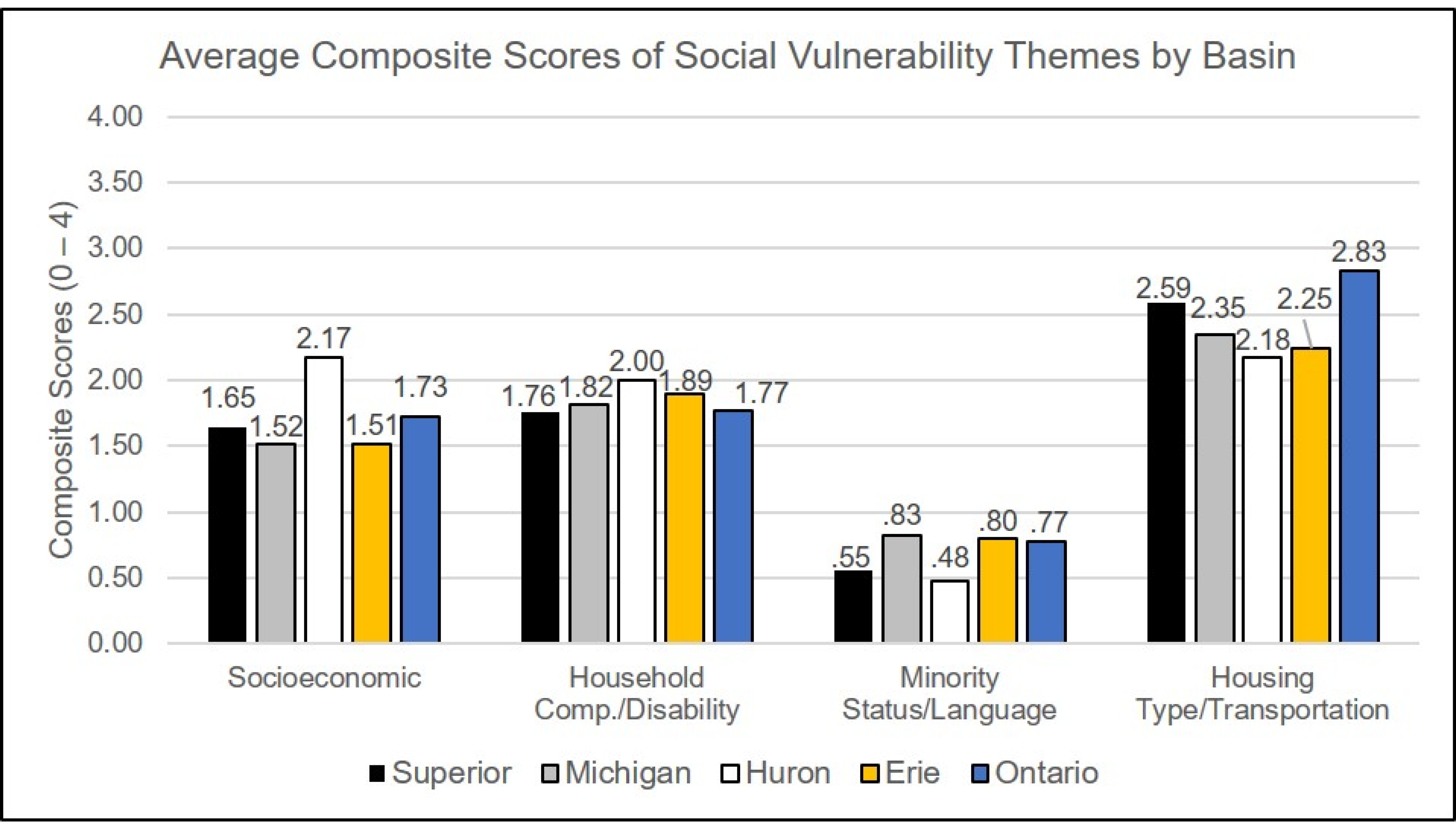
| SVI Theme | Superior | Michigan | Huron | Erie | Ontario | F | Sig. | Diff. * | Sig. |
|---|---|---|---|---|---|---|---|---|---|
| Socioeconomic Status | 1.65 | 1.52 | 2.17 | 1.51 | 1.73 | 5.09 | <0.001 | H ≠ M | <0.001 |
| H ≠ E | <0.001 | ||||||||
| Household Composition and Disability | 1.76 | 1.82 | 2.00 | 1.89 | 1.77 | 1.63 | 0.168 | ns | Ns |
| Minority Status and Language | 0.55 | 0.83 | 0.48 | 0.80 | 0.77 | 6.75 | <0.001 | M ≠ S | 0.017 |
| M ≠ H | <0.001 | ||||||||
| H ≠ E | 0.002 | ||||||||
| H ≠ O | 0.021 | ||||||||
| Housing Type and Transportation | 2.59 | 2.35 | 2.18 | 2.25 | 2.83 | 6.50 | <0.001 | O ≠ M | 0.002 |
| O ≠ H | <0.001 | ||||||||
| O ≠ E | <0.001 |
Publisher’s Note: MDPI stays neutral with regard to jurisdictional claims in published maps and institutional affiliations. |
© 2021 by the authors. Licensee MDPI, Basel, Switzerland. This article is an open access article distributed under the terms and conditions of the Creative Commons Attribution (CC BY) license (https://creativecommons.org/licenses/by/4.0/).
Share and Cite
Fergen, J.T.; Bergstrom, R.D. Social Vulnerability across the Great Lakes Basin: A County-Level Comparative and Spatial Analysis. Sustainability 2021, 13, 7274. https://doi.org/10.3390/su13137274
Fergen JT, Bergstrom RD. Social Vulnerability across the Great Lakes Basin: A County-Level Comparative and Spatial Analysis. Sustainability. 2021; 13(13):7274. https://doi.org/10.3390/su13137274
Chicago/Turabian StyleFergen, Joshua T., and Ryan D. Bergstrom. 2021. "Social Vulnerability across the Great Lakes Basin: A County-Level Comparative and Spatial Analysis" Sustainability 13, no. 13: 7274. https://doi.org/10.3390/su13137274
APA StyleFergen, J. T., & Bergstrom, R. D. (2021). Social Vulnerability across the Great Lakes Basin: A County-Level Comparative and Spatial Analysis. Sustainability, 13(13), 7274. https://doi.org/10.3390/su13137274