Article

The Urbanisation Impacts on the Policy Effects of the Carbon Tax in China

Centre for Environmental Policy, Imperial College London, London SW7 1NE, UK
Sustainability 2021, 13(12), 6749; https://doi.org/10.3390/su13126749
Submission received: 16 May 2021 / Revised: 2 June 2021 / Accepted: 11 June 2021 / Published: 15 June 2021

Abstract

:
In the literature, very few studies have focused on how urbanisation will influence the policy effects of a climate policy even though urbanisation does have profound socioeconomic impacts. This paper has explored the interrelations among the urbanisation, carbon emissions, GDP, and energy consumption in China using the autoregressive distributed lag (ARDL) model. Then, the unit urbanisation impacts are inputted into the policy evaluation framework of the Computable General Equilibrium (CGE) model in 2015–2030. The results show that the urbanisation had a positive impact on the GDP but a negative impact on the carbon emissions in 1980–2014. These impacts were statistically significant, but its impact on the energy consumption was not statistically significant. In 2015–2030, the urbanisation will have negative impacts on the carbon emissions and intensity. It will decrease the GDP and the household welfare under the carbon tax. The urbanisation will increase the average social cost of carbon (ASCC). Hence, the urbanisation will reinforce the policy effects of the carbon tax on the emissions and welfare.

1. Introduction

China has been experiencing rapid urbanisation for decades. The percentage of the urban population increased from 18% in 1978 to 56% in 2015 [1]. The urban population was projected to reach one billion by 2030 [2]. Rapid urbanisation may increase energy consumption because cities are the main contributors to fossil-fuel energy consumption [3]. For example, a one-way positive causal relationship exists from the urbanisation to the energy consumption in China [4]. Conversely, urbanisation could also reduce energy consumption because it saves energy use in transport. For example, the urbanisation was empirically found to reduce the residential energy use in the 12 transition economies [5].
Although a long-term correlation between urbanisation and carbon emissions was already confirmed in the literature [6], urbanisation impacts on carbon emissions are complicated: on the one hand, urbanisation-induced industrialisation results in intensive use of energy, which increases carbon emissions; on the other hand, geographical concentration may enhance energy use efficiency, which decreases carbon emissions. Although previous researchers studied how the Chinese urbanisation affected the historical emissions [7,8,9], the projected urbanisation impacts during the period 2015–2030 remain to be researched in China.
In addition to the environmental impacts, rapid expansion of urban areas could generate profound economic impacts. Urbanisation can generate both positive economic externalities, such as the creation of new jobs and promotion of new technologies, and negative externalities, such as public insecurity and social inequality [10,11].
Hence, urbanisation affects energy consumption, carbon emissions, and economic growth altogether. Studies that partially omit the urbanisation impacts tend to be biased, owing to the omission of an explanatory variable. For example, Zhao and Zhang [3] only focused on the bidirectional impacts of the urbanisation on the energy consumption in China during the years 1980–2010. As Zhao and Zhang [3] excluded the direct urbanisation impacts on the emissions, their results might be biased, owing to the fact that the urbanisation could affect the emissions directly [12]. In contrast, Al-mulali, Sab [13] and Wang, Fang [4] neglected the urbanisation impacts on the economic growth. With the omission of an influential explanatory variable, these studies may not give full understanding of the urbanisation impacts. In comparison to the results in Zhang, Yi et al. [14] could be much more trustworthy, as they fully studied the relation between the urbanisation and its three influential factors.
The complicated socioeconomic impacts of the urbanisation are likely to change the policy effects of the Chinese climate policies. Nevertheless, very few previous studies have modelled urbanisation impacts on the policy effects. Neglecting the urbanisation impacts is likely to cause a misunderstanding regarding climate policies because the structural transition in urban population has a significant influence on efforts to mitigate carbon emissions [15]. Therefore, it is important that the urbanisation impacts should be modelled in the evaluation of climate policies. In the policy evaluation framework, the social cost of carbon (SCC) is usually used to denote whether a climate policy can cost-effectively abate carbon emissions. In other words, the SCC stands for the costs of the emissions of an additional tonne of carbon dioxide [16], and thus it is used to denote the marginal welfare impact of the emissions [17].
This paper contributes to the literature by incorporating the urbanisation impacts in the evaluation framework of the climate policy. Specifically, I have used an ARDL model to study the historical urbanisation impacts during the period 1980–2014 in China. I assume that the historical ARDL interrelations will remain unchanged in 2015–2030. Based on the projected urbanisation data given by UN [18], the projected urbanisation impacts are inputted into the Computable General Equilibrium (CGE) model for the policy evaluation.

2. Data

The coefficients of the ARDL model are calculated using the historical data. The Chinese carbon emission and GDP data are from the World Development Indicators (WDI) by World Bank [19]. The Chinese energy consumption data are from China Energy Statistical Yearbook by NBS [20]. The historical and projected Chinese urbanisation data are from the 2018 World Urbanisation Prospects (WUP) by the United Nations [18].

3. Method

An ARDL model provides reliable results when the variables are in the mixed orders of the stationarity [21]; it has become very popular in the literature to analyse the cointegration relations among economic time series. The cointegration relations are identified based on unit root tests. The most commonly used unit root test is an Augmented Dickey-Fuller (ADF) test, also known as the standardized panel unit root test, based on the deviations from the estimated factors [22]. The results of an ADF test were proved to be robust to the different lag specifications and test misspecifications [23], but it was proved to be biased when the selection of lag length is too small or large [24,25]. According to Elliott and Rothenberg [26], a DF-GLS test is preferred when an unknown mean or trend is present. By comparison, proposed by Phillips and Perron [25], a PP test is nonparametric with respect to nuisance parameters, and it is more powerful than an ADF test in finite samples [27]. As the sample size in this paper is small, the results of a PP test could be more reliable than that of an ADF test.
Based on unit root tests, panel cointegration tests provide more reliable results in testing the cointegration presence relative to those obtained by individual tests [28]. The most frequently used panel cointegration test is the Engle–Granger (EG) cointegration test, put forward by Engle and Granger [29]. The EG test was derived from the basic idea that two nonstationary time series are cointegrated if there is a stationary linear combination of them, from which the residuals are also stationary [28].
After the existence of the cointegration relationships is confirmed, an autoregressive distributed lag (ARDL) model is defined according to Pesaran, Shin [30]. Equation (1) shows the long-term ARDL model where the carbon emissions are the dependent variable. Similar equations can be written when the energy consumption or GDP is the dependent variable. As this paper is targeted at the urbanisation impacts, the urbanisation rate is only introduced as an independent variable.
C E t = γ 0 + k = 1 L 1 γ 1 k C E t k + k = 0 L 2 γ 2 k E C t k + k = 0 L 3 γ 3 k U R t k + k = 0 L 4 γ 4 k G D P t k + ε t
In Equation (1), the subscript t refers to the time, namely, a year;   C E t is the carbon emissions. E C t k , U R t k , and G D P t k stand for the energy consumption, urbanisation rate, and GDP in Year t k , respectively. L 1   ,   L 2   ,   L 3   ,   L 4 are the optimal lagged orders selected by the Schwarz Information Criterion (SIC). The study period of this paper is 2015–2030, which complies with the predictive study in Sun, Zhou [31]. ε t is the residual term; presumably, it is a white noise showing the independence and equal variance. γ 0 ,   γ 1 k ,   γ 2 k ,   γ 3 k ,   γ 4 k are the regression coefficients, and γ 0 is the intercept. As the variables are taken into their logarithm forms, the coefficients denote the elasticities.
To check the robustness of the ARDL model, I have performed the diagnostic tests to test the existence of the heteroskedasticity, autocorrelation, and multicollinearity. I have also used a histogram to check whether the normality assumption is violated and a recursive residual plot to check whether the model is stable.
Once the historical unit impacts are captured by the ARDL model, I input the urbanisation impacts into the policy evaluation framework, assuming that the historical ARDL relationship in 1980–2014 will remain unchanged in 2015–2030. The urbanisation impacts on the carbon emissions and GDP are also assumed to be equal across the sectors and households. This is because in the CGE model, a presentative household and enterprise are introduced to denote the economic behaviours of the entire sectors and households, respectively.
{ C E i t u r = C E i t ( 1 + u r t C E ) S G D P i t u r = S G D P i t ( 1 + u r t G D P ) E C i t u r = E C i t ( 1 + u r t E C )
In Equation (2), E i t u r , S G D P i t u r , and E C i t u r refer to the revised carbon emissions, sectoral GDP, and energy consumption when the net urbanisation impacts are considered. u r t C E , u r t G D P , and u r t E C stand for the unit urbanisation impact on the carbon emissions, GDP, and energy consumption, respectively.
Then, the unit urbanisation impacts are inputted into the Computable General Equilibrium (CGE) model for the policy evaluation. Stemming from the general equilibrium theory of Walras, CGE models have been widely used in policy simulations or evaluations [32,33,34]. In this paper, the CGE model has two regions (China and the rest of the world) and four economic entities (the representative household, enterprise, foreigner, and government). The social accounting matrix (SAM) of the CGE model is based on the 2015 China Input–Output (IO) Table. There are 42 sectors in the 2015 IO Table, but only 29 sectors are left through the sector aggregation and disaggregation, according to Guo, Zhang [35]. The CGE model consists of five blocks:

3.1. Production Block

In the production block, the top production function is formed by a Leontief function. The other levels of the production functions are formed by constant elasticity of substitution (CES) functions. In the CES functions, the elasticity parameters are from Guo, Zhang [35]. A sensitivity analysis is conducted to analyse how sensitive the model results are to the elasticity parameters.

3.2. Income–Expenditure Block

In this block, the representative household consumes either the domestic or foreign goods, whilst its income source is the labour, capital, and money transfers. In contrast, the income of the representative enterprise only comes from the capital, but its expenditure includes the tax and money transfers. The income of the representative government comes from the taxes, and its expenditure includes the consumption, money transfers, and savings.

3.3. Trade Block

In this block, the trade function is based on the Armington [36] assumption that goods produced in different regions are imperfect substitutes. Profit maximisation drives the representative enterprise or foreigner to sell its goods either in the domestic or foreign market.

3.4. Dynamic Block

In this paper, the exogenously determined dynamic variables are the population, price, energy consumption growth rate, and output growth rate. The projected Chinese population will follow the medium variant scenario in 2017 World Population Prospects (WPP) by UN [37]. The projected price change is based on OECD [38]. The projected energy consumption growth rate is from the reference scenario in 2017 International Energy Outlook by EIA [39]. The output growth of the energy sectors will follow the projected growth of the energy consumption, whilst the output growth of the nonenergy sectors will follow the regional GDP long-term forecast by OECD [40].

3.5. Model Closure

In this block, the market clearance is applied, which means no free disposability. The zero profit is also applied, which implies constancy of returns to scale in production and perfectly competitive markets for produced commodities [41]. Thirdly, the income balance denotes that all the entities exhaust their incomes, but deficits are not allowed.
Finally, a sensitivity test is performed to analyse how robust the model results are to the given elasticity parameters. In this paper, all the elasticity parameters will change by ±10%, ±20%, and ±50%, because in the range of ±50%, the inputs in some sectors may turn from poor (good) substitutes to good (poor) substitutes [42]. Generally, the low elasticity parameters imply that the economy is flexible, while the high elasticities imply that the economy is stringent.

4. Results

Tables S1 and S2 in Supplementary Materials show the results of the unit root tests. The first-order difference of C E t does not have a unit root according to the PP test, but the ADF and DF-GLS tests show an opposite result. I conservatively believe that C E t is integrated for order two as both tests show that the second-order difference is stationary. Similarly, Tables S1 and S2 imply that G D P t is integrated for order one, whilst E C t and U R t are integrated for order two.
Table 1 presents the EG test results. When 2 C E t is the dependent variable, the Tau-Statistic and Z-Statistic are both statistically significant, implying that the EG test confirms the existence of a cointegration relationship. Similarly, the EG test also confirms the existence of a cointegration relationship when 2 E C t and G D P t are the dependent variable. As three cointegration relationships are confirmed by the EG test, three ARDL models are constructed correspondingly, and the results are shown in Table 2. In the ARDL models, the inclusion of the constant or trend is based on the information criteria to select the model that fits the data best.
Table 2 displays the coefficients and their significance levels in the ARDL models. If 2 C E t is the dependent variable, the urbanisation has a positive impact on it. The coefficient of 2 U R t is statistically significant at the 1% level, and it means that when 2 U R t increases (decreases) by 1%, 2 E t will increase (decrease) by 3.51%. When 2 E C t is the dependent variable, the coefficient of 2 U R t is not statistically significant, implying that the urbanisation does not have a statistically significant impact on the energy consumption. When Δ G D P t is the dependent variable, the coefficient of U R t is statistically significant.
In Supplementary Materials, Tables S3 and S4 display the results of the robust tests. Table S3 implies that the null hypotheses of the residual equal variances are accepted; the LM test’s null hypotheses that the residuals do not have serial correlations are accepted. Table S4 implies that there are no severe multicollinearity problems in the 2 C E t and 2 E C t model. However, in the Δ G D P t model, the multicollinearity can be a serious problem. Although the multicollinearity may inflate the variations of the coefficients, the estimated coefficients are still unbiased. As the coefficient of Δ U R t is statistically significant, I conclude that the multicollinearity has not generated severe adverse consequences on the study of the urbanisation impacts on the GDP.
Table S5 in Supplementary Materials shows the results of the normality test for the regression residuals. According to Table S5, the p-values of the Jarque–Bera tests are statistically insignificant, implying that the null hypotheses that the residuals are normally distributed are accepted.
Using the projected urbanisation data in 2018 WUP by UN [18], the projected urbanisation impacts on the carbon emissions and GDP are shown in Table 3. The urbanisation will have a consistently negative impact on the carbon emissions. In contrast, the urbanisation will positively affect the GDP, but the impact will attenuate over time.
Figure 1 shows how the projected urbanisation will affect the carbon emissions. According to Figure S1 in Supplementary Materials, the carbon tax will decrease the carbon emissions significantly, compared to the baseline scenario. Hence, the urbanisation impact will strengthen the negative effect of the tax on the emissions.
According to Figure 2, the urbanisation will decrease the carbon intensity, and this impact will decline over time. Figure S2 in Supplementary Materials shows the carbon tax will decrease the carbon intensity. Hence, the urbanisation will reinforce the tax effect on the carbon intensity.
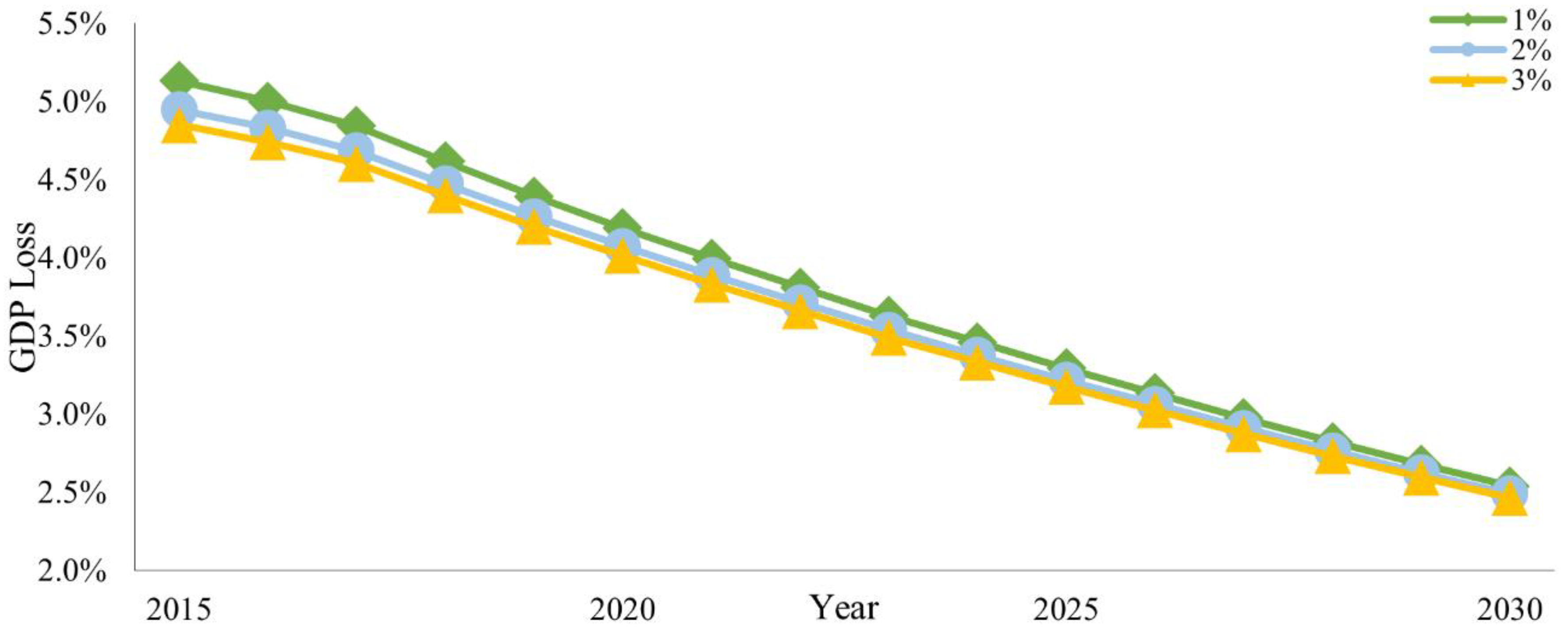
Figure S3 in Supplementary Materials shows that the carbon tax will induce the GDP loss. According to Figure 3, the urbanisation will increase the GDP loss, implying that the urbanisation will strengthen the negative effect of the carbon tax on the GDP. Interestingly, the ARDL model shows that the urbanisation will increase the GDP in the baseline scenario, but the CGE model implies that the urbanisation will decrease the GDP in the tax scenarios.
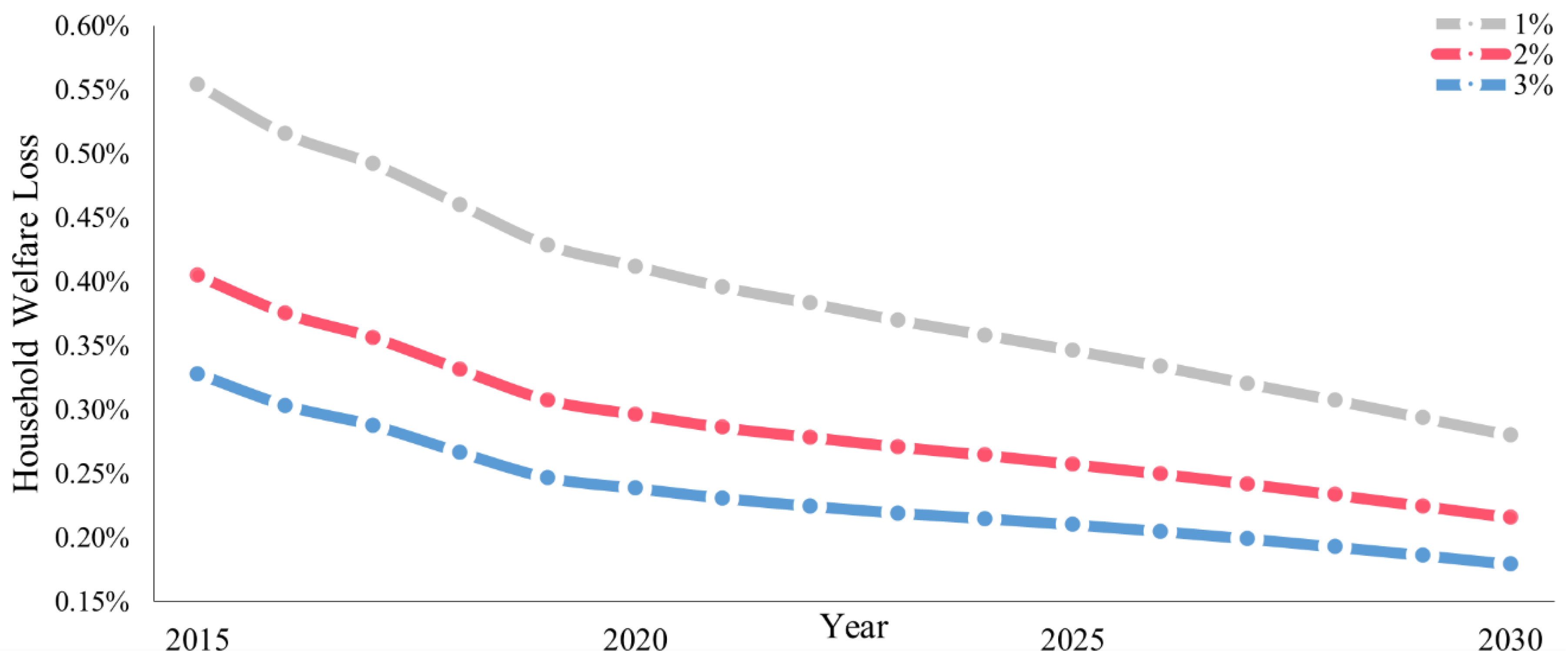
Figure 4 shows how the urbanisation will affect the household welfare loss, induced by the carbon tax shown in Figure S4. According to Figure 4, the urbanisation will increase the welfare loss, implying that the urbanisation will reinforce the negative policy effect of the carbon tax on the household welfare. As the time goes by, this urbanisation impact will gradually decrease.
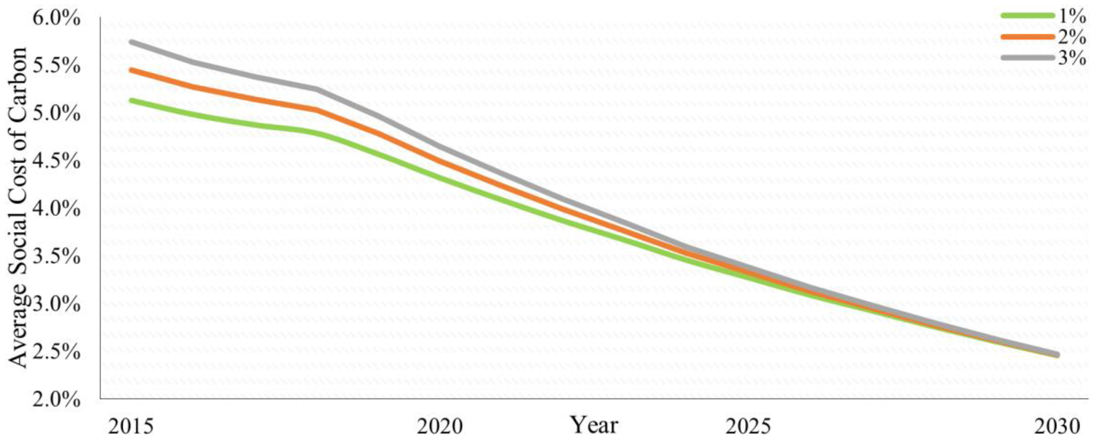
Figure S5 in Supplementary Materials shows the carbon tax will have a complicated effect on the average social cost of carbon (ASCC). This effect became positive in 2019 at the 1% tax, whilst the effect will decline to zero until 2025 at the 2% and 3% tax. Figure 5 shows that the urbanisation will increase the ASCC under the carbon tax. A rise in the tax rate will increase this urbanisation impact, but the influence of the tax rate will diminish over time.
Tables S6 and S7 in Supplementary Materials show the results of the sensitivity analysis. The percentage changes of the model indexes are smaller than the corresponding percentage changes of the elasticity parameters, implying that the model results are robust to the given exogenous values of the elasticity parameters.

5. Discussion

The negative impact of the urbanisation on the carbon emissions analysed in this paper complies with Liu and Liu [43] who argued that, with the development of the urbanisation, its impact on the emissions would become negative. However, Wang and Wu [44] argued that the urbanisation increased the carbon emissions in China. The resulting difference is caused by the adoption of the different methodology: Wang and Wu [44] used the provincial data to study the urbanisation impacts on the energy consumption and carbon emissions, but they omitted the correlation between the urbanisation and economic growth. In contrast, the urbanisation impact is analysed at the country level including the economic factor in this paper. This is because the social accounting matrix (SAM) of the CGE model is based on the China Input–Output, which does not explore the regional details. As China has recently developed the green, circular, and low-carbon economy [45], the omission of the economic factor is likely to result in a biased evaluation of the urbanisation impact.
This paper empirically shows that the urbanisation will decrease the carbon intensity over time. This finding complies with the previous research showing that the urbanisation contributed to the declines in the carbon intensity [46]. The importance of the urbanisation on the carbon intensity reduction in China was also confirmed by Lin and Zhu [47]. Hence, the urbanisation and emission abatement could be harmonious [46].
The urbanisation will promote the GDP growth in the baseline scenario. This finding agrees with Yang and Liu [48] who showed the urbanisation impact on the economic growth was positive for the 266 Chinese cities in 2000–2010. However, in the tax scenarios, the urbanisation will negatively affect the economic growth. Liddle [49] also found that the urbanisation had a “ladder” impact on the income: it had a strong negative impact on the poorest countries, a less negative to neutral impact on the countries with the moderate incomes, and a reinforcing impact on the wealthy countries. As the carbon tax decreases the national income in China [50], the urbanisation impact on the economic growth could become negative if the tax is imposed.
In this paper, the urbanisation will increase the household welfare loss induced by the carbon tax. Analogously, Miao and Wu [2] empirically found that the urbanisation negatively affected the welfare through the lifestyle changes. For example, the populations experiencing the urbanisation would consume more fat and smoke more frequently [51]. By comparison, Chen, Liu [52] showed the health impact of the Chinese urbanisation was complicated, and, particularly, there existed an inverted U-shaped relationship between the health and urbanisation.
The urbanisation will increase the average social cost of carbon (ASCC), which implies that the emission abatement will become costlier under the urbanisation impacts. This finding agrees with the previous research showing that the urbanisation increased the carbon footprint and thus the social cost of carbon in China [53].
In summary, the urbanisation will decrease the emissions and intensity but induce more GDP loss and welfare loss under the carbon tax. Noticeably, all these mentioned urbanisation impacts are quite minimal, which verifies the exogenous introduction of the urbanisation impacts. However, the exogenous introduction may not fully explore the mechanism that the urbanisation influences the policy effects of the carbon tax. This is because the optimal policy is based on the given inputted parameters describing the urbanisation impacts, but these parameters should vary freely to form the optimal policy. Hence, future research may lie in the use of detailed urban–rural population dispersion data to endogenously model the urbanisation as an influential factor of the carbon tax.

6. Conclusions

In 1980–2014, the urbanisation had a positive and statistically significant impact on the GDP. In contrast, it had a negative and statistically significant impact on the carbon emissions in China. This negative impact disagrees with Wang and Wu [44], but it complies with Yao and Kou [46] who argued that the Chinese urbanisation and emission abatement could be harmonious. Noticeably, the urbanisation impact on the energy consumption was not statistically significant. In 2015–2030, the urbanisation will reinforce the negative effects of the carbon tax on the carbon emissions and intensity. The urbanisation will increase the GDP loss and household welfare loss under the carbon tax, implying that the urbanisation will strengthen the negative effects of the tax on the GDP and household welfare. Despite this, the carbon tax will have a complicated effect on the average social cost of carbon (ASCC), and the urbanisation will increase the ASCC. Therefore, I conclude that the urbanisation will strengthen the policy effects of the carbon tax on the emissions and welfare.

Supplementary Materials

The following are available online at https://www.mdpi.com/article/10.3390/su13126749/s1, Figure S1: The Tax Effect on the Carbon Emissions Compared to the Baseline Scenario, Figure S2: The Tax Effect on the Carbon Intensity Compared to the Baseline Scenario, Figure S3: The Policy Effect of the Carbon Tax on the GDP Loss (Unit: 1012 CNY), Figure S4: The Policy Effect of the Carbon Tax on the Household Welfare Loss (Unit: 1012 CNY), Figure S5: The Policy Effect of the Carbon Tax on the ASCC Compared to the Baseline Scenario, Table S1: The Results of the ADF and PP Unit Root Tests, Table S2: The Results of the DF-GLS Unit Root Tests, Table S3: The P-Values of the White and Breusch–Godfrey LM Tests, Table S4: The VIF Scores of the ARDL Models, Table S5: The Results of the Jarque–Bera Normality Tests, Table S6: The Sensitivity Analysis of the Urbanisation Impacts on the 1% Carbon Tax in 2015, Table S7: The Sensitivity Analysis of the Urbanisation Impacts on the 1% Carbon Tax in 2030.

Funding

This research was funded by Imperial College London, grant number OAA0006427 and The APC was funded by Imperial College London.

Informed Consent Statement

Not applicable.

Data Availability Statement

Publicly available datasets were analysed in this study. This data can be found here: https://population.un.org/wup/ (accessed on 1 May 2021); https://databank.worldbank.org/source/world-development-indicators (accessed on 1 May 2021); http://www.stats.gov.cn/tjsj/ndsj/2016/indexeh.htm (accessed on 1 May 2021).

Acknowledgments

The writing of this paper is funded by Imperial College London.

Conflicts of Interest

There are no conflict of interest.

References

  1. NBS. China Statistical Yearbook 2017; China Statistics Press: Beijing, China, 2017. [Google Scholar]
  2. Miao, J.; Wu, X. Urbanization, socioeconomic status and health disparity in China. Health Place 2016, 42, 87–95. [Google Scholar] [CrossRef] [PubMed]
  3. Zhao, P.J.; Zhang, M. The impact of urbanisation on energy consumption: A 30-year review in China. Urban Clim. 2018, 24, 940–953. [Google Scholar] [CrossRef]
  4. Wang, S.; Fang, C.; Guan, X.; Pang, B.; Ma, H. Urbanisation, energy consumption, and carbon dioxide emissions in China: A panel data analysis of China’s provinces. Appl. Energy 2014, 136, 738–749. [Google Scholar] [CrossRef]
  5. Pablo-Romero, M.D.; Sánchez-Braza, A.; Anna, G. Relationship between economic growth and residential energy use in transition economies. Clim. Dev. 2018, 11, 338–354. [Google Scholar] [CrossRef]
  6. Pata, U.K. The effect of urbanization and industrialization on carbon emissions in Turkey: Evidence from ARDL bounds testing procedure. Environ. Sci. Pollut. Res. 2017, 25, 7740–7747. [Google Scholar] [CrossRef]
  7. Zhao, H.; Chen, Y.M. Research on relationship between urbanization process and carbon emission reduction in China. China Soft Sci. 2013, 3, 184–192. [Google Scholar]
  8. Ji, S.D.; Wu, H.; Wang, Z. Openness to trade, urbanization and carbon dioxide emissions-based on panel data of China’s urban bound co-integration analysis. Econ. Probl. 2013, 12, 31–35. [Google Scholar]
  9. Dong, X.Y.; Yuan, G.Q. China’s Greenhouse Gas emissions’ dynamic effects in the process of its urbanization: A perspective from shocks decomposition under long-term constraints. In Proceedings of the 2010 International Conference on Energy, Environment and Development (Iceed2010), Kuala Lumpur, Malaysia, 8–9 December 2011; Volume 5, pp. 1660–1665. [Google Scholar]
  10. Dociu, M.; Dunarintu, A. The Socio-Economic Impact of Urbanization. Int. J. Acad. Res. Account. Financ. Manag. Sci. 2012, 2, 47–52. [Google Scholar]
  11. Deng, X.; Huang, J.; Rozelle, S.; Zhang, J.; Li, Z. Impact of urbanization on cultivated land changes in China. Land Use Policy 2015, 45, 1–7. [Google Scholar] [CrossRef]
  12. Xu, Q.; Dong, Y.-X.; Yang, R. Urbanization impact on carbon emissions in the Pearl River Delta region: Kuznets curve relationships. J. Clean. Prod. 2018, 180, 514–523. [Google Scholar] [CrossRef]
  13. Al-Mulali, U.; Sab, C.N.B.C.; Fereidouni, H.G. Exploring the bi-directional long run relationship between urbanization, energy consumption, and carbon dioxide emission. Energy 2012, 46, 156–167. [Google Scholar] [CrossRef]
  14. Zhang, Y.-J.; Yi, W.-C.; Li, B.-W. The Impact of Urbanization on Carbon Emission: Empirical Evidence in Beijing. Energy Procedia 2015, 75, 2963–2968. [Google Scholar] [CrossRef] [Green Version]
  15. Wang, J.; Wu, Y.; Zhao, Y.; He, S.; Dong, Z.; Bo, W. The population structural transition effect on rising per capita CO2 emissions: Evidence from China. Clim. Policy 2019, 19, 1250–1269. [Google Scholar] [CrossRef]
  16. Fleurbaey, M.; Ferranna, M.; Budolfson, M.; Dennig, F.; Mintz-Woo, K.; Socolow, R.; Spears, D.; Zuber, S. The Social Cost of Carbon: Valuing Inequality, Risk, and Population for Climate Policy. Monist 2018, 102, 84–109. [Google Scholar] [CrossRef]
  17. Nordhaus, W.D. Revisiting the social cost of carbon. Proc. Natl. Acad. Sci. USA 2017, 114, 1518–1523. [Google Scholar] [CrossRef] [PubMed] [Green Version]
  18. UN. World Urbanization Prospects: The 2018 Revision, Online ed.; UN: New York, NY, USA, 2018. [Google Scholar]
  19. WB. DataBank: World Development Indicators; WB: Washington, DC, USA, 2020. [Google Scholar]
  20. NBS. China Energy Statistical Yearbook 2016; China Statistics Press: Beijing, China, 2016. [Google Scholar]
  21. Kalmaz, D.B.; Kirikkaleli, D. Modeling CO2 emissions in an emerging market: Empirical finding from ARDL-based bounds and wavelet coherence approaches. Environ. Sci. Pollut. Res. 2019, 26, 5210–5220. [Google Scholar] [CrossRef]
  22. Pesaran, M.H. A simple panel unit root test in the presence of cross-section dependence. J. Appl. Econ. 2007, 22, 265–312. [Google Scholar] [CrossRef] [Green Version]
  23. Hooker, M.A. Testing for Cointegration—Power Versus Frequency of Observation. Econ. Lett. 1993, 41, 359–362. [Google Scholar] [CrossRef]
  24. Schwert, G.W. Tests for Unit Roots—A Monte-Carlo Investigation. J. Bus. Econ. Stat. 1989, 7, 147–159. [Google Scholar]
  25. Phillips, C.B.; Perron, P. Testing for a Unit-Root in Time-Series Regression. Biometrika 1988, 75, 335–346. [Google Scholar] [CrossRef]
  26. Elliott, G.; Rothenberg, T.J.; Stock, J.H. Efficient Tests for an Autoregressive Unit Root. Economic 1996, 64, 813. [Google Scholar] [CrossRef] [Green Version]
  27. Choi, I.; Chung, B.S. Sampling frequency and the power of tests for a unit root: A simulation study. Econ. Lett. 1995, 49, 131–136. [Google Scholar] [CrossRef]
  28. Mitić, P.; Ivanović, O.M.; Zdravković, A. A Cointegration Analysis of Real GDP and CO2 Emissions in Transitional Countries. Sustainability 2017, 9, 568. [Google Scholar] [CrossRef] [Green Version]
  29. Engle, R.F.; Granger, C.W.J. Co-Integration and Error Correction: Representation, Estimation, and Testing. Econometrica 1987, 55, 251–276. [Google Scholar] [CrossRef]
  30. Pesaran, M.H.; Shin, Y.; Smithc, R.J. Bounds testing approaches to the analysis of level relationships. J. Appl. Econ. 2001, 16, 289–326. [Google Scholar] [CrossRef]
  31. Sun, D.; Zhou, L.; Li, Y.; Liu, H.; Shen, X.; Wang, Z.; Wang, X. New-type urbanization in China: Predicted trends and investment demand for 2015–2030. J. Geogr. Sci. 2017, 27, 943–966. [Google Scholar] [CrossRef]
  32. Li, Z.; Dai, H.; Sun, L.; Xie, Y.; Liu, Z.; Wang, P.; Yabar, H. Exploring the impacts of regional unbalanced carbon tax on CO2 emissions and industrial competitiveness in Liaoning province of China. Energy Policy 2018, 113, 9–19. [Google Scholar] [CrossRef]
  33. Li, W.; Jia, Z. Carbon tax, emission trading, or the mixed policy: Which is the most effective strategy for climate change mitigation in China? Mitig. Adapt. Strat. Glob. Chang. 2017, 22, 973–992. [Google Scholar] [CrossRef]
  34. Guo, Z.; Liu, H. The impact of carbon tax policy on energy consumption and CO2 emission in China. Energy Sources Part B Econ. Plan. Policy 2016, 11, 725–731. [Google Scholar] [CrossRef]
  35. Guo, Z.; Zhang, X.; Zheng, Y.; Rao, R. Exploring the impacts of a carbon tax on the Chinese economy using a CGE model with a detailed disaggregation of energy sectors. Energy Econ. 2014, 45, 455–462. [Google Scholar] [CrossRef]
  36. Armington, S. A theory of demand for products distinguished by place of origin. Staff. Pap. Int. Monet. Fund 1969, 16, 159–178. [Google Scholar] [CrossRef]
  37. UN. World Population Prospects: The 2017 Revision. 2017. Available online: https://www.un.org/development/desa/publications/world-population-prospects-the-2017-revision.html (accessed on 20 March 2019).
  38. OECD. Air and Climate. 2017. Available online: https://stats.oecd.org/ (accessed on 20 October 2019).
  39. EIA. International Energy Outlook 2017. Available online: https://www.eia.gov/outlooks/archive/ieo17/ (accessed on 1 May 2020).
  40. OECD. GDP Long-Term Forecast. 2018. Available online: https://data.oecd.org/gdp/gdp-long-term-forecast.htm (accessed on 1 May 2020).
  41. Sue Wing, I. Computable General Equilibrium Models and Their Use in Economy-Wide Policy Analysis: Everything You Ever Wanted to Know (but Were Afraid to Ask); The MIT Joint Program on the Science and Policy of Global Change: Cambridge, MA, USA, 2004; pp. 1–48. [Google Scholar]
  42. Lu, Y.; Stern, D.I. Substitutability and the Cost of Climate Mitigation Policy. Environ. Resour. Econ. 2015, 64, 81–107. [Google Scholar] [CrossRef]
  43. Liu, F.; Liu, C. Regional disparity, spatial spillover effects of urbanisation and carbon emissions in China. J. Clean. Prod. 2019, 241, 118226. [Google Scholar] [CrossRef]
  44. Wang, Q.; Wu, S.-D.; Zeng, Y.-E.; Wu, B.-W. Exploring the relationship between urbanization, energy consumption, and CO2 emissions in different provinces of China. Renew. Sustain. Energy Rev. 2016, 54, 1563–1579. [Google Scholar] [CrossRef]
  45. He, J.K. Global low-carbon transition and China’s response strategies. Adv. Clim. Chang. Res. 2016, 7, 204–212. [Google Scholar] [CrossRef]
  46. Yao, X.; Kou, D.; Shao, S.; Li, X.; Wang, W.; Zhang, C. Can urbanization process and carbon emission abatement be harmonious? New evidence from China. Environ. Impact Assess. Rev. 2018, 71, 70–83. [Google Scholar] [CrossRef]
  47. Lin, B.; Zhu, J. Energy and carbon intensity in China during the urbanization and industrialization process: A panel VAR approach. J. Clean. Prod. 2017, 168, 780–790. [Google Scholar] [CrossRef]
  48. Yang, Y.; Liu, J.; Zhang, Y. An analysis of the implications of China’s urbanization policy for economic growth and energy consumption. J. Clean. Prod. 2017, 161, 1251–1262. [Google Scholar] [CrossRef]
  49. Liddle, B. The Energy, Economic Growth, Urbanization Nexus across Development: Evidence from Heterogeneous Panel Estimates Robust to Cross-Sectional Dependence. Energy J. 2013, 34, 223–244. [Google Scholar] [CrossRef]
  50. Zhang, X.; Guo, Z.; Zheng, Y.; Zhu, J.; Yang, J. A CGE Analysis of the Impacts of a Carbon Tax on Provincial Economy in China. Emerg. Mark. Financ. Trade 2015, 52, 1372–1384. [Google Scholar] [CrossRef]
  51. Van de Poel, E.; O’Donnell, O.; van Doorslaer, E. Is there a health penalty of China’s rapid urbanization? Health Econ. 2012, 21, 367–385. [Google Scholar] [CrossRef] [PubMed]
  52. Chen, H.; Liu, Y.; Li, Z.; Xue, D. Urbanization, economic development and health: Evidence from China’s labor-force dynamic survey. Int. J. Equity Health 2017, 16, 1–8. [Google Scholar] [CrossRef] [PubMed] [Green Version]
  53. Lee, J.W. Lagged effect of exports, industrialization and urbanization on carbon footprint in Southeast Asia. Int. J. Sustain. Dev. World Ecol. 2019, 26, 398–405. [Google Scholar] [CrossRef]
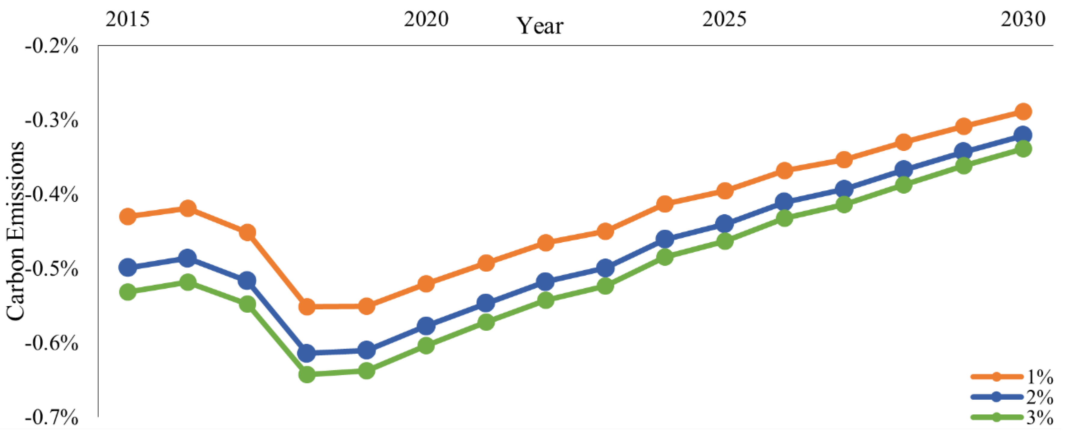
Figure 1. The urbanisation impact on the carbon emissions under the carbon tax. Note: 1%, 2%, and 3% denote the tax rates.
Sustainability 13 06749 g001
Figure 2. The urbanisation impact on the carbon intensity under the carbon tax.
Sustainability 13 06749 g002
Figure 3. The urbanisation impact on the GDP loss under the carbon tax.
Sustainability 13 06749 g003
Figure 4. The urbanisation impact on the household welfare loss under the carbon tax.
Sustainability 13 06749 g004
Figure 5. The urbanisation impact on the ASCC under the carbon tax.
Sustainability 13 06749 g005
Table 1. The results of the EG cointegration tests.
Dependent VariableTau-Statisticp-ValueZ-Statisticp-Value
2 C E t −6.670.0004 **−90.63<0.0001 **
2 E C t −7.54<0.0001 **−41.45<0.0001 **
G D P t −5.020.0035 **−46.74<0.0001 **
Note: and 2 denote the first-order and second-order differences, respectively; ** denotes statistical significance at the 5% level.
Table 2. The results of the ARDL models.
Dependent VariableIndependent VariableCoefficientp-Value
2 C E t 2 C E t 1 −0.43<0.0001 **
2 E C t 1.010.0002 **
2 E C t 1 0.470.0052 **
G D P t 0.180.0772
2 U R t 3.510.0083 **
C −0.0170.1152
2 E C t 2 E C t 1 −0.280.0170 **
2 C E t 0.58<0.0001 **
2 C E t 1 0.350.0110 **
G D P t 0.00310.8946
2 U R t −0.590.6690
Δ G D P t Δ G D P t 1 0.680.0001 **
Δ G D P t 2 −0.370.0342 **
Δ E t 0.250.2804
Δ E C t −0.190.5291
Δ U R t 2.100.0005 **
Note: “C” denotes the constant; ** denotes statistical significance at the 5% level.
Table 3. The projected impacts of urbanisation on the CO2 emissions and GDP.
Year CO2GDPYearCO2GDPYearCO2GDP
2015−0.22%4.75%2021−0.32%3.67%2027−0.25%2.68%
2016−0.21%4.62%2022−0.30%3.49%2028−0.24%2.53%
2017−0.24%4.48%2023−0.30%3.31%2029−0.23%2.40%
2018−0.35%4.27%2024−0.28%3.14%2030−0.21%2.27%
2019−0.35%4.06%2025−0.27%2.98%
2020−0.33%3.86%2026−0.26%2.83%
Publisher’s Note: MDPI stays neutral with regard to jurisdictional claims in published maps and institutional affiliations.