5.2.1. The Influence of Fairness Preference on Revenue Distribution
The initial data of the case is the same as in
Section 4.3.1. Since there’s little difference on the basic data of the three FLSPs, it can be considered that each FLSP has the same status in the overall peer. Therefore,
, takes the same value, 1, for each FLSP
i.
- (1)
Fair-neutral FLSP among members
Situation 1.
Fair-neutral FLSPs account for the majority.
For situation 1, the inequity aversion parameters of the three FLSPs are
and
where FLSP2 and FLSP3 are fair-neutral. The experiments are carried out by changing the value of inequity aversion parameters of FLSP1,
increases from 0 to 0.3, which corresponds to different degrees of FLSP1′ inequity aversion, from fair-neutral to inequity aversion. The results of experiments are shown in
Table 6,
Figure 11 and
Figure 12.
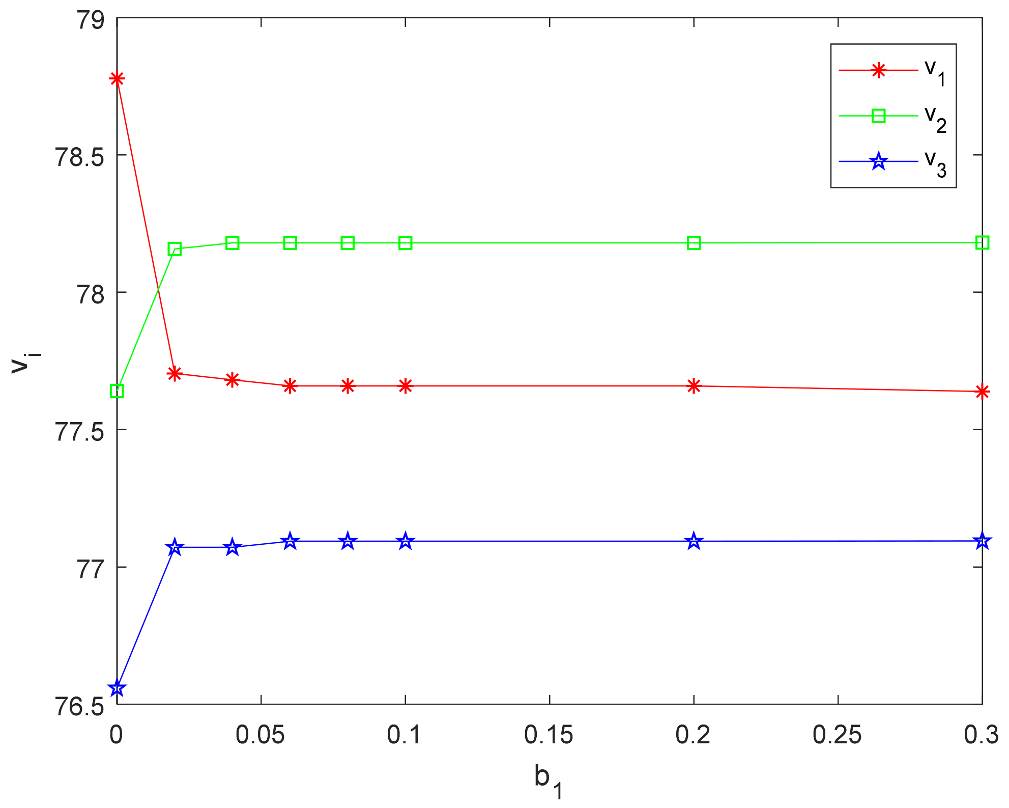
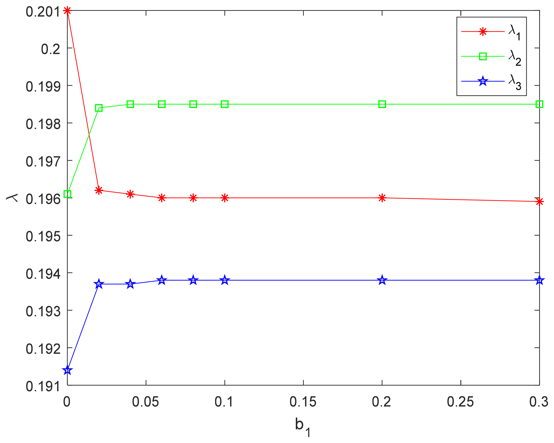
It can be seen from
Table 6 that FLSP1 has the greatest distribution ratio and greatest utility than other FLSPs, when all three FLSPs are fair-neutral. From
Figure 11 and
Figure 12,
and
will decrease, but the ratio of fair-neutral members,
and
will increase when FLSP1 is inequity aversion. The distribution ratio is no longer affected by
when
is the same as the average.
The reasons are as follows: FLSP1 is above average and in an advantageous position while members are fair-neutral. Therefore, negative effects will be generated by advantageous inequity aversion when FLSP1 has inequity aversion. In order to reduce the gap with the average revenue, FLSP1 gives up part of the revenue to other members and reduces the distribution ratio, so that the revenue of the three FLSPs is substantially the same. The negative utility produced by comparison with the average is 0, and the supply chain has the greatest utility.
Compared with situation 1 in
Section 4.3.2, the distribution ratio solved by the original model is too low for members with inequity aversion who seek for greater adverse inequity positive utility, and the fair-neutral member distribution ratio is too high. This is not realistic. With the improved BO model, FLSP1 with inequity aversion only gives up part of its own interests, and the distribution ratio is slightly reduced to make the revenue distribution fairer.
In order to maximize the utility of the supply chain and reduce the inequity aversion negative utility, the of the three FLSPs must be similar, etc., the other three situations should be the same.
What are the impacts on the revenue distribution plan when the three FLSPs value different degrees of their own revenue? The following experiment is carried out for this issue.
B. The inequity aversion parameters of the three FLSPs are
,
, where FLSP2 and FLSP3 are fair-neutral. The parameters of the three FLSPs for their own revenue,
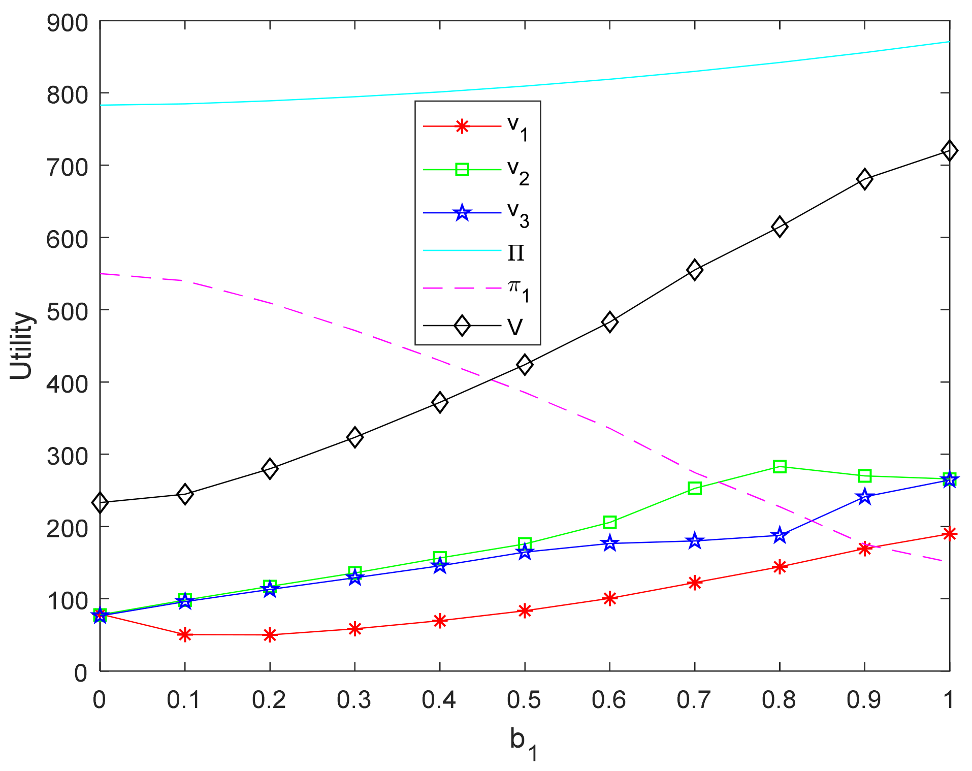
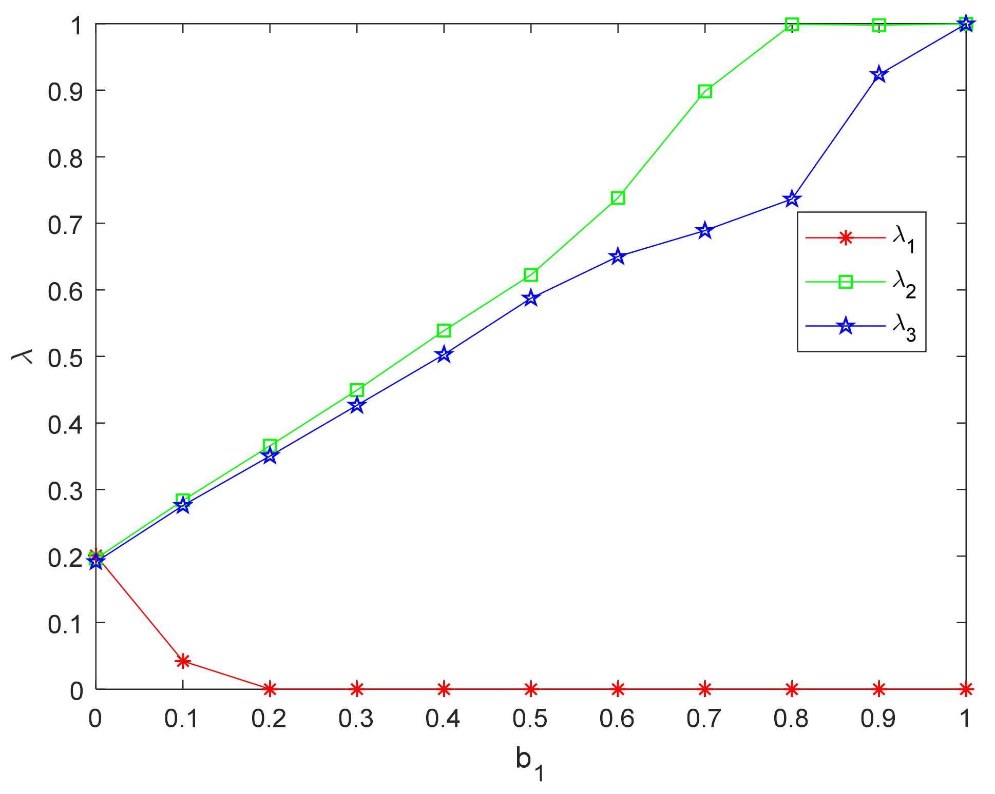
are only to indicate their different attitudes, and they do not have to be too specific. The experiments are carried out by changing the value of inequity aversion parameters of FLSP1,
increases from 0 to 1, which corresponds to different degrees of FLSP1′ inequity aversion, from fair-neutral to extremely inequity aversion. The experimental results are shown in
Table 7 and
Figure 13 and
Figure 14.
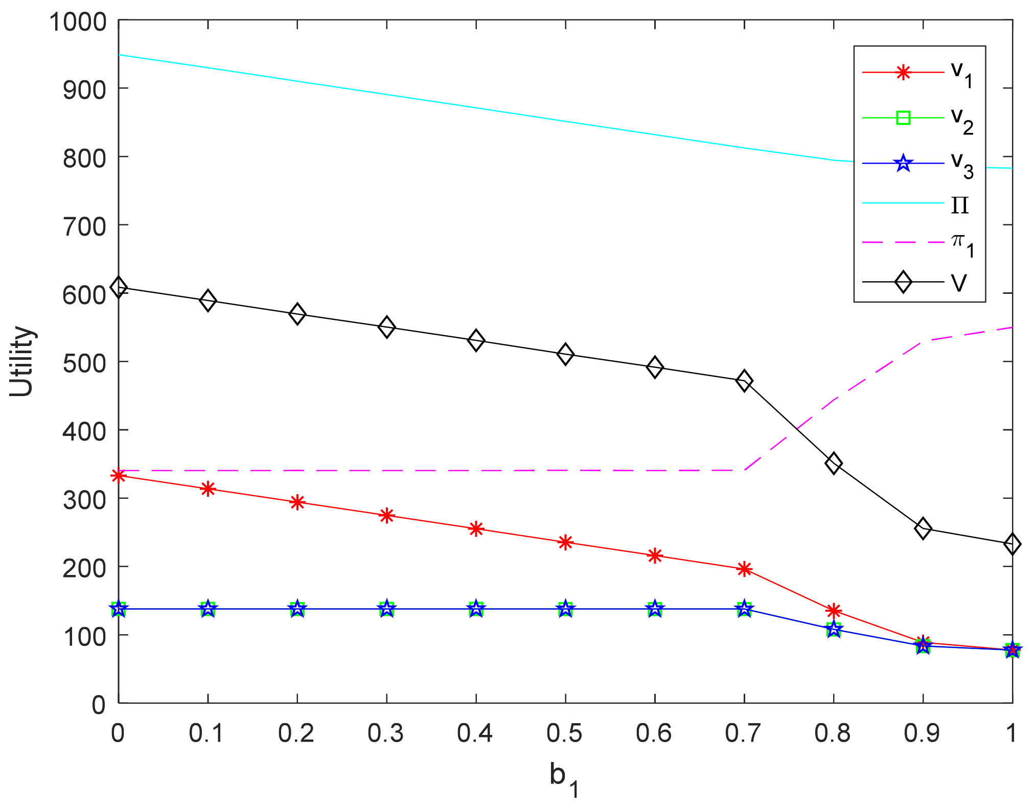
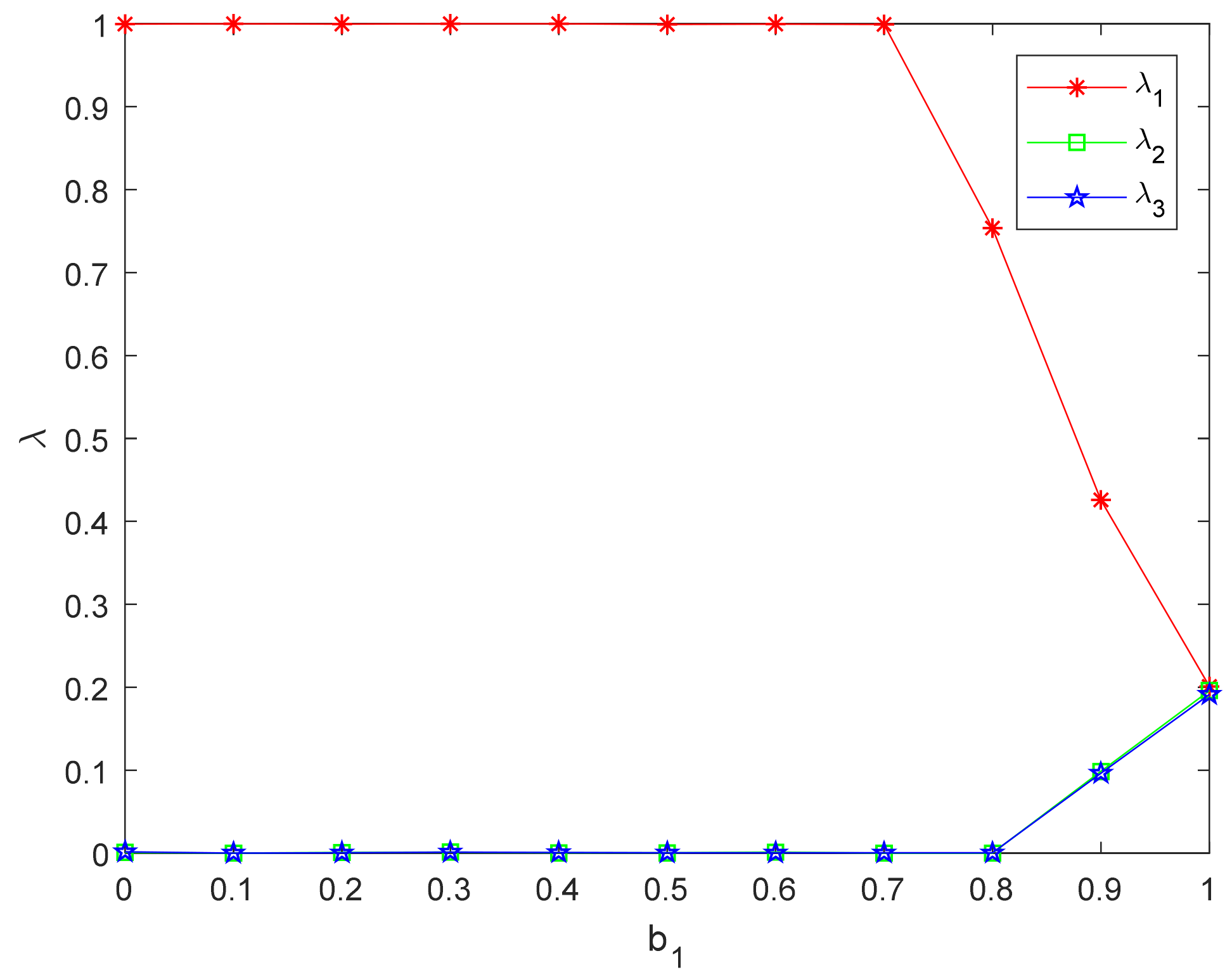
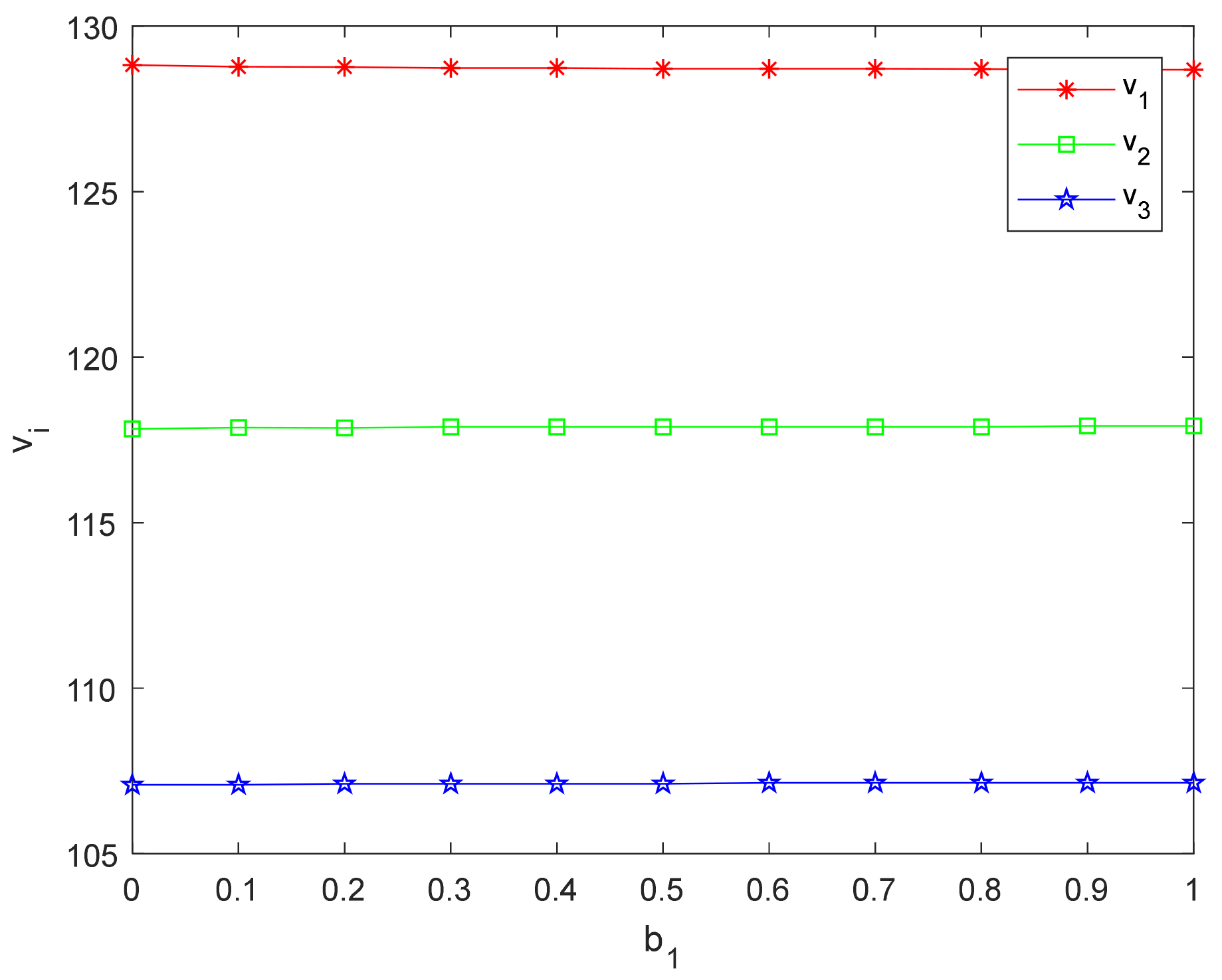
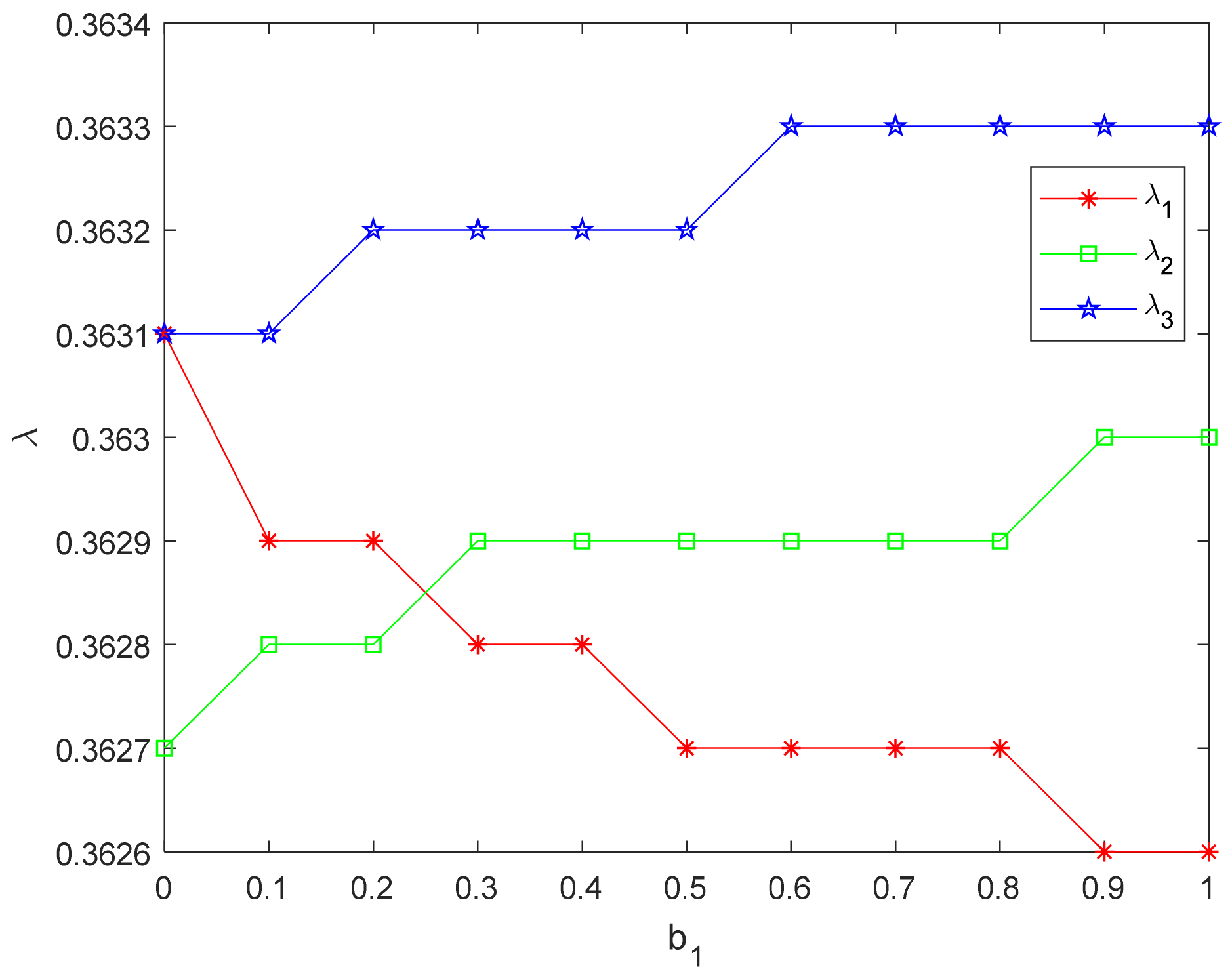
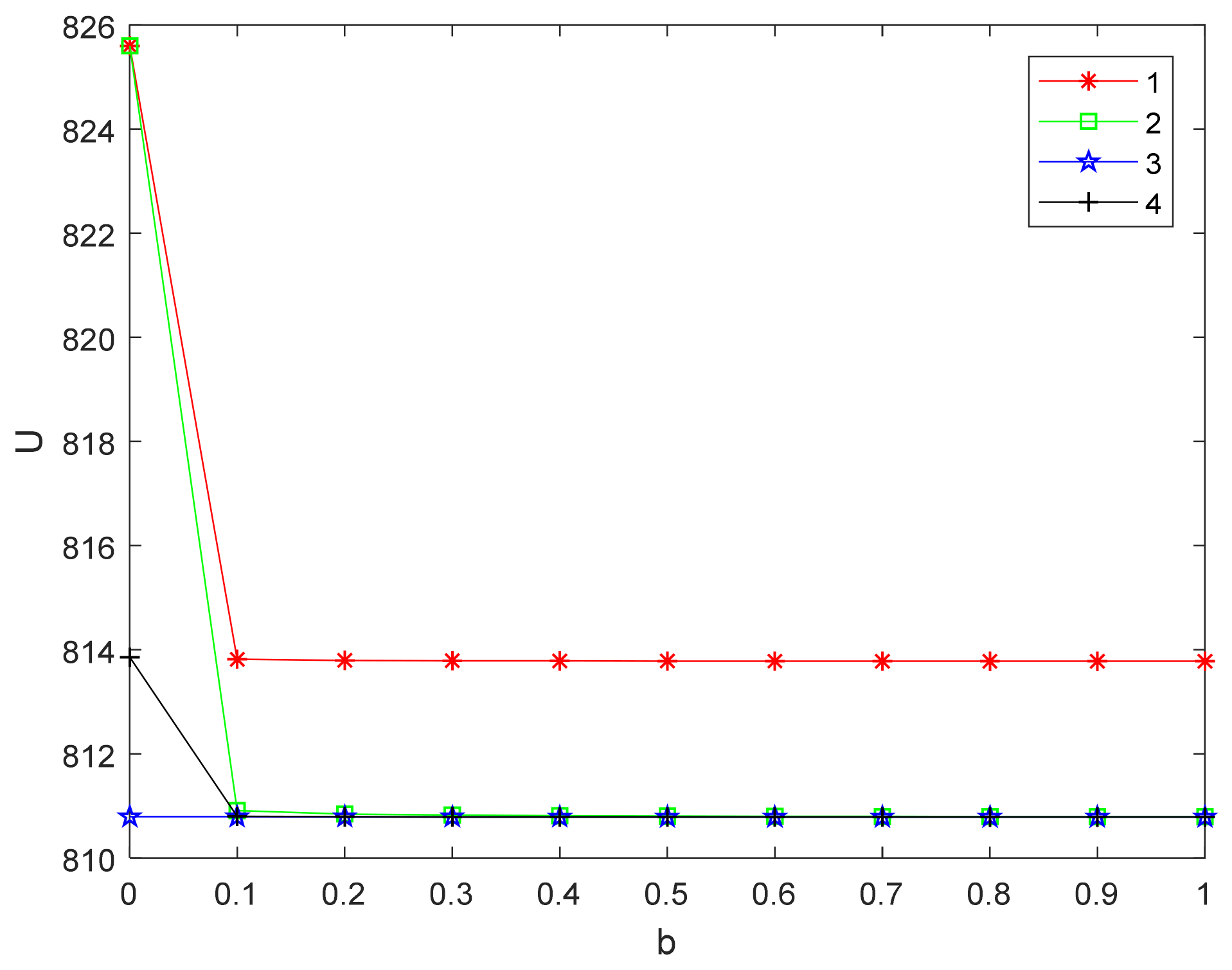
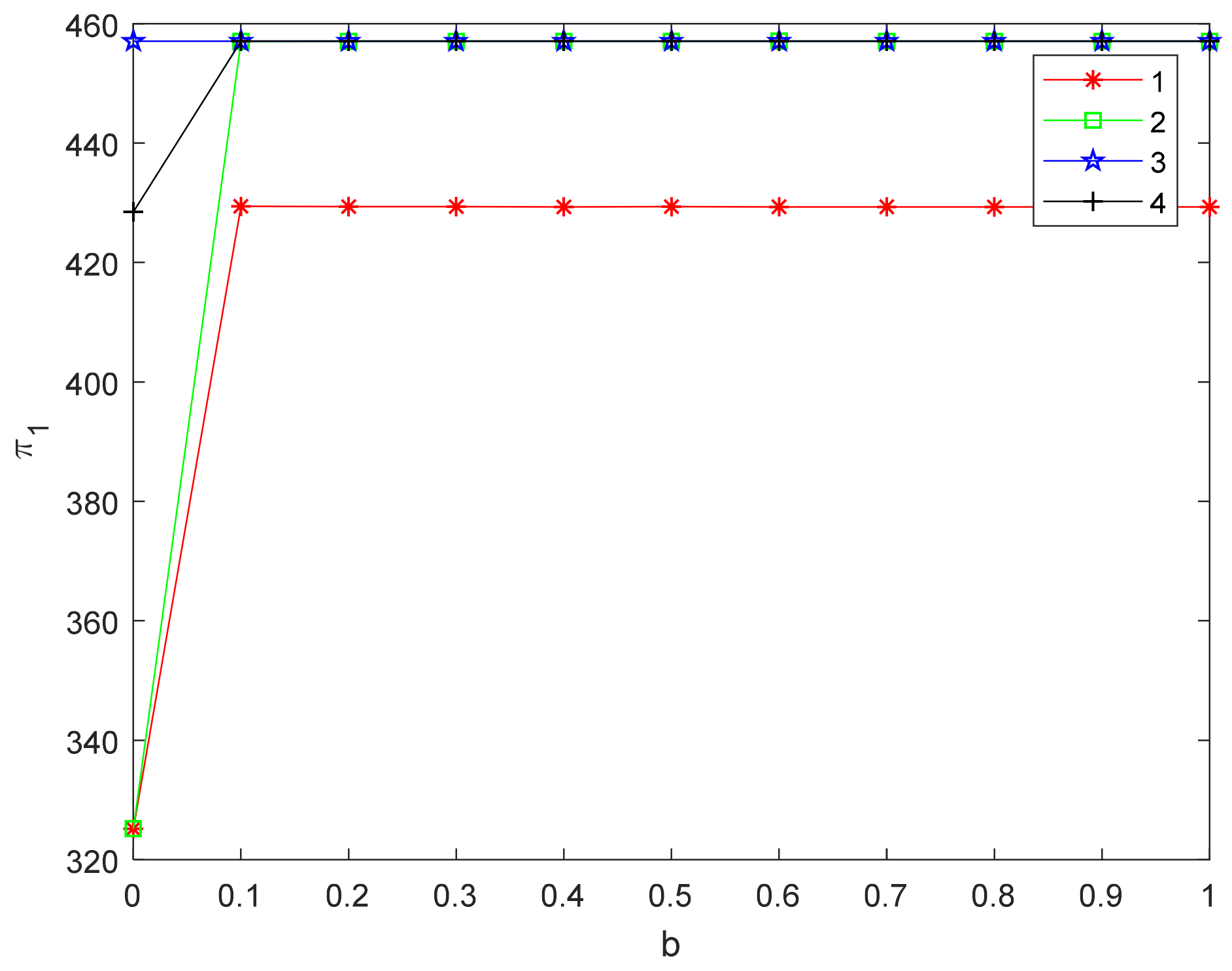
It can be seen from
Table 7 that the three FLSPs pay more attention to their own revenue, and their distribution ratios are greater, when each FLSP pays different attention to its own revenue and all are not worthy of the average revenue. As FLSP1 pays more attention to its own revenue beyond the revenue itself, it has a great ratio in the supply chain’s utility. At this time,
is relatively great and the effort level is relatively great, which can create more value-added. It can be seen from
Figure 14 that
decreases with the increase of the inequity aversion’s degree,
, while the ratios of other FLSPs increase when FLSP1 begins to pay attention to the fairness of revenue distribution. When
is the same as the average, the distribution scheme is no longer affected by
.
changes according to the change of its
, while
changes are the opposite from
Figure 13. If LSI wants to get more revenue, it should cooperate with FLSPs who have inequity aversion.
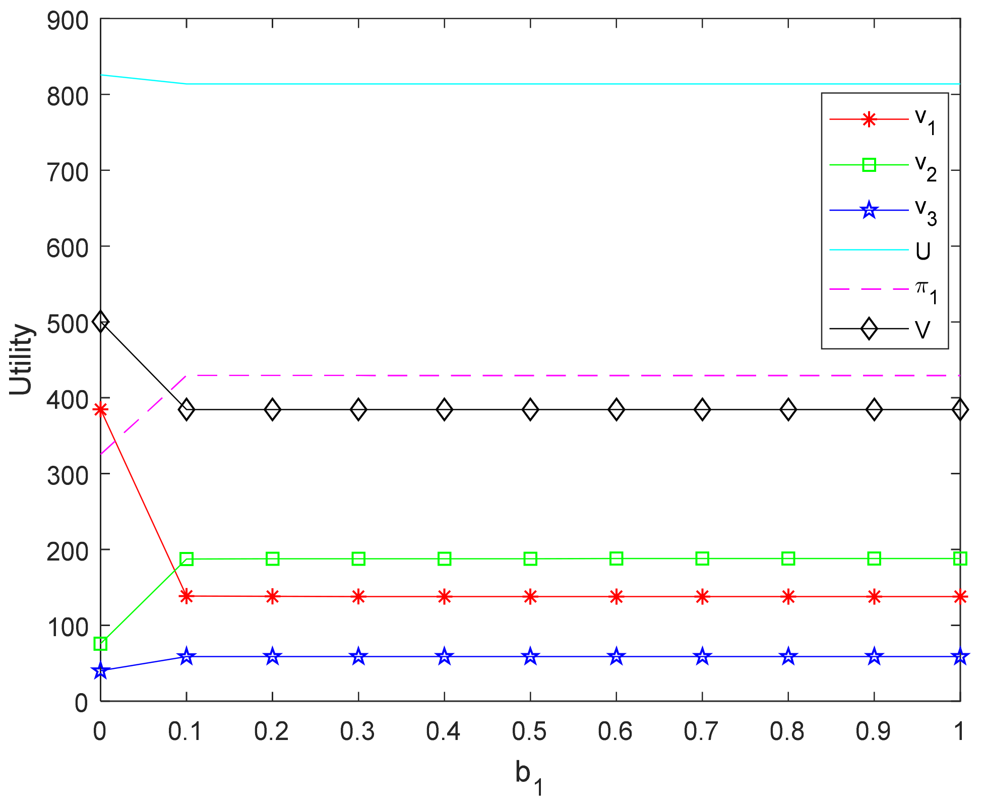
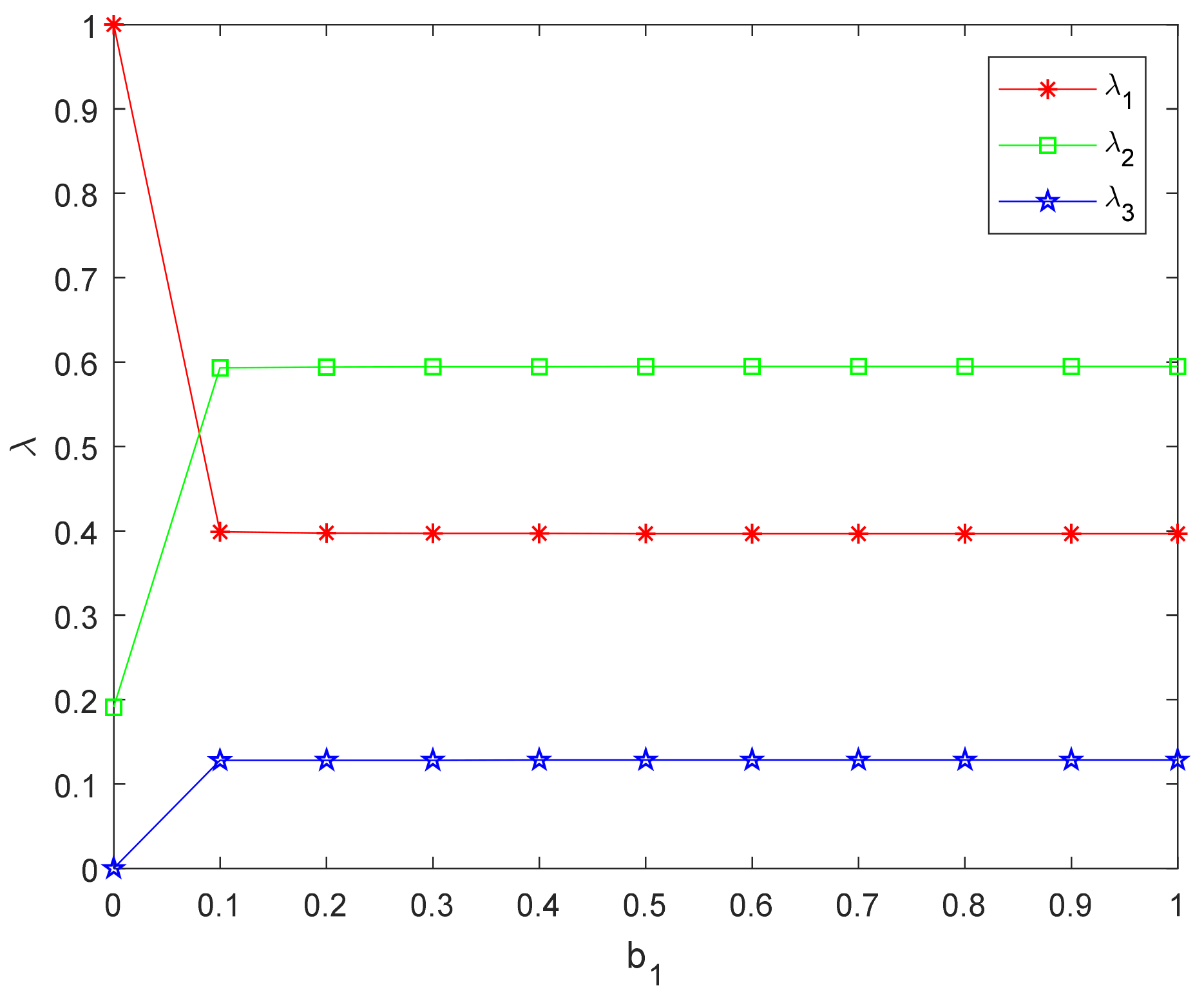
Situation 2.
Fair-neutral FLSPs account for the minority.
For situation 2, the inequity aversion parameters of the three FLSPs are
and
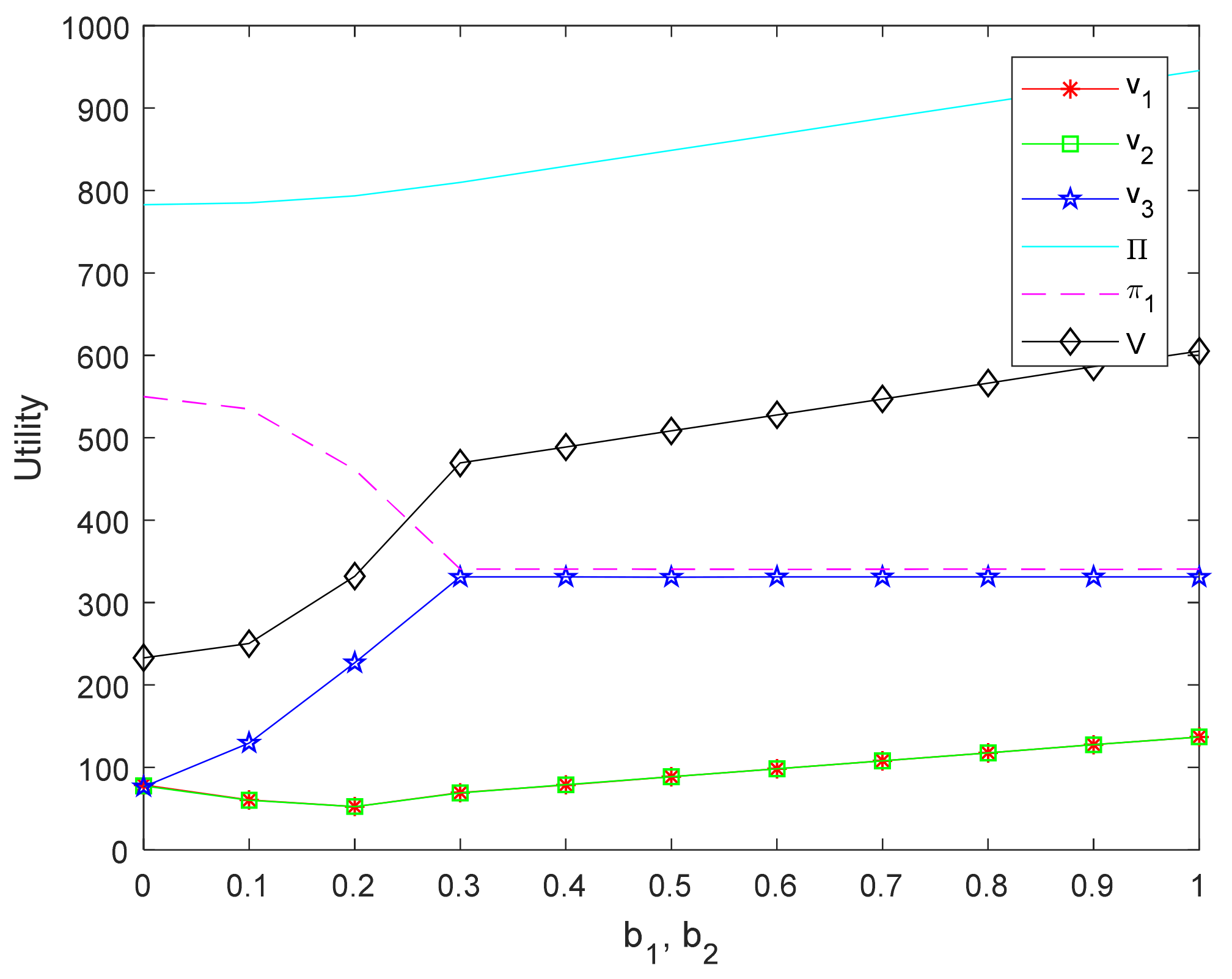
, where only FLSP3 is fair-neutral. The experiments are carried out by changing the value of inequity aversion parameters of FLSP1 and FLSP2,
and
, from 0 to 1, respectively. The results of experiments are shown in
Table 8,
Figure 15 and
Figure 16.
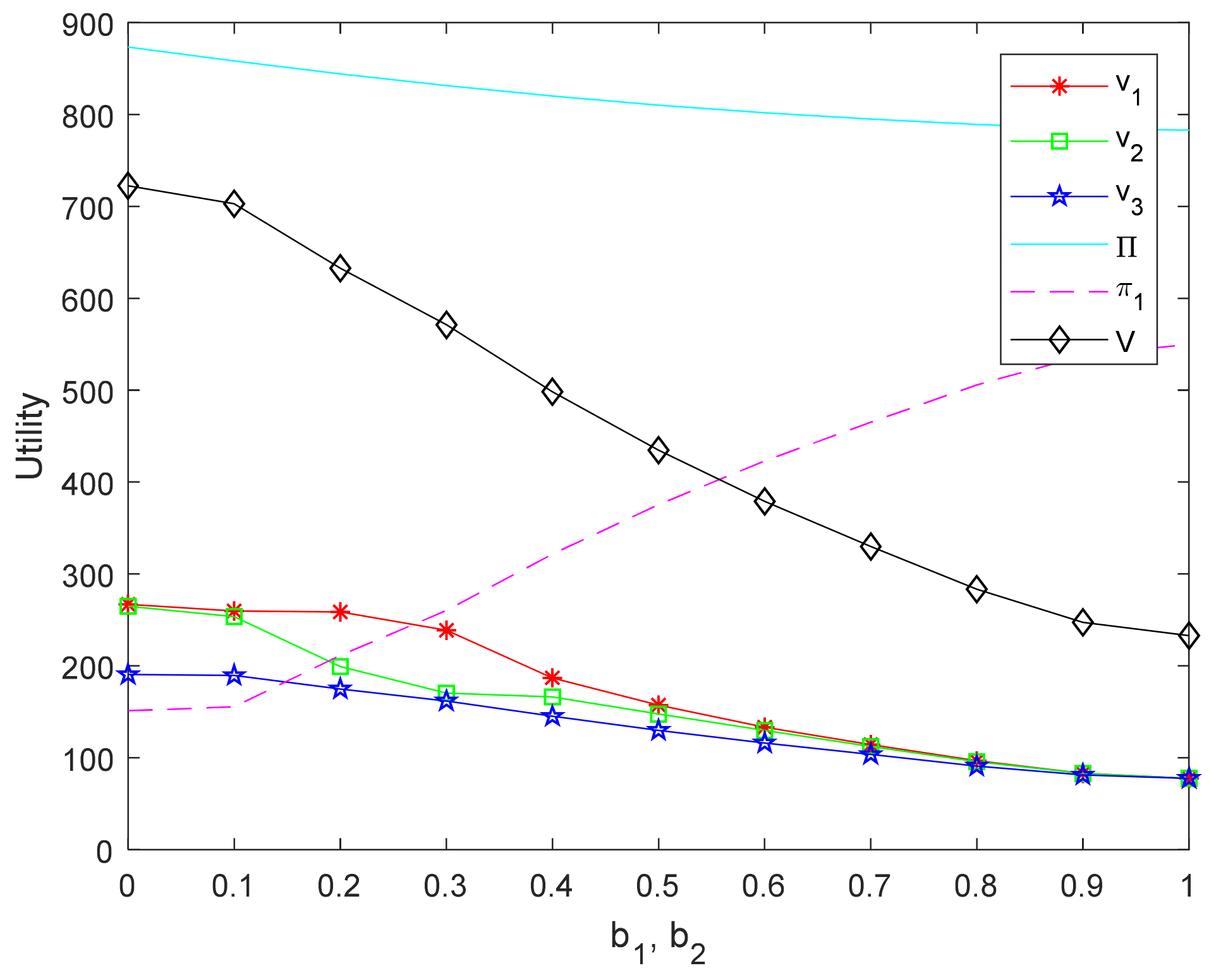
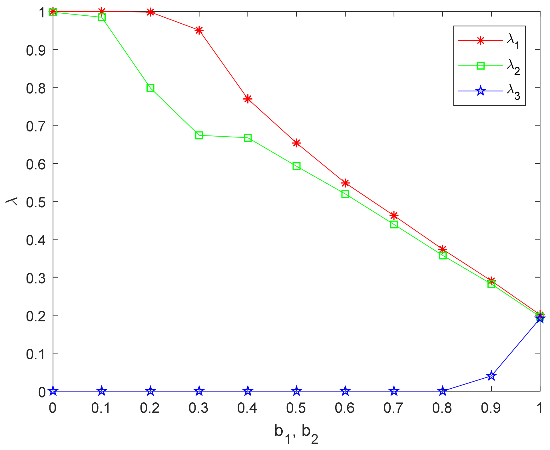
It can be seen from
Table 8 that FLSP2 begins to have disadvantageous inequity aversion,
and
increase with the degree of inequity aversion, when the degree of members’ inequity aversion is weak. From
Figure 15, FLSP2 has advantageous inequity aversion while
increases beyond the average level. As shown in
Figure 16,
decreases and
decreases when the degree of inequity aversion increases. The changes in the remaining members are roughly the same as those in the case 1 and will not be repeated.
Compared with Situation 2 in
Section 4.3.2, the improved BO model is used to increase the distribution ratio and utility of the disadvantaged FLSP when the degree of inequity aversion is strengthened and reduce the distribution ratio and make the revenue distribution fairer for an advantageous FLSP. It can be clearly seen that the improved BO model can better portray the inequity aversion of members and lead to a fairer revenue distribution plan.
- (2)
Extremely inequity aversion FLSPs among members
Situation 3.
Extremely inequity aversion FLSPs account for the majority.
For situation 3, the inequity aversion parameters of the three FLSPs are
,
, where FLSP2 and FLSP3 are extremely inequity aversion. The experiments are carried out by changing the value of inequity aversion parameters of FLSP1,
increases from 0 to 1. The results of experiments are shown in
Table 9 and
Figure 17 and
Figure 18.
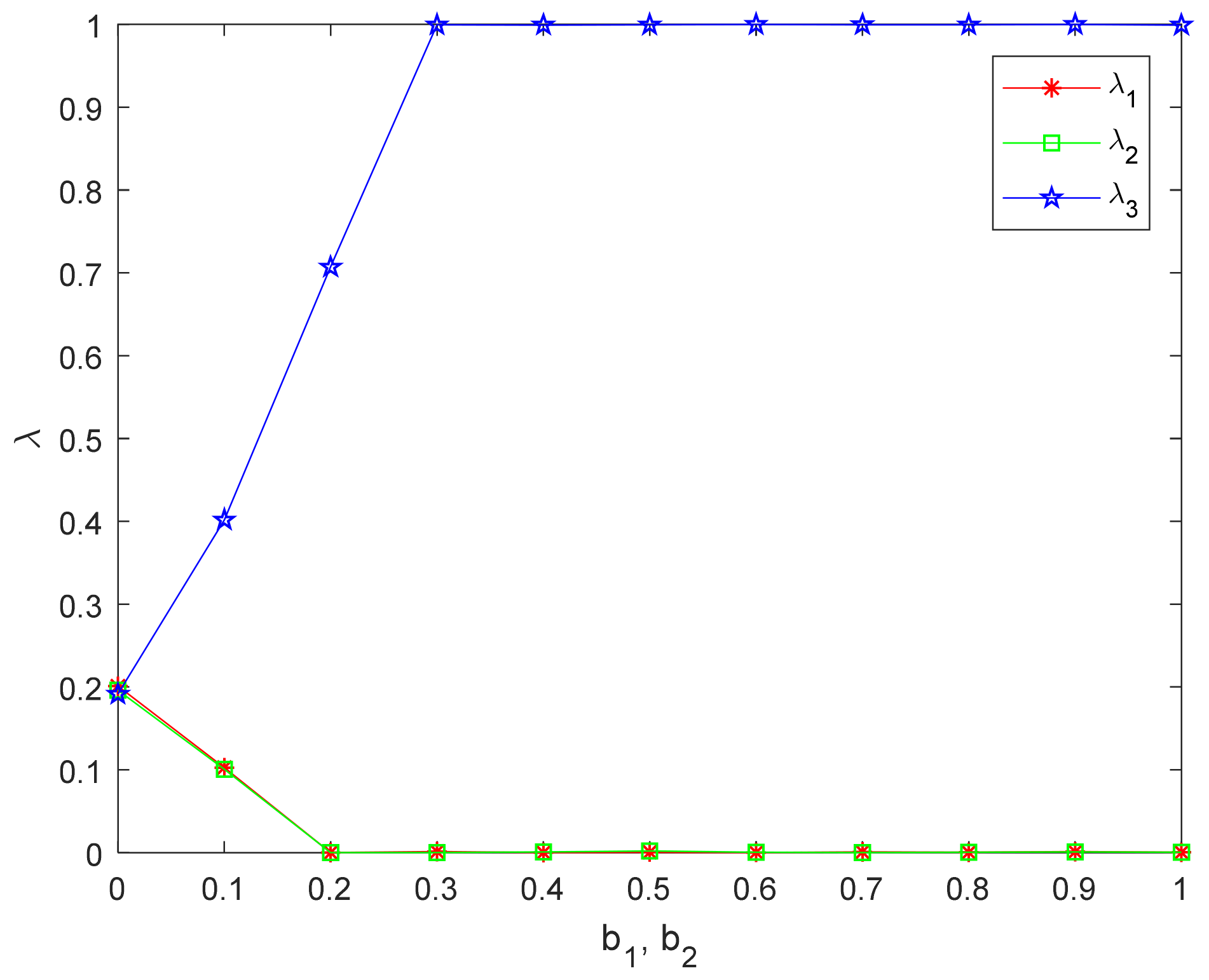
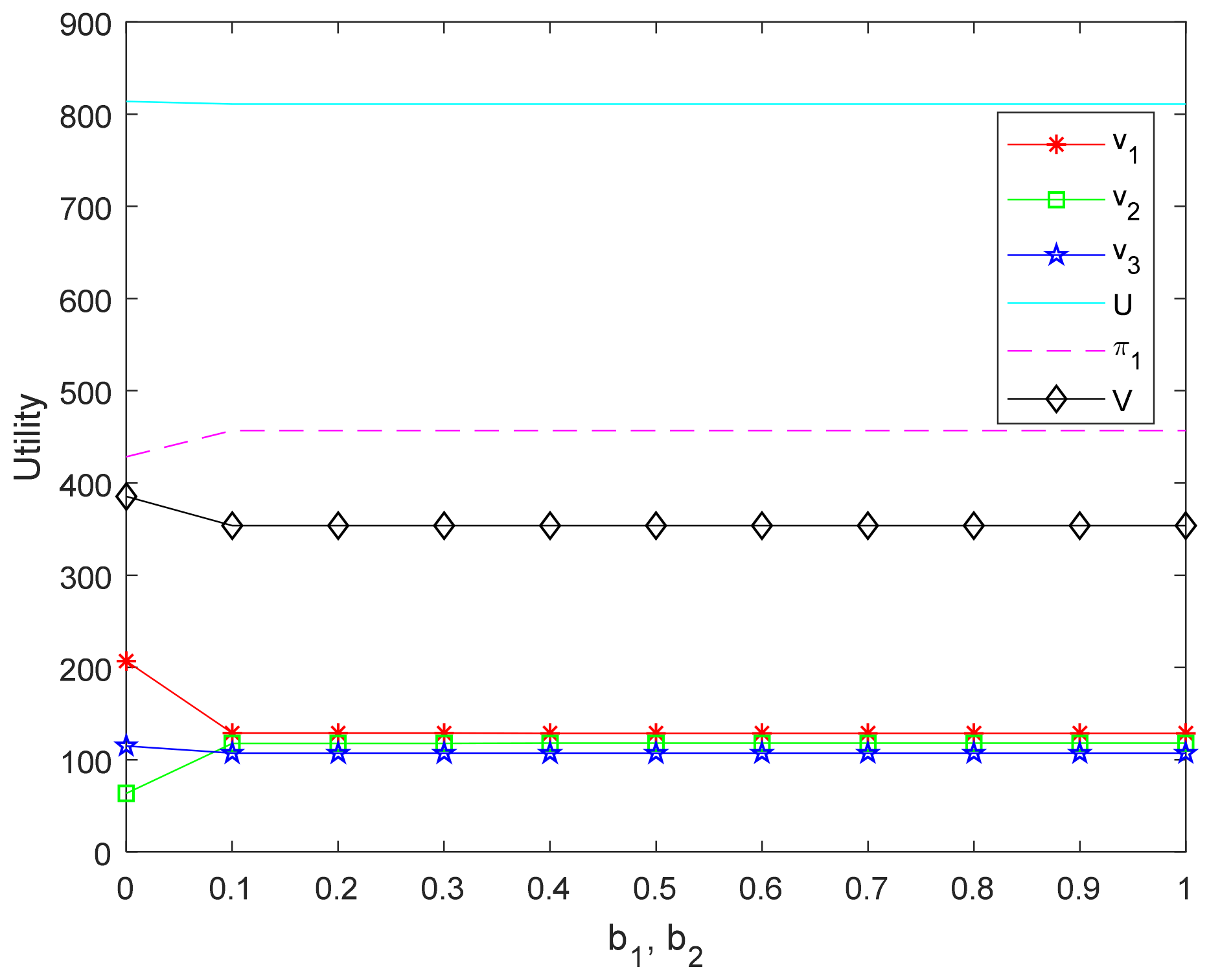
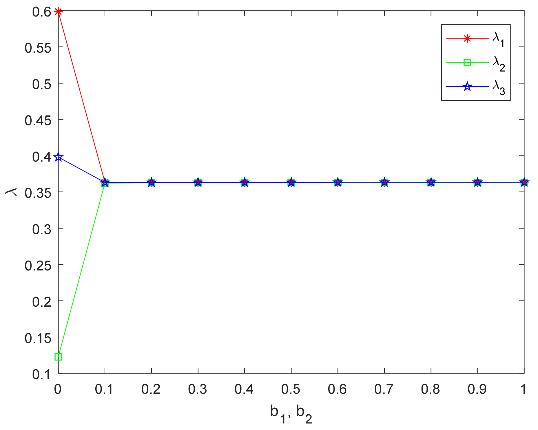
It can be seen from
Table 9 and
Figure 17 the distribution ratios of the three FLSPs are similar, and the utility changes are small when the members with extremely inequity aversion are in majority.
Figure 18 indicates that the FLSP1′s distribution ratio,
decreases and the distribution ratios of other FLSPs increases, which is consistent with the trend of the previous two cases, when the advantageous FLSP1 inequity aversion becomes stronger. This is because more members pay attention to the fairness of distribution. In order to reduce the negative utility caused by inequity aversion, all FLSPs have similar distribution ratios and their profits are roughly the same as shown in
Figure 17 and
Figure 18. In this case, the utility of LSI does not change much.
Compared with situation 3 in
Section 4.3.2, with the original model, the ratio of members with extremely inequity aversion is extremely low, and the ratio of members with weak degrees of inequity aversion is high. With the improved BO model, the ratio of members who are extremely inequity aversion is appropriate, and the profit are the same as the average. For the FLSP with advantageous position, when its degree of inequity aversion is strengthened, its distribution ratio is reduced, and the distribution ratio of members who are extremely inequity aversion is increased, so that the distribution of revenue is fairer.
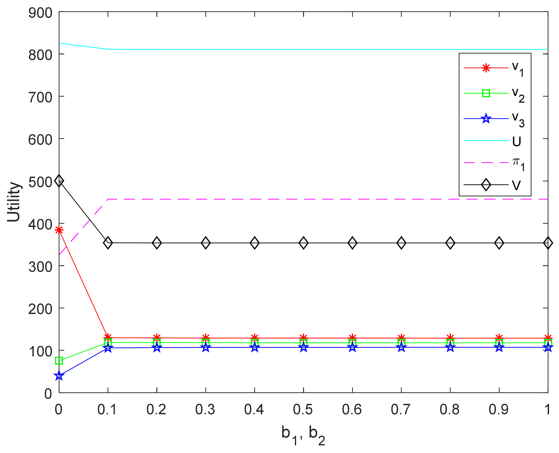
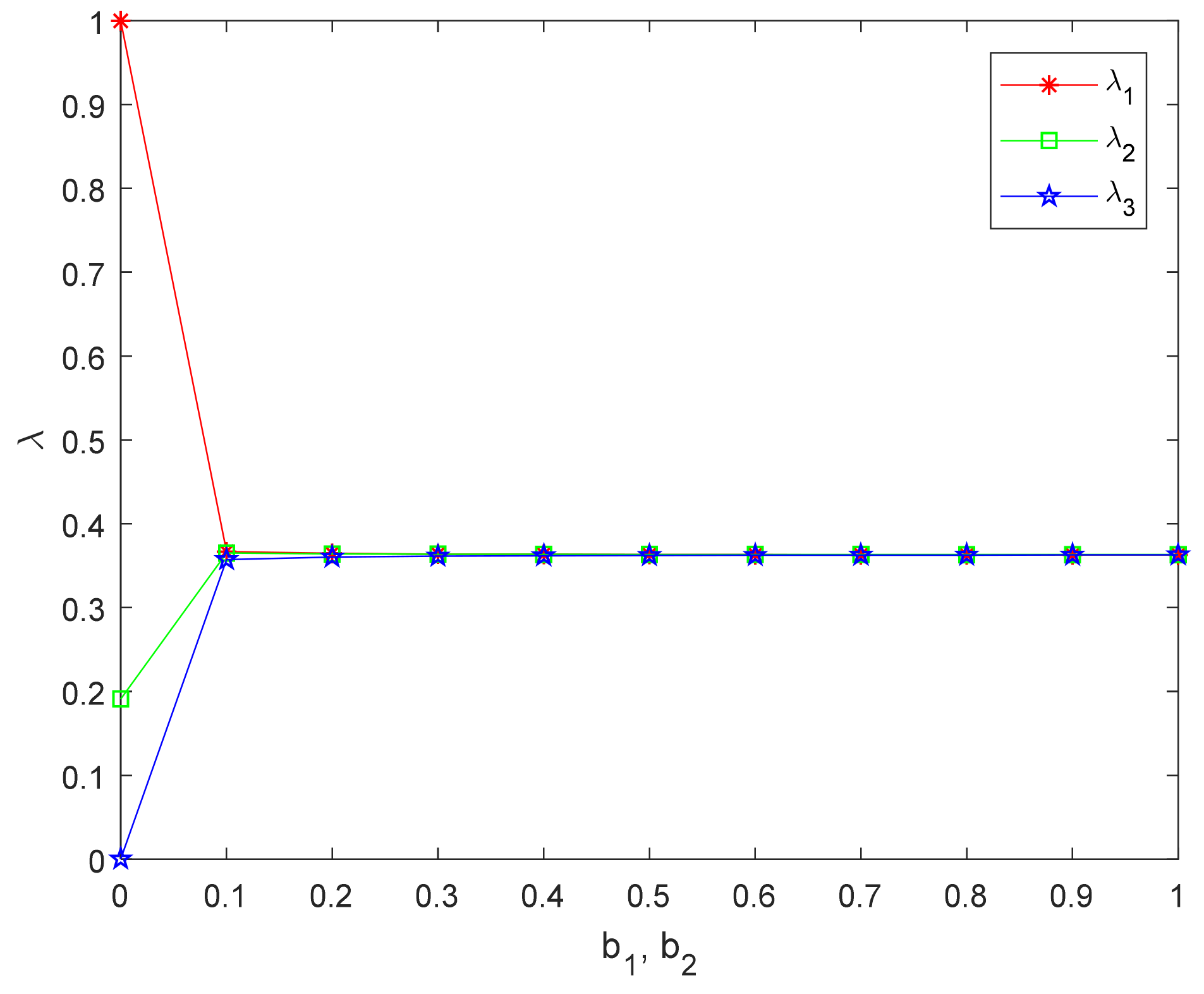
Situation 4.
Extremely inequity aversion FLSPs account for the minority.
For situation 4, the inequity aversion parameters of the three FLSPs are
,
, respectively, where FLSP3 is extremely inequity aversion. The experiments are carried out by changing the value of inequity aversion parameters of FLSP1 and FLSP2,
and
, from 0 to 1, respectively. The results of experiments are shown in
Table 10,
Figure 19 and
Figure 20.
It can be seen from
Table 10 and
Figure 19 and
Figure 20 that situation 4 is roughly the same as situation 1 and situation 2 when member with extreme inequity aversion is the minority. However, FLSP3 is more concerned about the distribution fairness, and FLSP2 is less concerned with its own revenue than FLSP1, and FLSP1 is less inequity averse than FLSP2 at the beginning. As can be seen from situation 1, FLSP1 has an advantage in the whole. Therefore, as described in
Figure 20, FLSP2 has the lowest distribution ratio and FLSP1 has the highest distribution ratio. Similar to situation 2, FLSP2 is below average,
increases with its disadvantageous inequity aversion,
, in
Figure 20, and
is higher than the average in
Figure 19.
decreases with its advantageous inequity aversion.
Figure 20 demonstrates that the distribution ratio is no longer affected by the degree of inequity aversion, while the members’ revenues are almost the same.
Compared with Situation 4 in
Section 4.3.2, with the original model, the ratio of members who are extremely inequity aversion is extremely low. With the improved BO model, the ratio of members who are extremely inequity aversion is appropriate, and the profit is the same as the average. For the disadvantageous FLSP, when its degree of inequity aversion is strengthened, the ratio of its distribution is appropriately increased to increase its utility. For the advantageous FLSP, reduce the distribution ratio and make the revenue distribution fairer.
- (3)
Experimental summary
Comparing the utility of supply chain and the profit of LSI in the four situations,
Figure 21 shows that the supply chain has the greatest utility when all members are fair-neutral. As can be seen from
Figure 21 and
Figure 22, the smaller
are, but the greater
are, when the more members pay attention to the fairness of distribution and the stronger the degree of inequity aversion is. This is because when FLSP focuses on the distribution of fairness, it will have a negative effect whether it is below or above the average. This indicates that the distribution ratios agreed between LSI and the three FLSPs should be similar to seek a fairer trade, and LSI has to work harder to get more revenue.
Compared with the four situations in
Section 4.3 above, the experimental results in this section are obviously different. Applying the improved BO model, there is no unreasonable situation in which the ratio of revenue distribution is lower and the utility is increased, when the FLSP has disadvantageous inequity aversion. The improved BO model can successfully describe the advantageous inequity aversion and disadvantageous inequity aversion of FLSP. Applying the improved BO model, the revenue distribution plan is fairer, more reasonable and more realistic. The improved BO model is suitable for situations where the specific information of peer members is not fully known, but the industry average is known, and
can be adjusted according to the capabilities of the company.
5.2.2. Influence of Relative Fairness Revenue Coefficient on Revenue Distribution
In order to study the influence of the relative fairness revenue coefficient of FLSPs on the distribution scheme, the following experiment was conducted. There are two cases, (1) the members’ relative fairness revenue coefficients are the same and (2) the members’ relative fairness revenue coefficients are different. The initial data of the case is the same as in
Section 4.3.1. To avoid the influence of the inequity aversion degree of members affecting the parameter analysis, the inequity aversion of the three FLSPs are the same, and the parameters are set,
and
.
- (1)
Case 1: Members with the same relative fairness revenue coefficients
The relative fairness revenue coefficients of the three FLSPs are the same, since the strengths of the three FLSPs are similar,
is from 0.9 to 1.1 according to papers by Yang et al. (2013) [
51], Katok et al. (2014) [
31] and Wang et al. (2016) [
48]. The results are shown in
Table 11 and
Figure 23 and
Figure 24.
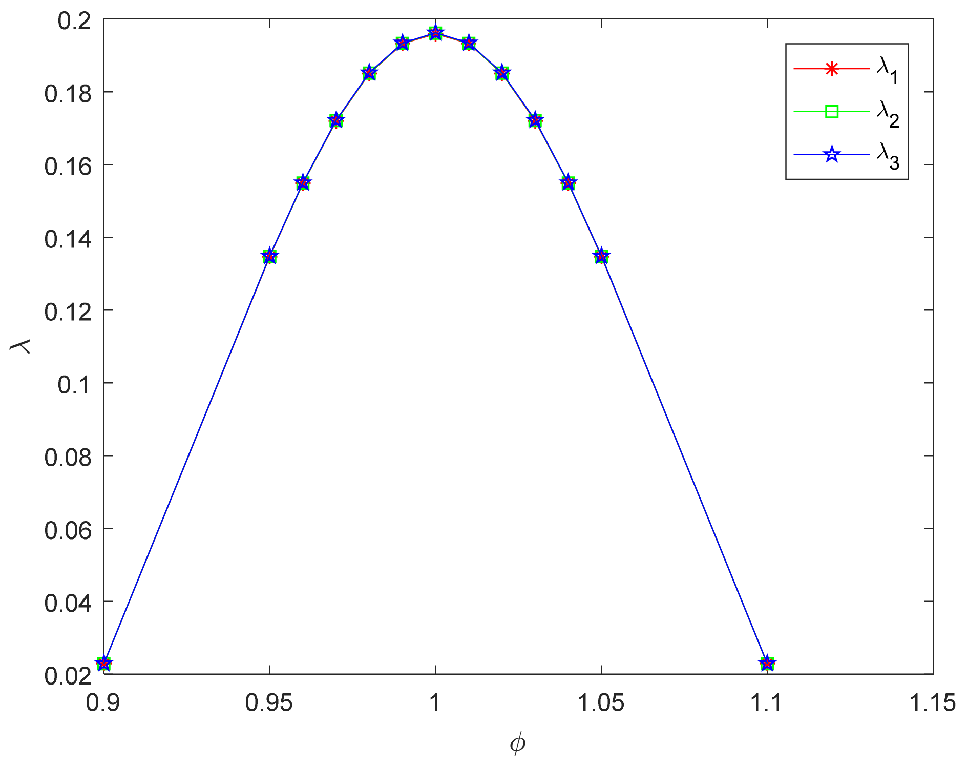
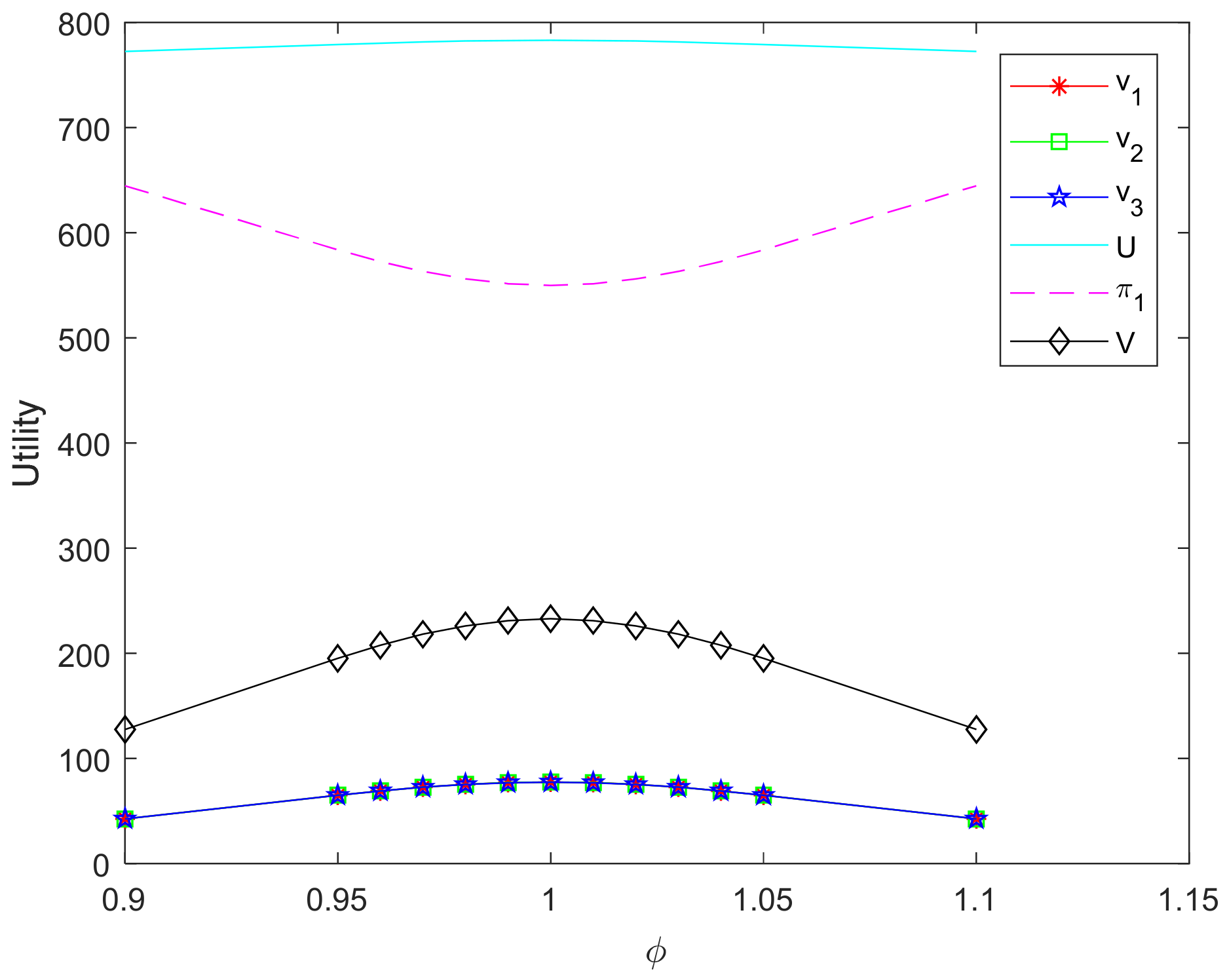
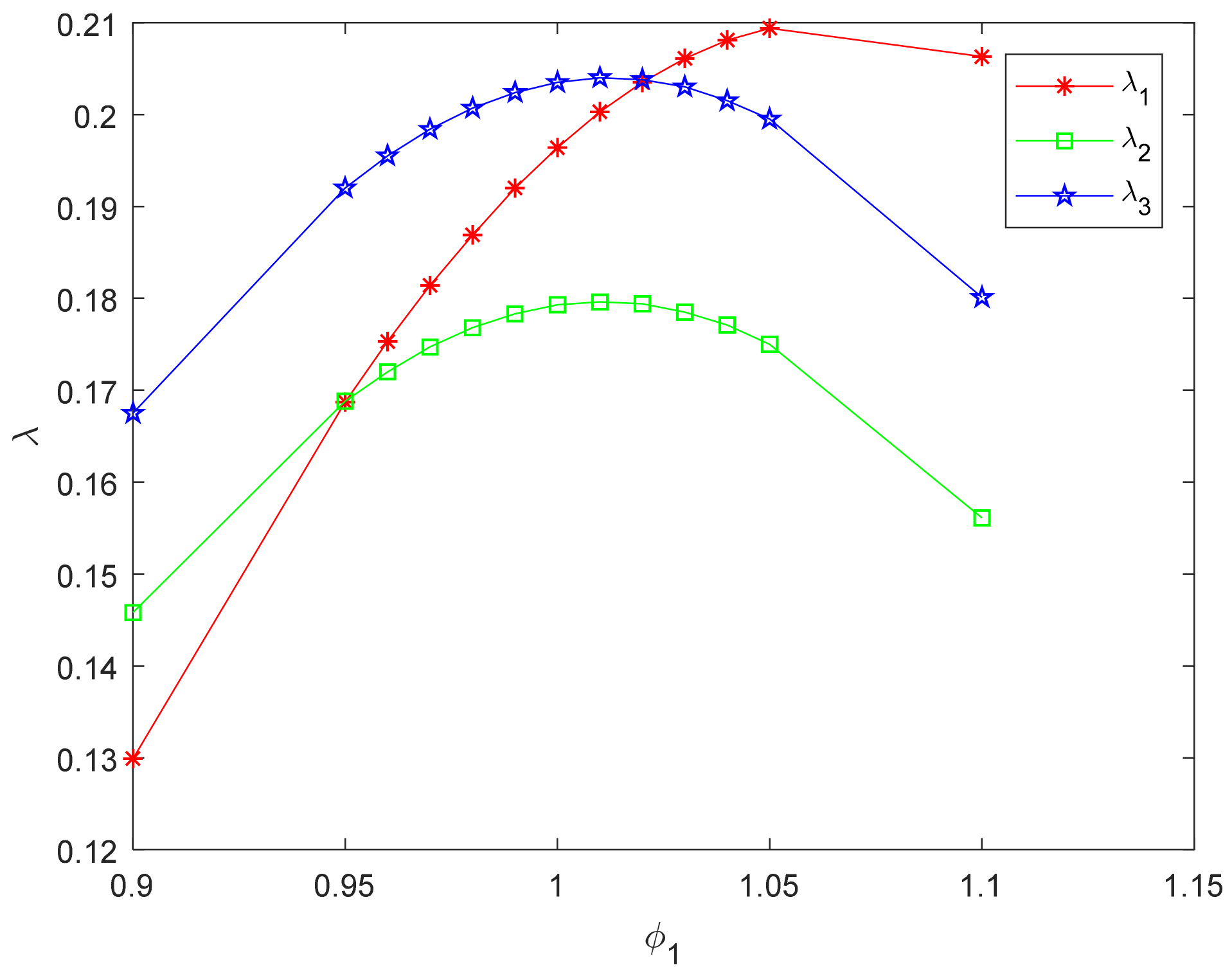
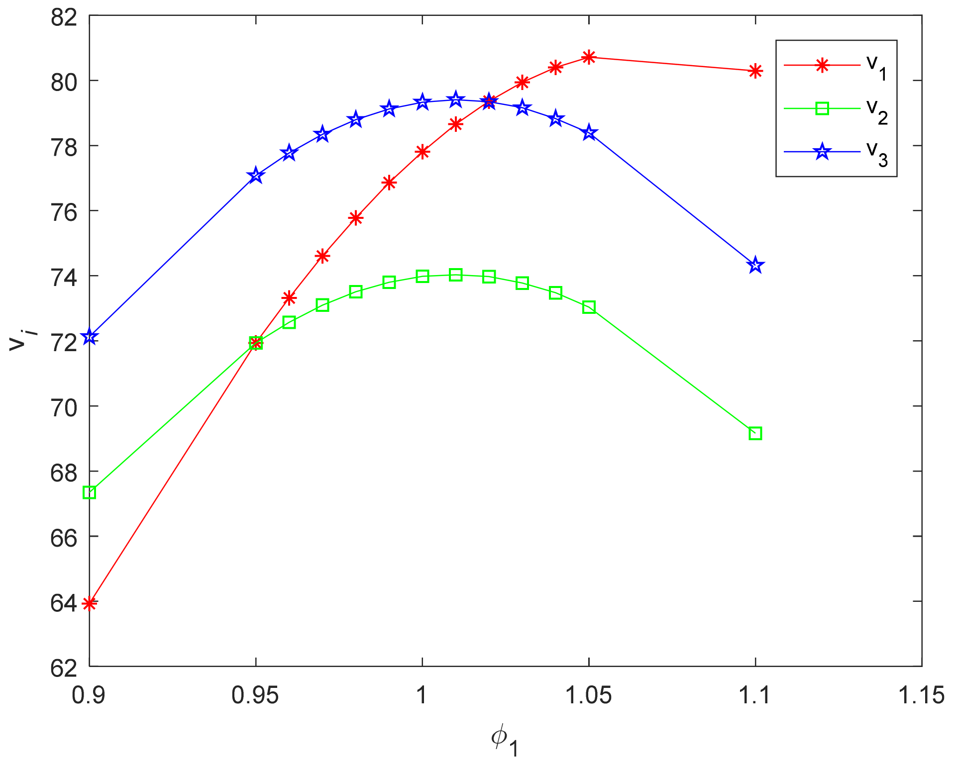
It can be seen from
Table 11 and
Figure 23 that the relative revenue coefficient
makes the FLSP member distribution ratio the highest when the relative fairness revenue coefficients of the three FLSPs are the same. At this time,
,
and
are the highest in
Figure 24.
Figure 24 also indicates that
and
will decrease when the relative fairness revenue coefficient
increases or decreases.
- (2)
Case 2: Members with different relative fairness revenue coefficients
The relative fairness revenue coefficients of the three FLSPs are different,
from 0.9 to 1.1,
, which means that the strength of the FLSP 2 is lower than the average, and
, which means that the strength of the FLSP 3 is higher than the average [
31]. The selection of member whose
is changed is random, and the values of
and
are set only to express the difference in FLSPs’ strength, which will not affect the final conclusion [
52,
53,
54]. The results are shown in
Table 12 and
Figure 25 and
Figure 26.
As can be seen from
Table 12 and
Figure 25, the distribution ratio of FLSP1 is lower than that of other FLSPs,
, when
. With increases of
,
increases gradually, which is shown in
Figure 25. FLSP1 and FLSP2 have the same revenue distribution ratio, which is smaller than the distribution ratio of FLSP3,
when
. The distribution ratio of FLSP1 is higher than other FLSPs,
when
. It can be concluded that the higher the relative fairness revenue coefficient of the FLSP is, the higher the distribution ratio is in the peer FLSPs.
Figure 26 shows that the trend of the utility of FLSP is the same as the distribution ratio.
Comparing
Figure 23 with
Figure 25, it can be seen that
that can make the ratio of member greatest have a deviation when the members have different relative fairness revenue coefficients. This is because the benchmark for comparison with the average level increases when a member’s relative fairness revenue coefficient increases. LSI increases the distribution ratio and compensates for the inequity negative utility resulting from comparison.
- (3)
Experimental summary
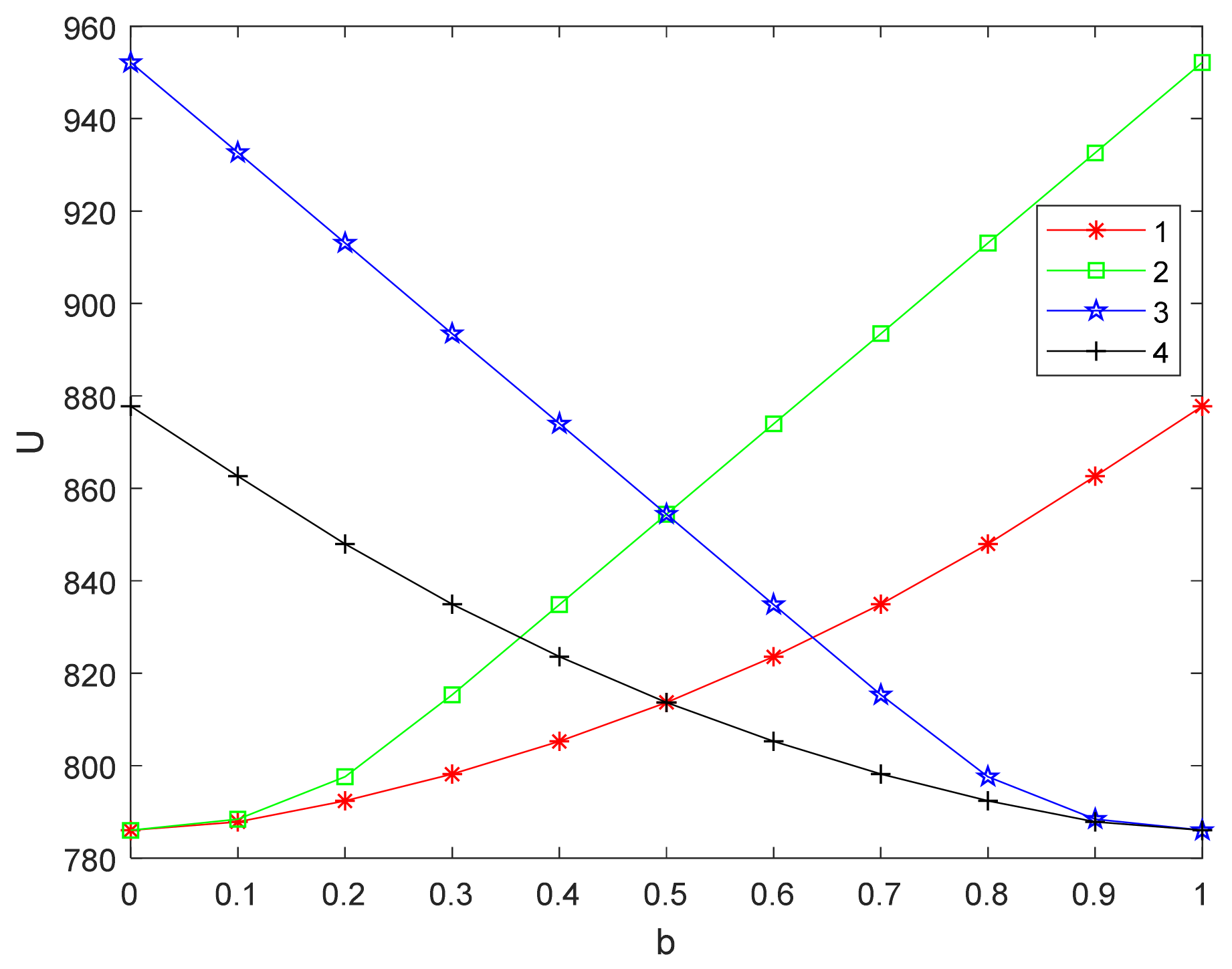
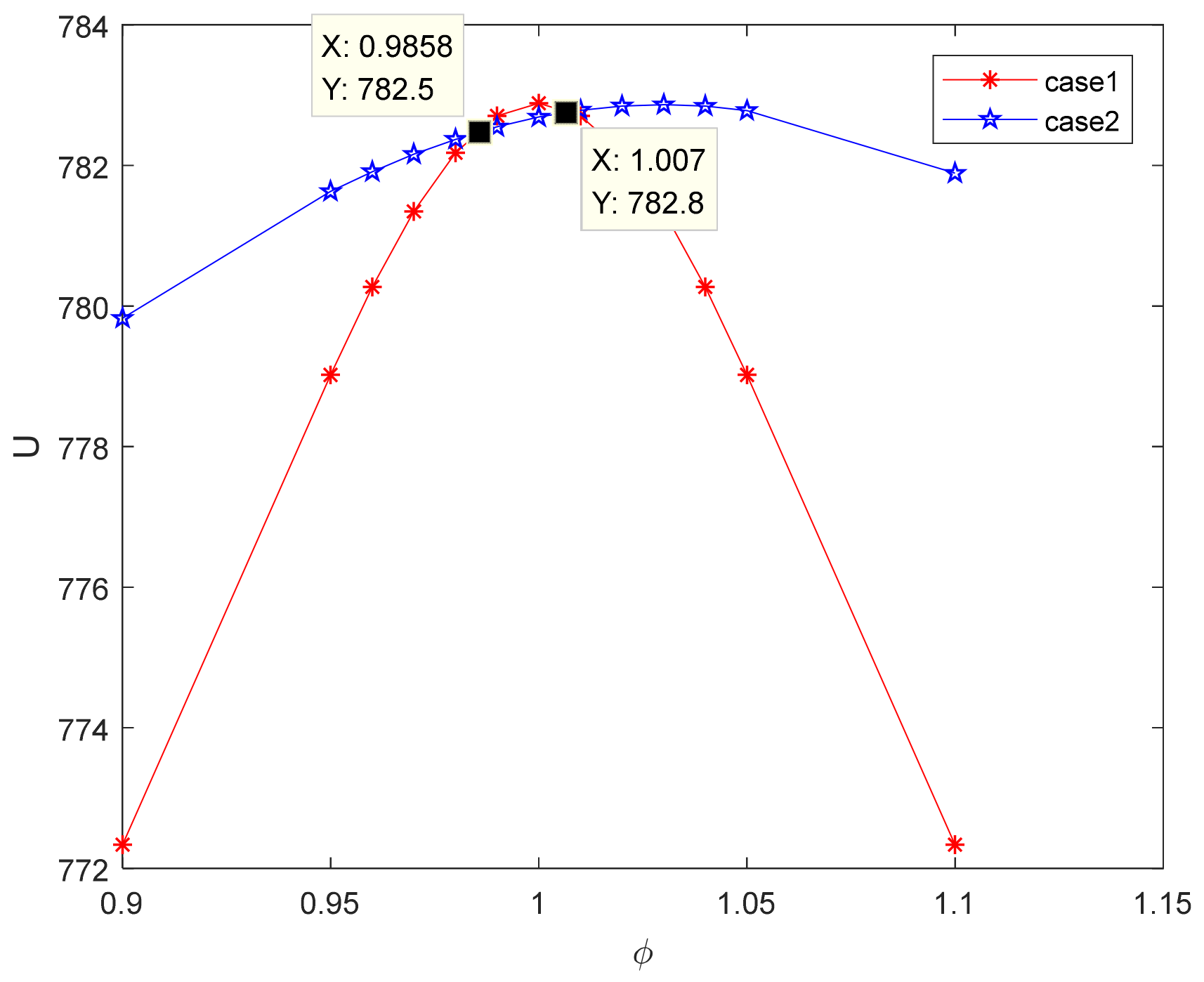
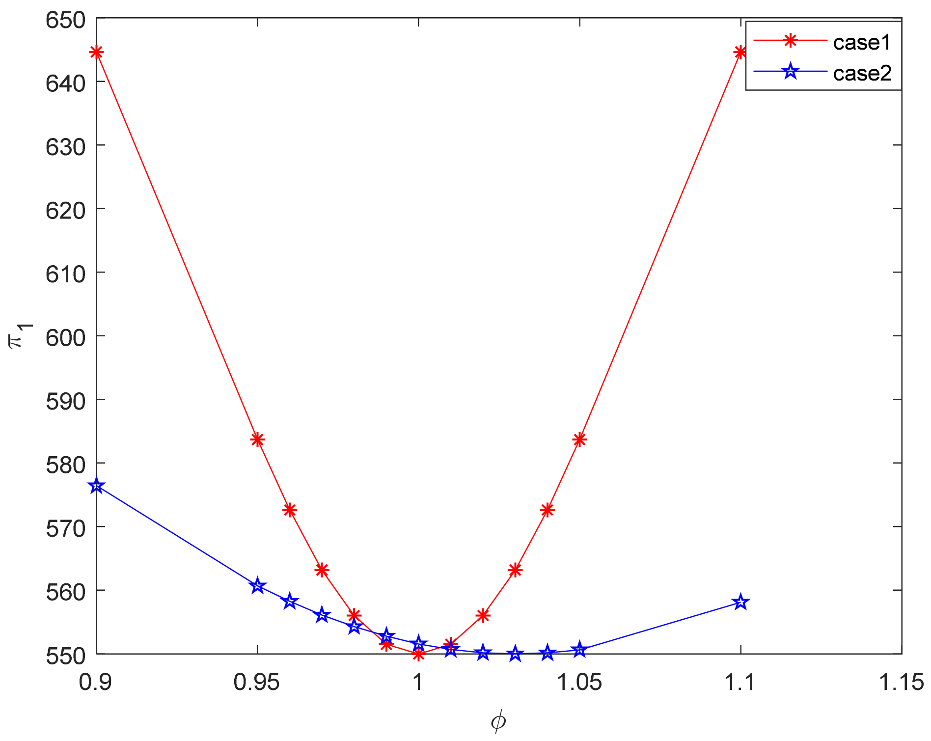
Comparing the utility of the two types of experiments, it can be seen from
Figure 27 and
Figure 28 and
of case 1 are equal to that of case 2 when
and
; when
,
and
of case 1 are greater than that of case 2, where the differences between the
of the FLSPs in Case 2 is small; when
and
,
and
of case 1 are smaller than that of case 2, where the differences between the
of the FLSPs in Case 2 is great.
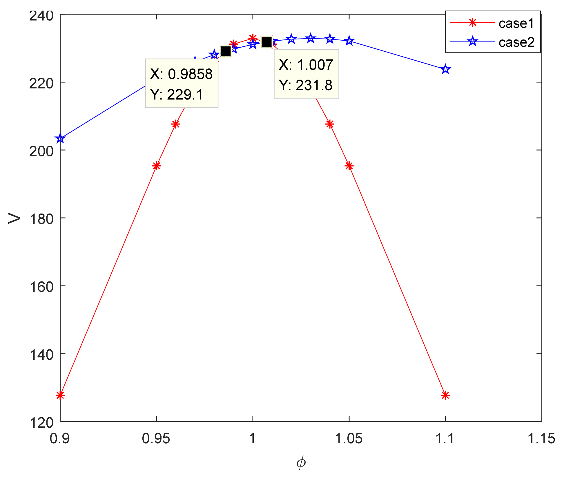
Figure 29 shows that the comparison result of
in both cases is contrary to the comparisons of
and
.
denotes the degree of FLSP
i’s perceived relative advantage against the peers and the status of FLSP in the peers, and depends on the factors such as the fixed cost, efficiency and innovation capability of the enterprise, etc. Specifically, the larger the FLSP
i’s perceived relative advantage against the peers is, the stronger the strength of FLSP among their peers is, the bigger the
will be. The greater the difference in the
between FLSPs is, the greater the gap in the strength of FLSP is. If LSI only pursues to maximize its own interests, she can choose to cooperate with FLSPs with the same strength and whose strength is greater or lesser than average. When LSI cooperates with FLSPs with large differences in strength, she should give more powerful FLSPs higher distribution ratios to encourage them to create more value and reduce the ratios of weaker FLSPs.


