Assessment of Emission Reduction and Meteorological Change in PM_2.5 and Transport Flux in Typical Cities Cluster during 2013–2017

Abstract

Under the Air Pollution Prevention and Control Action Plan (APPCAP) implemented, China has witnessed an air quality change during the past five years, yet the main influence factors remain relatively unexplored. Taking the Beijing-Tianjin-Hebei (BTH) and Yangtze River Delta (YRD) regions as typical cluster cities, the Weather Research Forecasting (WRF) and Comprehensive Air Quality Model with Extension (CAMx) were introduced to demonstrate the meteorological and emission contribution and PM_2.5 flux distribution. The results showed that the PM_2.5 concentration in BTH and YRD significantly declined with a descend ratio of −39.6% and −28.1%, respectively. For the meteorological contribution, those regions had a similar tendency with unfavorable conditions in 2013–2015 (contribution concentration 1.6–3.8 μg/m³ and 1.1–3.6 μg/m³) and favorable in 2016 (contribution concentration −1.5 μg/m³ and −0.2 μg/m³). Further, the absolute value of the net flux’s intensity was positively correlated with the degree of the favorable/unfavorable weather conditions. When it came to emission intensity, the total net inflow flux increased, and the outflow flux decreased significantly across the border with the emission increasing. In short: the aforementioned results confirmed the effectiveness of the regional joint emission control and provided scientific support for the proposed effective joint control measures.

1. Introduction

During the past years, a severe widespread air pollution event with high concentrations of PM_2.5 occurred in most cities’ development process such as Beijing-Tianjin-Hebei (BTH) and Yangtze River Delta (YRD) that gradually became the main economic entities attracting worldwide attention [1,2]. Severe PM_2.5 pollution became a critical concern and urgent challenge for the government and public [3,4,5,6]. It not only posed a threat to human health and sustainable development but also influenced the atmospheric visibility and climate systems [7]. Take 2013 for example, the annual average PM_2.5 concentrations in the BTH and YRD regions reached 105 and 68 μg/m³, which were nearly 2–3 times higher than China’s National Ambient Air Quality Standard (NAAQS) of 35 μg/m³ [8,9]. In fact, the Chinese government established the Air Pollution Prevention and Control Action Plan (APPCAP) in September 2013 in order to mitigate the increasingly severe PM pollution in China, especially in typical regions. Based on the guidance of the APPCAP, each typical city made further efforts to mitigate air pollution. After implementing a set of air pollution control policies, the average PM_2.5 concentrations in BTH and YRD dropped to 65 and 48 μg/m³ by 2017, respectively [10,11]. Meanwhile, adjacent areas, such as the Shandong, Shanxi, and Henan provinces, also released the APPCAP, with the whole region attaining remarkable improvements in air quality, which were also verified by satellite-based and ground-based observations [12,13,14,15].

As is well known, local pollutant emission was the main contribution source for a given city, and control responding to the local pollutant has always been one of the most effective methods to improve the air quality [16]. Meanwhile, the regional transport should not be overlooked, BTH is embraced on three sides by mountains which easily transport air pollutants from the south and southeast direction with Shijiazhuang and Tangshan being heavy industry cities, while YRD is the largest foreign trade export port and possesses a full range of industrial parks, which are affected significantly by the sea breeze and land breeze transport of air pollutants [17,18]. The regionally complex air pollution characteristics resulted from the PM_2.5 formation and transport [19,20]. By emission inventories and air quality models, several studies established a mature sensitivity decomposition framework to assess the contribution of emission control to air quality improvements but neglected the influence above the regional transport, especially in different heights [21]. Therefore, it was essential to acquire a deep understanding of the characteristics of the fine particulate matter and their species and quantitatively evaluate the transport characteristics of the pollutants.

The decreasing concentration of PM_2.5 pollution in the BTH and YRD regions was significant during 2013–2017. Those phenomena resulted from the integrated effects of various factors, such as the local emission control, the surrounding emission reductions, and meteorological condition changes. Previous studies studied the roles of the meteorological conditions as well as local emissions; however, the aforementioned researchers analyzed one single factor or took heavy pollution episodes into consideration. Thus, large gaps remained in the knowledge pertaining to the BTH and YRD regions’ air quality improvements through the systematic and decomposed attribution analysis, especially during the periods of 2013–2017, when the PM_2.5 in the above mentioned decreased significantly, let alone the influence of the regional transport [22,23,24].

To address this knowledge gap, a more comprehensive analysis of the period of 2013–2017 is urgently necessary. In this paper, we investigated the impacts of local policies and the meteorological changes on PM_2.5 abatements in the BTH and YRD regions during 2013–2017, based on several sensitivity simulations and regional transport flux changes due to former factors, via the transport flux model. First, the emission reductions of the BTH and YRD regions were assessed based on the quantification of air pollution control measures. Second, based on the single variable principle, we designed a serious sensitivity scenario simulation under different local emission controls and different meteorological conditions. Third, we applied the Weather Research and Forecasting Model and Comprehensive Air Quality Model to reproduce air pollutant temporal and spatial distribution. Finally, based on the model and transport flux method, an integrated and decomposed attribution analysis of the PM_2.5 concentration and its transport flux in the BTH and YRD regions was developed to quantify the influence from the local pollution control and meteorological changes.

2. Materials and Methods

First, we applied the observation data from the China National Environmental Monitoring Center (CNEMC, http://106.37.208.233:20035/, accessed on 28 February 2021) of the national observation station in the main provincial capital to review the air quality during 2013–2017, especially the monthly PM_2.5 concentrations in this period. The two main factors of meteorology change and emission control consisted of the contributions of the total PM_2.5 abatements in those two cities clusters in the period. Then the WRF-CAMx modeling system was applied, and observed PM_2.5 concentrations to quantify the contributions of the two factors.

2.1. Measurement Data

Firstly, we reviewed the air quality in those two cluster cities from 2013 to 2017 with ground observation data (496 sites in 74 major cities in 2013 and ~1500 sites in 454 cities by 2017) [25]. In this study, we reviewed the monthly changes in SO₂, NO₂, CO, O₃, PM_2.5, and PM₁₀ during 2013–2017 for the studied areas and analyzed the PM_2.5 concentrations during the same period. Additionally, we evaluated the accuracy of the PM_2.5 composition simulation we conducted, based on URG samplers in Beijing (BJ), Tangshan (TS), and Shijiazhuang (SJZ), located on the building roof roughly 20 m off the ground. Those three samples were part of a long-term project that observed the represent month characters in typical cities since 2013. The samples were collected particular matter mass on the Whatman 41 filters and quartz filters (Whatman, Inc., Maidstone, UK) to analyze water-soluble ions, carbonaceous components and metal elements. Detailed measurements and site information can be found in Wang’s research [26]. In this study, we used the reconstructed daily PM_2.5 speciation data to verify the variation in PM_2.5 compositions in BTH during 2013–2017. Additionally, we collected the observational PM_2.5 compositions from the reported research to check the simulated variations in PM_2.5 compositions in the CAMx model. In Guan et al. [27] research, the PM_2.5 samples were observed and analyzed at YRD, and the chemical composition changes in 2017 were compared. As for meteorological observations, they were obtained from the National Meteorological Information Center (NMIC, http://data.cma.cn, accessed on 28 February 2021), such as the daily average temperature at the height of 2 m (T2), relative humidity at a height of 2 m (RH), and wind speed at a height of 10 m (WS10).

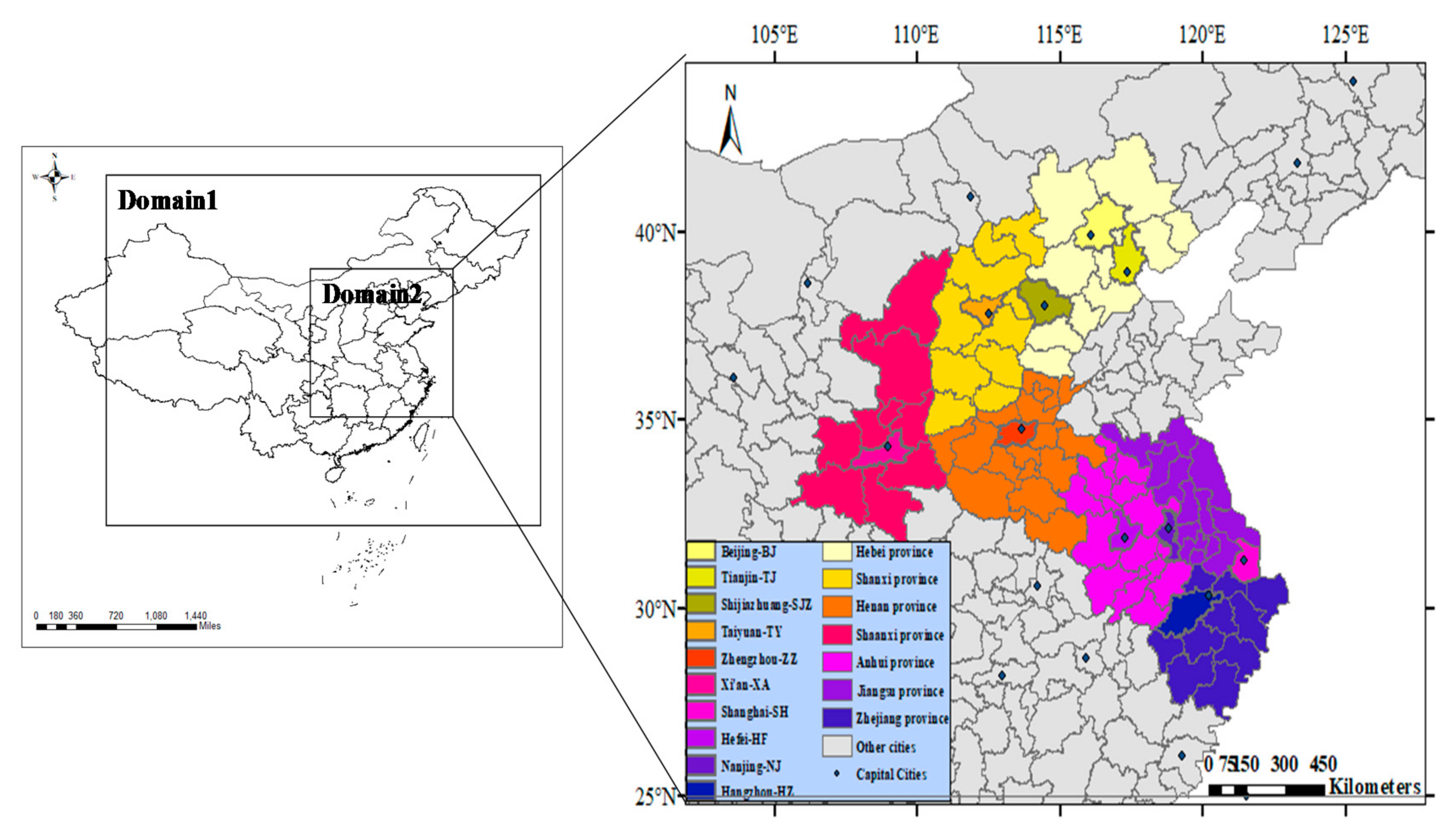
2.2. Model Configuration

In this research, WRFv3.5.1 and CAMx6.3.0 were applied to build up the air-quality modelling system. The WRF model provided the meteorological conditions, while the CAMx model simulated the air quality and main pollutant concentrations. Moreover, for the simulation area, two nested domains were designed in this study (Figure 1), with a horizontal resolution of 36 km × 36 km (120 rows and 171 columns), and 12 km × 12 km (223 rows and 163 columns), respectively. The first domain covered the entire eastern and central area in China, and the second one covered the majority of two cities clusters in China. To reduce the uncertainty of meteorological boundary conditions, the size of the simulation of the CAMx model was three grid cells smaller than that of the WRF model in each domain, with a 10 d spin-up before each period. For the vertical resolution, both WRF simulation and the Meteorology-Chemistry Interface Processor (MCIP) were designed as the same 28 sigma levels from the surface to tropopause (about 100 mbar). The 28 sigma levels for the CAMx model vertical resolution were 1.000, 0.994, 0.988, 0.981, 0.969, 0.956, 0.944, 0.926, 0.902, 0.881, 0.852, 0.828, 0.796, 0.754, 0.704, 0.648, 0.589, 0.546, 0.495, 0.445, 0.387, 0.287, 0.187, 0.136, 0.091, 0.061, 0.020, 0.000. The physical and chemical parameterization schemes of the WRF model have been introduced in detail in our previous studies [27,28]. What is more, the meteorological initial and boundary conditions with a spatial resolution of 1° × 1° and temporal resolution of 6 h were derived from the final analysis data (FNL). For the CAMx model, carbon bond 05 (CB05) was treated as the gas-phase chemical mechanism and AERO6 was applied as the particulate matter chemical mechanism. The chemical initial and boundary conditions were interpolated from the simulated output of the WRF model. January, April, July and October were set as represent month to simulate a time series of all pollutants concentrations during 2013 and 2017 (as base cases), and the modelled 9 sensitivity experiments (described in Section 2.5). Similar configurations for the WRF and CAMx model were introduced in our previous studies and they keep a better agreement with the observations.

2.3. Emissions

The anthropogenic emission data consisted of three parts. The BTH region emission inventory employed a high-resolution county-level pollution emission inventory developed by Zhou et al. [29], the YRD region emission inventory developed by Sun et al. [30], and the emission inventory outside BTH and YRD of anthropogenic sources were applied from the Multi-resolution Emission Inventory for China (MEIC) of 2013 and 2017 (http://www.meicmodel.org/, accessed on 28 February 2021), which was developed by Tsinghua University and has been evaluated by satellite data and ground observations [31,32]. Biogenic emissions from 2013 were calculated from Zhou et al. [33], which include those from straw, firewood, forest and grassland fires and livestock feces burning, and the estimation formula was obtained from a previous study [34]. The shipping emissions remained unchanged in the 5-year simulation due to a lack of data. The pollutants in the emission inventory include eight types, such as PM_2.5, PM₁₀, SO₂, NO_x, VOC, CO, and NH₃.

2.4. Model Validation

To testify the meteorology simulated results from the WRF model, we collected the hourly observed meteorology data from the Chinese Meteorological Information Comprehensive Analysis and Process System and calculated the mean bias (MB), mean error (ME), correlation coefficient (Corr), root mean square error (RMSE), normalized mean bias (NMB), and normalized mean error (NME). The simulated meteorology parameters among T2, WS10, and RH reproduced the metrological conditions in 2017 well, and WS10 especially featured a higher accuracy. The Table S1a–e shows the evaluation results of the simulated parameters for BTH and YRD in 2013 to 2017. The simulated T2 values were slightly underestimated with biases of less than 0.7 °C in 5 years and the simulated values in BTH performed better than those in YRD region. The high correlation coefficients (over 0.9) indicated that the simulated T2 can capture variations in temperature. Similarity to T2, the simulated RH values were slightly underestimated and had a high correlation coefficient with the observations. The simulated WS10 values were always slightly overestimated by about 0.5 m/s resulting from the neglect of the effects of urban topography in the WRF model, which was often found in the other WRF modeling studies [35]. Apart from that, the WRF model could reflect the temporal variations, for example, the T2 decreased during 2013 to 2015 while it increased from 2015 to 2017 consistent with the observations in BTH. Thus, the good performance of the WRF model scheme applied in the study is the foundation to research the effects of variations in meteorological conditions on PM_2.5 levels.

As for the CAMx model simulate performance, we collected the hourly observed major pollutant concentration data in Beijing (BJ), Tianjin (TJ) and Shijiazhuang (SJZ) for BTH and Nanjing (NJ), Shanghai (SH) and Hangzhou (HZ) for YRD from CNEMC. The decrement in annual average PM_2.5 concentration and air quality index are the most important targets, as well as the major pollutant the study focused on. Similar, we analyzed the accuracy of PM_2.5 simulations with statistics index (MB, ME, Corr, RMSE, NMB and NME) in BTH and YRD during 2013 and 2017 (

Table 1. CAMx simulations in this study for the BTH and YRD regions with statistics index.

Year	Regions	Cities	Mean_obs	Mean_sim	Corr	MB	ME	RMSE	NMB (%)	NME (%)
2013	BTH	BJ	82.3	93.8	0.8	2.8	30.3	39.8	3.4%	39.4%
		TJ	78.7	67.2	0.7	−11.1	5.1	31.4	−14.1%	26.1%
		SJZ	117.6	94.9	0.6	−21.9	75.4	53.3	−18.6%	34.8%
	YRD	SH	51.3	40.4	0.6	−10.9	57.9	25.1	−21.3%	37.3%
		NJ	60.1	44.5	0.7	−15.6	32.4	27.6	−26.0%	36.2%
		HZ	54.1	47.9	0.5	−6.1	36.9	22.4	−11.3%	33.6%
2017	BTH	BJ	69.4	71.3	0.8	1.8	45.8	33.4	2.6%	35.7%
		TJ	71.3	78.0	0.7	6.8	59.2	41.3	8.7%	38.6%
		SJZ	99.5	83.9	0.8	−15.6	35.0	45.9	−18.6%	40.7%
	YRD	SH	36.4	26.9	0.6	−9.5	10.9	17.9	−35.1%	52.6%
		NJ	37.4	34.7	0.8	−2.7	43.8	20.3	−7.6%	44.6%
		HZ	42.2	40.8	0.8	−1.3	53.0	20.2	−3.2%	36.3%

). The time series of PM_2.5 among observations and simulations in two base cases (E₁₃M₁₃, E₁₇M₁₇, described in Section 2.5) for BTH and YRD are shown in Figure 2. Both the time series and evaluation results showed that the CAMx model with the proper schemes could reproduce the temporal and spatial distribution of air pollutants in BTH and YRD regions well. The evaluation results suggested that the CAMx model processes a better performance with Corr higher than 0.8, NB of 2.8, ME of 30.3, RMSE of 39.8, NMB of 3.4%, NME of 39.4% in BJ during 2013. For the other five cities, the CAMx model also presents a better performance with Corr ranging from 0.5 to 0.8, the variations in MBs, MEs, RMSEs, NMBs and NMEs of −21.9 to −6.1, 5.1 to 75.4, 22.4 to 53.3, −26.0 to −11.3% and 26.1 to 37.3%, respectively, in 2013. For 2017, the simulation PM_2.5 concentration significantly reduced and each statistics index also performed well. Obviously, some cities have a bigger margin of error compared to the BJ. It resulted from the underestimate in emission, such as a lack of construction and road dust emissions, as well as the uncertainty of the model [36]. Numerous researches, due to the underestimation of PM_2.5 concentrations because of those reasons, have linked underestimation of meteorological parameters [37], drawback of the model mechanism [38] and underestimated PM_2.5 concentrations during the haze episodes [39] and the rest. Besides PM_2.5 concentrations, we also evaluated the simulated PM_2.5 compositions. We chose April and October in 2017 to compare the PM_2.5 compositions of the observations from the BJ and SJZ sites, URG, and the simulations from the same grid, which presented the evaluation results in Figure 3. In general, the secondary inorganic aerosol was underestimated most in the periods with NMBs of NH₄⁺ −31.4 to −26.2%, SO₄²⁻ −39.8 to −5.7%, NO₃⁻ −26.2 to −15.8% for BJ site, and for SJZ site, NMBs of NH₄⁺ −30.3 to −6.0%, SO₄²⁻ −29.6 to −19.0%, NO₃⁻ −26.0 to −35.0%, respectively. Organic matter (OM) was also underestimated in most periods, with a range of −34.0 to −30.8% for BJ and −30.2 to −10.3%, respectively. Those underestimated results might be caused by the model mechanism faultiness and completely represent the secondary aerosol formulations. Meanwhile, similar evaluation results could be found in Zhang et al. [17] research, where he also compared the CAMx simulation with URG observation data, with an average of −43.7 to −25.5% for secondary inorganic aerosol and −45.17% for OM, respectively. In a word, the simulated compositions captured the variations in observation results, which could reflect the reasonable analyses of the chemical changes.

2.5. Scenario Design and Decomposition Analysis

To investigate the attribution of the increasing surface PM_2.5 in BTH and YRD regions from 2013 and 2017, we set up 9 sensitivity simulations based on quantified and contributions of meteorology and emission reductions. Given the nonlinearity between the response of PM_2.5 concentrations and taking the meteorology or emission changes into consideration, the simulations were driven by inter annual meteorology and anthropogenic emissions in 2013 and 2017, namely, the base simulations. The description and details of the other scenarios are listed in

Table 2. CAMx simulations conducted in this study for the decomposition analysis. The parentheses on rightmost column indicated the annual mean observational PM_2.5 concentrations of 2013 and 2017.

Study Regions	Case Label	Year of Meteorological Data	Year of Emission Data in Regions	Purpose of the Simulation
BTH	E13M13	2013	2013	reproduce air quality in 2013
	E17M17	2017	2017	reproduce air quality in 2017
	E17M13–E17M17	2013–2017	2017	quantify the impact of meteorology compared with 2013–2017
	E17M17	2013, 2017	2017	quantify the contribution from the emission reduction in local and surroundings during 2013–2017
YRD	E13M13	2013	2013	reproduce air quality in 2013
	E17M17	2017	2017	reproduce air quality in 2017
	E17M13–E17M17	2013–2017	2017	quantify the impact of meteorology compared with 2013–2017
	E17M17	2013, 2017	2017	quantify the contribution from the emission reduction in local and surroundings during 2013–2017

. All scenario cases were labelled as E_kM_k, where M_k represents the meteorological period and E_k represents the emission period that the case adopted. E₁₃M₁₃ and E₁₇M₁₇ were designed to reproduce the variation between 2013 and 2017 caused by the meteorological and anthropogenic reduction. E₁₇M₁₇, E₁₇M₁₆, E₁₇M₁₅, E₁₇M₁₄, and E₁₇M₁₃ were applied to evaluate the effects of changes in meteorological conditions. We attributed the effects of meteorological variation by comparing the concentrations of the simulated PM_2.5 under different metrological years, but the same anthropogenic emission and chemical boundary conditions as those in 2017. E₁₇M₁₇, E₁₇M₁₃, E₁₃M₁₇ and E₁₃M₁₃ were introduced to effects of variation by anthropogenic emissions. The effects of changes in anthropogenic emissions were owned for comparing the simulated PM_2.5 values of anthropogenic emissions in different years.

Suppose that there were linear additive relationships between all contributors of the decomposition analysis, and with normalization processing of the difference in observed PM_2.5 concentrations from 2013 to 2017, the evaluation will be acquired without any subjective assume among the all sensitivity cases. The normalization process calculations are in the following equations:

$$S_{con}(M)=S_{{\mathrm{PM}}_{2.5}}(E_{17}{M}_{13})-S_{{\mathrm{PM}}_{2.5}}(E_{17}{M}_{17})$$

(1)

$$S_{con}(S)=S_{{\mathrm{PM}}_{2.5}}(E_{13}{M}_{17})-S_{{\mathrm{PM}}_{2.5}}(E_{17}{M}_{17})$$

(2)

$$N_{con}(M)=OB{S}_{{\mathrm{PM}}_{2.5}}(2013)-OB{S}_{{\mathrm{PM}}_{2.5}}(2017)\times \frac{S_{con}(M)}{S_{con}(M)+S_{con}(S)}$$

(3)

$$N_{con}(S)=OB{S}_{{\mathrm{PM}}_{2.5}}(2013)-OB{S}_{{\mathrm{PM}}_{2.5}}(2017)\times \frac{S_{con}(S)}{S_{con}(M)+S_{con}(S)}$$

(4)

where S_con(M) is the simulated contribution of meteorology change during 2013–2017, which equals the balance of simulated PM_2.5 (μg/m³) from case E₁₇M₁₃ to case E₁₇M₁₇. Similarly, S_con(S) shows the simulated contributions of emission reductions. N_con(M) represents the normalized contribution of meteorology change during 2013–2017, which equals the product of the observational PM_2.5 balance (from 2013 to 2017) and the proportion of simulated meteorology contribution (in the simulated contributions of all factors). Similarly, N_con(M) represents the normalized contribution of regional emission reductions.

2.6. Flux Calculation

In order to deeply explore the influence of meteorology and anthropogenic changes on the regional transport, the transport fluxes of cross-boundary were introduced to calculate the special vertical surface amount. By selecting the intersect grids along the boundary line between the target area and adjacent areas, we used the corresponding grids information to calculate the transport fluxes which was consistence with Chang et al. [40] and Jiang et al. [41]. Then we extract PM_2.5 concentrations from the CAMx model and wind vectors from WRF on the corresponding vertical layer. The PM_2.5 transport flux was calculated as follows:

$$Flux={\displaystyle \sum _{h=1}^H{\displaystyle {\sum }_{l}L\cdot H_h}}\cdot c\cdot v\cdot n$$

(5)

where H is the vertical high (m); L is the length of the boundary line along the adjacent regions (m); H_n is the vertical height among layer h to h + 1 (m); v represents the wind vector (m/s); c is noted as PM_2.5 concentration in corresponding grids (μg/m³); n is the normal vector of vertical grid cell. In the study, the 12th layer (approximately 1.8 km above the ground) was treated as the top layer to research the vertical distribution of PM_2.5 flux and exceeding the 13th layer even higher vertical layers were unimportant for the near-ground concentration due to the weaker vertical mixing above the boundary layer. BTH and YRD regions are two of the most developed megacity clusters and have attracted the most attention in China, and we calculated the fluxes in those two regions. The inflow, outflow and net fluxes were introduced to describe the flow characterizes of PM_2.5 mass between those target city clusters. Moreover, the inflow flux was positive (+) which denoted PM_2.5 flowed into the target area from the adjacent areas, while outflow was negative (−) indicating that PM_2.5 flowed out of the target area to the adjacent cities, and the net flux was the sum of the inflow flux and outflow flux.

3. Results and Discussion

3.1. PM_2.5 Trends in Surface Air Quality in BTH and YRD during 2013–2017

In 2013, air pollution across most of China was well above the Chinese national air quality standard (annual mean of 35 μg/m³) [42]. In addition to the severe and persistent haze events, the annual mean PM_2.5 concentration was 105.9 ± 51.7 μg/m³ for BTH, and 67.8 ± 28.2 μg/m³ for YRD, respectively (standard deviation describes variability in the annual average across sites in the region). Furthermore, the concentrations of other major air pollutants were also at fairly high levels, with 69.2 ± 46.4 μg/m³ for SO₂, 51.4 ± 18.7 μg/m³ for NO₂, and 180.5 ± 79.1 μg/m³ for PM₁₀ in the BTH region, and 29.9 ± 13.9 μg/m³ for SO₂, 41.3 ± 15.4 μg/m³ for NO₂, and 103.6 ± 38.0 μg/m³ for PM₁₀ in the YRD region, respectively. Apparently, the air condition was worse in the BTH region than that in the YRD region.

Figure 4 shows the 2013–2017 trends of the annual mean PM_2.5 for two target regions along with the corresponding trends of SO₂, NO₂ and PM₁₀ concentrations measured at the same sites. SO₂ had the most significant decreased rate by −63.9% in BTH and −49.6% in YRD. This phenomenon was attributed to the implementation of sulfur dioxide control and coal total control under the 11th five-year plan [43]. Followed by the descend rate, PM_2.5 had the second greatest decrease of −39.58% in BTH and −28.07% in YRD, which overfulfilled the Air Pollution Prevention and Control Action Plan (APPCAP) target.

It is worth to note that the annual average PM_2.5 concentration decreased remarkably, while the monthly concentration varied similarly substantially but several individual months increased the trend, as shown in Figure 4. Compared with the 2013 air pollution level, the two target regions average PM_2.5 in each month had a huge decline by more than 20% in BTH and 15% in YRD. However, compared with the 2016 level, the PM_2.5 pollution in January to February was more severe in 2017, with a 43.8–55.5% increase in BTH, while it notably became better after October, especially when it decreased by −50.9% in December. As for YRD, the fluctuation was completely different from the former region. In contrast to the former region, the PM_2.5 pollutant’s tendency was the opposite in October to December with a 3.7–17.5% increase, while there was a −7.0% decrease in January. The observed PM_2.5 trends provided evidence that the emission trend and intensity, as well as the meteorology changes (positive or negative contribution), are the chief factors in the variation in PM_2.5 concentrations. Thus, the quantification of the contribution from the emission control and meteorology fluctuation were of vital importance for future climate change applications, and joint prevention and control implement.

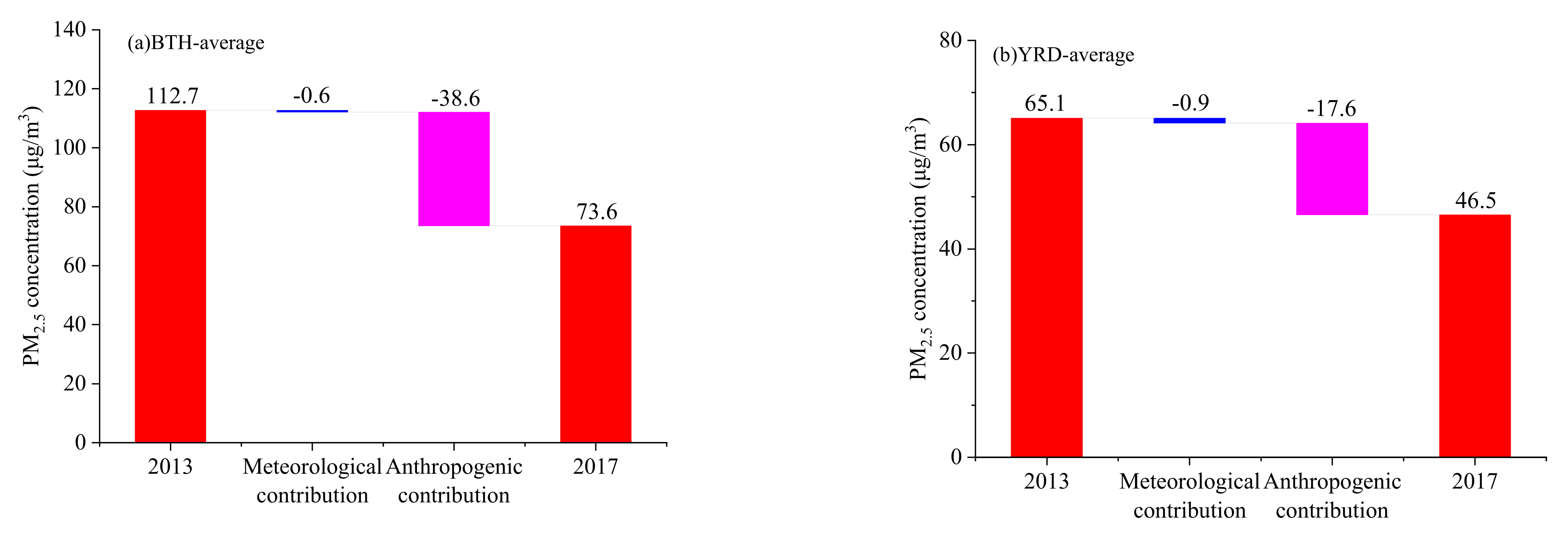
3.2. Impact of Meteorological Conditions and Anthropogenic Emissions during 2013–2017

3.2.1. Contribution from Changes in Meteorological Conditions

According to the single variable, the simulation results of the base cases E₁₇M₁₇ and the fixed meteorological sensitivity experiments E₁₇M_13–17 were compared to recognize the meteorological contribution during 2013–2017. That is, the higher the simulated concentration of PM_2.5 under different meteorological backgrounds, the worse the diffusion conditions of the corresponding meteorological year. Figure 5 shows the simulation results based on the same emission (2017) during the different meteorological years (from 2013 to 2017). From the simulated concentration, both the BTH and YRD regions have a similar variation in meteorological contribution, and the meteorological conditions in 2016 are more favorable than those in 2017, while in 2013–2015 they are unfavorable, especially 2015. The change in the meteorological contribution is consist with the [44] results. During 2013–2017, changes in the meteorological conditions contributed a 1.5 μg/m³ and 0.2 μg/m³ reduction in 2016, and a 1.6–3.8 μg/m³ and 1.1–3.6 μg/m³ increase from 2013 to 2015. Therefore, from the perspective of the variation trend of the inter-annual simulated concentration, the meteorological conditions are unfavorable in 2015 and are more favorable in 2016 than those in 2017.

Seasonal variations showed that the degree of meteorological contribution in BTH and YRD is slightly differently affected by the meteorological and climatic conditions in the small regional scale (as shown in Figure S1). Taking January as an example, the simulation concentrations of the BTH region were 130.0 and 118.1 μg/m³, respectively, and from 2013 to 2016, the meteorological contributions year by year were 11.9, 6.6, 6.7 and −4.2 μg/m³, respectively. While for the YRD regions, the simulation concentrations were 81.9 and 75.8 μg/m³, respectively, which are lower than those in the BTH region. The former four years’ contributions were 6.1, 5.5, 3.8 and 1.5 μg/m³, respectively. The results indicated that the meteorological conditions in January 2013 were more unfavorable than those in 2017 in the BTH and YRD regions, which is the main reason for the result of the 58.5% concentration increase for BTH and the 52.5% concentration increase for YRD PM_2.5. However, for April, the meteorological contributions had adverse tendencies, with the PM_2.5 concentration increasing to 3.7 and 1.3 μg/m³, respectively. Moreover, the favorable contributions were 6.9% and 2.9%, while the unfavorable contributions range was 0.2–9.4% and 0.2–9.3%. As for July, the meteorological conditions in different years had the same contribution variation as for April, so the meteorological conditions had a better diffusion in 2013 than in 2015. For October, the meteorological contribution had an opposite effect, with 1.6 μg/m³ for the BTH region and −0.8 μg/m³ for YRD. For the ratio of the meteorological contributions, the other three periods showed favorable meteorological conditions except for in 2014 in the BTH region, while in the YRD region, the meteorological kept being unfavorable from 2013 to 2015 in October and turned into favorable in 2016. Therefore, the variation characteristics of the meteorological conditions in the BTH and YRD regions basically kept the same favorable or unfavorable trends in the annual average variation, while in the monthly average variation there was no obvious consistency and there were even opposite characteristic changes in some periods.

3.2.2. Contribution from the Emission Reduction Measures

The simulated result of the base cases E₁₇M₁₇ and the fixed-emission sensitivity experiments E₁₇M₁₃, E₁₃M₁₃ and E₁₃M₁₇ could reflect the emission contributions in different years, since the PM_2.5 concentration was mainly affected by the meteorological changes and anthropogenic emissions. Assuming that all the contribution elements in the PM_2.5 concentration had a linear summation relationship, we normalized the meteorological changes and anthropogenic emission contributions based on the function in Section 2.5. Figure 6 shows the annual anthropogenic emission reduction contribution and the meteorological contribution in those two regions. Comparing the simulated and observed concentration in 2013, the emission and meteorological conditions led to a decrease of 36.8 and 2.4 μg/m³ in BTH, and 17.6 and 0.9 μg/m³ in the YRD region, respectively. The results proved that the PM_2.5 concentration could substantially reduce mainly owing to the anthropogenic emission reduction, while the meteorological conditions contribute less reduction than those in the former. By comparing the anthropogenic emission reduction ratio, the PM_2.5 has decreased by 51.6% in BTH and 63.9% in the YRD region, which led to the PM_2.5 concentration decreasing by 32.6% and 27.1%, respectively. Obviously, with the reduction in the emissions, the proportion of PM_2.5 concentration decrease in BTH was significantly higher than that in the YRD region. The reason for this was that the PM_2.5 concentration consisted with primary emission and secondary conversion, and the secondary conversion intensity would slow down followed by the primary emission reduction. However, when the PM_2.5 concentration reaches the corresponding threshold, the PM_2.5 concentration would decrease slowly by the emission reduction. Such anthropogenic contributions influencing the PM_2.5 in BTH and YRD have been reported in many previous studies [45].

Figure S2 shows the meteorological contribution and anthropogenic emission contribution in typical representative months. As for the order of the contribution intensities of the anthropogenic emission reduction, it was January (64.1 μg/m³) > October (44.7 μg/m³) > July (19.7 μg/m³) > October (18.5 μg/m³) in the BTH region, while for the YRD region, the order was January (30.4 μg/m³) > October (17.5 μg/m³) > April (15.5 μg/m³) > October (7.0 μg/m³). In terms of seasonal changes, affected by diffusion conditions and emission reduction, the proportion of anthropogenic emission reduction contributions was the highest in autumn and winter, both in the BTH region and YRD region. However, from the meteorological contribution aspect, the intensity varies from the season variation and it has a slightly different change. Taking January and October for examples, the meteorological conditions in the same month in 2013 were worse than those in 2017, with 11.9 and 6.1 μg/m³ for BTH and YRD in January, respectively, and 4.2 and 1.1 μg/m³ for the same regions in October, respectively. On the contrary, the meteorological conditions in April and July were better, which was of benefit for the diffusion of the pollutants, with −5.0 and −0.6 μg/m³ in BTH, and −3.2 and 0.8 μg/m³ in YRD, respectively. Therefore, for both the annual change and seasonal changes, the PM_2.5 concentration changes were mainly affected by the anthropogenic emission reduction, with a positive correlation and nonlinear. Moreover, it was obvious that the PM_2.5 concentration had a closer relationship to the reduction emission during the high PM_2.5 concentration period called “peak-down”.

3.2.3. Verified of Favorable and Unfavorable Condition in Meteorological

To analyze the meteorological influence, Typhoon Business and Service Regulations issued by the China Meteorological Bureau was introduced to verify the favorable and unfavorable conditions to the PM_2.5 concentration. According to the regulation, the wind level was divided into the following categories: no wind (0–0.2 m/s), soft wind (0.3–1.5 m/s), light wind (1.6–3.3 m/s), breeze wind (3.4–5.4 m/s), soft breeze (5.5–7.9 m/s), cool breeze (8.0–10.7 m/s) and strong wind (10.8–13.8 m/s), and the rest. The statistical analysis wind grade and relative humidity in the BTH and YRD regions are shown in Figure 7 and Figure S3. For January in the BTH region, the frequency of the no wind and soft wind are in the following order: 44.3% (2013) > 43.2% (2017) > 41.6% (2014) > 36.2% (2015) > 36.1% (2016), while the relative humidity in the corresponding wind grade order was 72.8% (2013) > 70.4% (2017) > 65.4% (2015) > 57.1% (2014) > 56.2% (2016). The results indicated that it was difficult to diffuse the pollution under low wind and high humidity and keep the same changes in the favorable and unfavorable years, and the meteorological conditions were unfavorable in 2013 and favorable in 2016 [46]. Conversely, the diffusion conditions with a high wind speed and low humidity have enhanced atmospheric turbulence to reduce the second transformation of pollutants. Similarly, in the YRD region, the frequency of the no wind and soft wind has the following order: 43.3% (2015) > 34.4% (2013) > 32.5% (2014) > 31.5% (2016)> 27.5% (2017), while the relative humidity in the corresponding wind grade order was 83.2% (2013) > 81.0% (2017) > 79.7% (2016) > 75.9% (2014) > 70.6% (2015). Compared to the BTH region, the relative humidity in the YRD region is higher. The reason is that there is a 3,461 km coastline in YRD, which is 5.5 times longer than that in BTH. Affected by the land and sea breeze, the clean air mass and vapor is easier to transfer to the inland areas. Thus, the air quality in YRD is better than that in the BTH region.

As for the other three months, the wind grade and humidity stayed the same with the meteorological favorable and unfavorable conditions. In terms of April, the sum of no wind and soft wind in 2015 was 1.7 times than that in 2017, while the relative humidity was 1.4 times in the same periods in the BTH region. However, in terms of the meteorological condition in 2013, the corresponding wind level was 0.6 times than that in 2017 with a 6.3% relative humidity gap. Thus, compared with the diffusion condition in the same month in 2017, the favorable year is 2013 while the unfavorable year is 2015, during 2013–2016. In July, the frequency of the same wind grades was 32.9% and 34.3%, and the relative humidity was 80.8% and 78.6%, respectively. In fact, the conditions of static stability were basically similar, but the high-wind with low-humidity conditions were slightly stronger than those in 2017, so the diffusion condition is better in April. For October, the total frequency of no wind and soft wind was as high as 53.9% and relative humidity was more than 70% in 2014, which led this year to be the worst in terms of its meteorological condition. As for the YRD region, the relative humidity and wind grade were consistent with the same law of the diffusion condition.

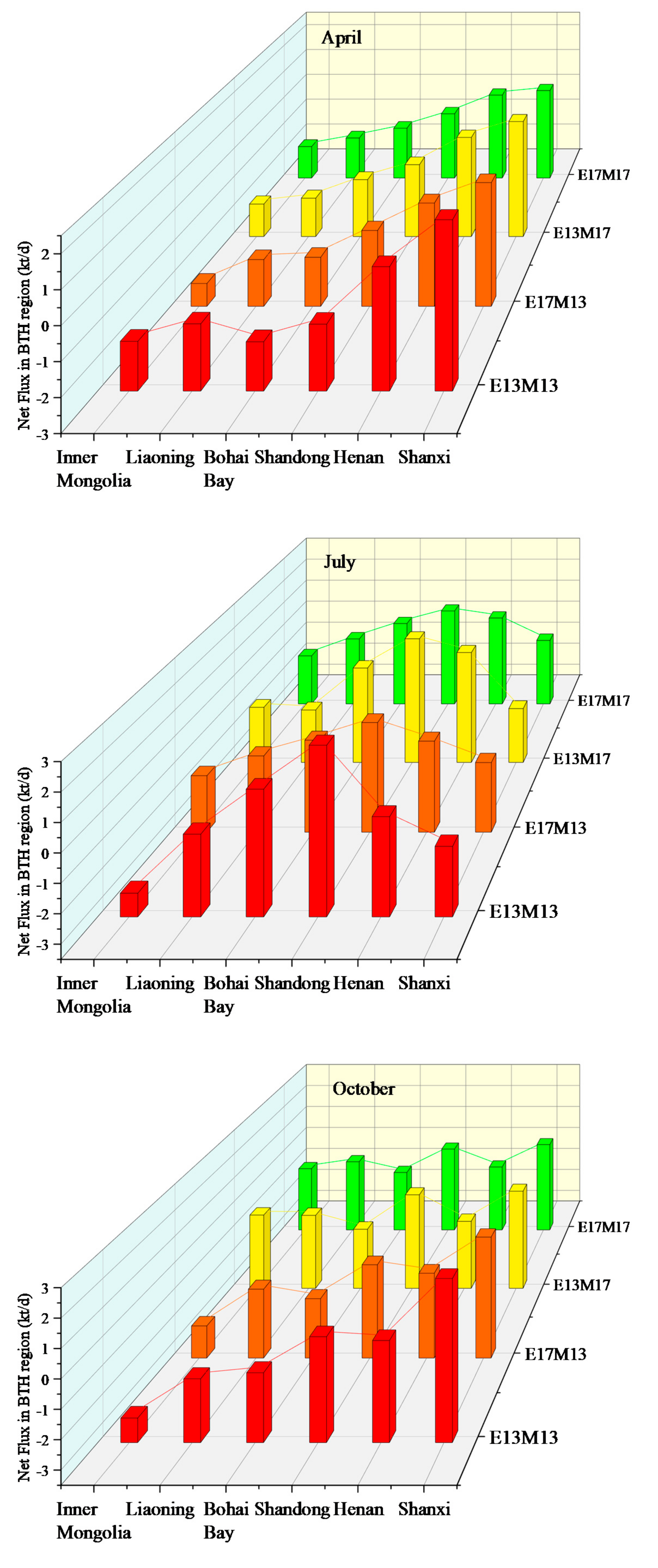
3.3. Transport Flux among the BTH and YRD Regions

Figure 8 shows the inflow, outflow and net flux of the PM_2.5 seasonal changes in 2017, from the surface to the height of 1800 m from the ground. In general, the inflow and outflow fluxes have seasonal variation, and the inflow flux intensities are as follows: January (14.1 kt/d) > April (7.5 kt/d) > July (7.3 kt/d) > October (6.1 kt/d). The outflow intensities are as follows: January (−12.3 kt/d) > April (−11.8 kt/d) > July (−8.4 kt/d) > October (−8.1 kt/d). The highest value of inflow flux and outflow flux were 2.3 times and 1.5 times of the lowest value, respectively. In January, April and October, the BTH region was greatly affected by the Shanxi province with net fluxes of 3.1, 0.4 and 0.4 kt/d, respectively. For July, the BTH region was greatly affected by the Shandong province with a net flux of 0.7 kt/d. As for the outflow intensity, the BTH region was mainly exported to Liaoning and Bohai Bay in January, Inner Mongolia and Shanxi in April and October, and Inner Mongolia and Bohai Bay in July. The absolute value of the PM_2.5 net flux is in the following order: April (4.3 kt/d) > October (2.0 kt/d) > January (1.7 kt/d) > July (1.2 kt/d). In general, the BTH region served as a “sink” in January and played the role of a “source” in the other months. With the influence of inflow and outflow fluxes, we recognized the various PM_2.5 transport pathways in the two regions during the four months. There were one or two key transport pathways, as follows: Shanxi → BTH → Liaoning and Inner Mongolia → BTH → Bohai Bay in January, Shanxi and Henan → BTH → Inner Mongolia and Bohai Bay in April, Shandong → BTH → Shanxi and Inner Mongolia and Henan → BTH → Liaoning in July, and Shanxi → BTH → Bohai Bay and Shandong → BTH → Inner Mongolia. It noted that all the transport paths were affected by the monsoon circulation change.

To investigate the vertical variations with different altitudes in net flux across the region, and clearly make the chief transport height layers, we calculated the distribution of the monthly net flux in four months, as shown in Figure 9. In January, BTH acted as a “convergence” in ~132 m and 817–1782 m with the inflow flux ranging from 32.6 to 564.8 t/d from the Shanxi and Inner Mongolia, and the outflow flux ranging from −16.0 to −225.7 t/d toward Shandong and Bohai Bay. In the range of 252–611 m, BTH turned to a “source” role, which mainly transported toward Bohai Bay as −2.9 to −157.7 t/d. It noted that the wind field condition at the boundary between BTH and Bohai Bay had increased significantly with the increase in the height. In April, the BTH region appeared as a “source” at different heights from the ground. The net outflow flux reached the maximum intensity, reaching −548.7 t/d at 817 m. Different from April, the strongest intensity occurred at 1782 m with a −296.6 t/d outflow magnitude, and the dominated contributor areas turned from Shandong to Shanxi. For October, the BTH region still behaved as a “source”, Henan and Inner Mongolia were the areas mainly receiving the outflow, which ranged from −29.1 to 104.0 t/d.

3.4. Impact of Meteorological Parameters and Anthropology Emission on the Transport Net Flux during 2013–2017

3.4.1. Impact of Anthropology Emission on the Transport Net Flux during 2013–2017

Based on the E₁₇M₁₃, E₁₇M₁₇, E₁₃M₁₃ and E₁₃M₁₇ four scenarios, we calculated the corresponding net transport flux on the BTH region, as shown in Figure 10. Taking the BTH region for example, the inflow flux, outflow flux and net flux intensity in E₁₃M₁₇ were 1.19–1.49, 1.21–1.42, and 1.02–1.85 times than those in the E₁₇M₁₇ scenario, respectively. As for the main transport paths, there were still two paths, Shanxi → BTH → Liaoning and Inner Mongolia → BTH → Bohai Bay and Shandong. It noted that with the reduction in emission, the inflow and outflow fluxes also appeared downward, with the strongest decline inflow magnitude occurring in Henan and the strongest decline outflow magnitude occurring in Shandong. During 2013–2017, the adjacent cities around the BTH region implemented a number of pollution mitigation measures, there is a positive correlation between the concentration of PM_2.5 and the amount of emission. In addition, the results of the total net inflow flux in January showed that with the reduction in emissions, the intensity of the inflow flux reduction was lower than the outflow flux intensity, which is one of the mainly reasons for the increase in the local pollutant concentrations. Judging from the changes in the other months, the characteristics of the multiple changes are basically the same as in January. It is worth noting that the total net flux intensity value has declined in some provinces. For example, Shandong and Bohai Bay in April, and Inner Mongolia in July and October have different degrees of decline in the total net flux. This phenomenon was caused by the different changes in the inflow and outflow flux, which further proved that there is a non-linear relationship between the pollutant concentration and emission. The change pattern of E₁₃M₁₃ and E₁₃M₁₇ is basically consistent with the comparison results of the above former scenarios.

For the YRD region, the inflow flux, outflow flux and net flux intensity of E₁₃M₁₇ were 1.26–1.87, 1.12–1.37 and 0.54–1.35 times than the flux intensity under the scenario E₁₇M₁₇, respectively (as shown in Figure S4). Compared with the BTH region, both the regions have adjacent sea areas, but the coastline of the former is much smaller than the latter. The Shandong and Henan provinces, as the connect areas for both the BTH and YRD regions, have significant transmission effects on those two regions but the total net flux direction is opposite. In winter, affected by prevail zonal circulation and northwest airflow, northwest wind prevails over most parts of our country. Located downwind of Shandong and Henan, the YRD region gradually takes on a “convergence” role. From the change patterns of the other months, the inflow fluxes in April, July and October varied from 1.15–1.88 times, 1.30–2.16 times and 1.21–1.58 times, and the outflow flux varied from 1.18–1.77, 1.42–2.12 and 1.09–1.40 times, respectively. Similarly, the total net flux intensity value of the East Sea, Jiangxi, Hubei and Henan also declined in some provinces in January. Different from the BTH region, the YRD region is represented as having a “source” role, while the BTH region turned shift among the “source” and “convergence” roles.

3.4.2. Impact of Meteorological Changes on the Transport Net Flux during 2013–2017

Based on the E₁₇M_13~17 five scenarios, we calculated the corresponding net transport flux on the BTH and YRD regions, as shown in Figure 11 and Figure S5. Under different meteorological conditions, it is found that the contribution of meteorological factor disturbance to the flux change is slightly lower than that of anthropogenic emissions, and the inflow or outflow flux also has an opposite trend, which is due to the meteorological factor disturbance. Meteorological factor disturbances mainly include multiple factors such as changes in the wind speed intensity at the boundary line, changes in the relative humidity, and changes in the height of the mixed boundary layer. The response of each element to changes in pollutant concentration is complex. The calculation results use the boundary line to extract the corresponding grid flux change, which is susceptible to a sudden decrease and sharp rise in the concentration of the small area-scale meteorological field change. In addition, the flux is the pollutant concentration and the wind field vector product, so the flux change intensity is not exactly the same. The total net inflow flux and the total net outflow flux intensity are opposite to the meteorological favorable and unfavorable degree changes, that is, when the total net flux is inflow, the more favorable the meteorological conditions are, and the lower the net inflow flux intensity. Conversely, when the total net flux is outflow, the more favorable the meteorological conditions are, and the higher the net outflow flux intensity. The main transmission path is not subject to changes in weather conditions, but the strength of the dominant transmission path changes during certain periods. Similarly, in the YRD region, it is also found that the significance of the disturbance of meteorological factors to the flux change is slightly lower than the contribution of the anthropogenic emission change, and the inflow or outflow flux also has an opposite trend. The results of the inter-annual variation also show that when the total net flux is outflow, the more favorable the meteorological conditions are.

4. Conclusions

We conducted a comprehensive analysis of the decrease in the annual average PM_2.5 concentration in the BTH and YRD regions from 2013 to 2017. Based on the PM_2.5 concentration and wind vector, the corresponding surface and vertical transport flux intensities were calculated. Then, based on a set of simulation scenarios and decomposed attribution analyses, the emission reduction and meteorological condition were estimated on the PM_2.5 concentration and transport fluxes. The primary conclusions are summarized as follows.

The average mass concentrations of PM_2.5 were 105.9 ± 51.7 μg/m³ for BTH, 67.8 ± 28.2 μg/m³ for YRD in 2013, respectively. Follow by the descend rate, PM_2.5 had the second greatest decrement of −39.58% in BTH and −28.07% in YRD, which overfulfilled the Air Pollution Prevention and Control Action Plan (APPCAP) target. Moreover, the two target regions average PM_2.5 in each month had a huge decline by more than 20% in BTH and 15% in YRD.

According to the simulation experiments and decomposed attribution analyses, the favorable and unfavorable meteorological conditions were selected by the simulation concentration. Both the BTH and YRD regions kept a similar variation from the meteorological contribution, and the meteorological conditions in 2016 were more favorable than those in 2017 while 2013–2015 was unfavorable, especially 2015. Affected by the meteorological and climatic conditions in the small regional scale, it is slightly different for the degree of meteorological contribution in BTH and YRD. By normalized meteorological changes and anthropogenic emission contributions, the emission and meteorological conditions led to a decrease of 36.8 and 2.4 μg/m³ in BTH and 17.6 and 0.9 μg/m³ in the YRD region.

The influence of anthropogenic emissions on the transmission flux is as follows: The inflow flux, outflow flux, and net flux vary with the intensity of anthropogenic emissions, but the magnitude of the change is slightly different. The net flux has no obvious change rule with the increase in the intensity; the change in the emission intensity has no obvious change on the main transmission path, but only affects the absolute value of the flux change under the transmission path; with the increase in the emission intensity, the total cross-border flux increased. The net inflow flux increased significantly, and the total net outflow flux decreased significantly.

The influence of meteorological contribution on the transmission flux was as follows: The inflow flux, the outflow flux, and the net flux change with the change in meteorological contribution, but the variation range is obviously different; under the favorable meteorological background, the total net inflow flux shows a significant decrease, the net outflow flux increases significantly, and the absolute value of the decrease/increase intensity is positively correlated with the degree of favorable/unfavorable weather; the change in meteorological contribution has no obvious change on the main transmission path, and only affects the transmission path.

References

1. Li, H.Y.; Zhang, Q.; Zheng, B.; Chen, C.R.; Wu, N.N.; Guo, H.Y.; Zhang, Y.X.; Zheng, Y.X.; Li, X.; He, K.B. Nitrate-driven urban haze pollution during summertime over the North China Plain. Atmos. Chem. Phys. 2018, 18, 5293–5306. [Google Scholar] [CrossRef] [Green Version]
2. Wang, G.; Deng, J.; Zhang, Y.; Zhang, Q.; Jiang, J. Air pollutant emissions from coal-fired power plants in China over the past two decades. Sci. Total Environ. 2020, 741, 140326. [Google Scholar] [CrossRef]
3. Qi, M.; Zhu, X.; Du, W.; Chen, Y.; Chen, Y.; Huang, T.; Pan, X.; Zhong, Q.; Sun, X.; Zeng, E.Y. Exposure and health impact evaluation based on simultaneous measurement of indoor and ambient PM2.5 in Haidian, Beijing. Environ. Pollut. 2016, 220, 704–712. [Google Scholar] [CrossRef] [PubMed]
4. Zhang, H.; Cheng, S.; Li, J.; Yao, S.; Wang, X. Investigating the aerosol mass and chemical components characteristics and feedback effects on the meteorological factors in the Beijing-Tianjin-Hebei region, China. Environ. Pollut. 2019, 244, 495–502. [Google Scholar] [CrossRef] [PubMed]
5. Zheng, Y.; Xue, T.; Zhang, Q.; Geng, G.; Tong, D.; Li, X.; He, K. Air quality improvements and health benefits from China’s clean air action since 2013. Environ. Res. Lett. 2017, 12, 114020. [Google Scholar] [CrossRef]
6. Zhu, X.; Che, Z.; Cao, J.; Liu, Y.; Yao, C. Maternal exposure to fine particulate matter PM2.5 and pregnancy outcomes: A meta-analysis. Environ. Sci. Pollut. Res. 2015, 22, 3383. [Google Scholar] [CrossRef] [PubMed]
7. Han, L.; Xiang, X.; Zhang, H.; Cheng, S.; Wang, H.; Wei, W.; Wang, H.; Lang, J. Insights into submicron particulate evolution, sources and influences on haze pollution in Beijing, China. Atmos. Environ. 2019, 201, 360–368. [Google Scholar] [CrossRef]
8. Song, X.; Yang, S.; Shao, L.; Fan, J.; Liu, Y. PM10 mass concentration, chemical composition, and sources in the typical coal-dominated industrial city of Pingdingshan, China. Sci. Total Environ. 2016, 571, 1155–1163. [Google Scholar] [CrossRef]
9. Cheng, Z.; Wang, S.; Jiang, J.; Fu, Q.; Chen, C.; Xu, B.; Yu, J.; Fu, X.; Hao, J. Long-term trend of haze pollution and impact of particulate matter in the Yangtze River Delta, China. Environ. Pollut. 2013, 182, 101–110. [Google Scholar] [CrossRef]
10. Wang, Y.; Li, W.; Gao, W.; Liu, Z.; Tian, S.; Shen, R.; Ji, D.; Wang, S.; Wang, L.; Tang, G.; et al. Trends in particulate matter and its chemical compositions in China from 2013-2017. Sci. China-Earth Sci. 2019, 62, 1857–1871. [Google Scholar] [CrossRef]
11. Shu, L.; Wang, T.; Han, H.; Xie, M.; Chen, P.; Li, M.; Wu, H. Summertime ozone pollution in the Yangtze River Delta of eastern China during 2013-2017: Synoptic impacts and source apportionment. Environ. Pollut. 2020, 257, 113631. [Google Scholar] [CrossRef] [PubMed]
12. Liu, T.; Gong, S.; He, J.; Yu, M.; Wang, Q.; Li, H.; Liu, W.; Zhang, J.; Li, L.; Wang, X.; et al. Attributions of meteorological and emission factors to the 2015 winter severe haze pollution episodes in China’s Jing-Jin-Ji area. Atmos. Chem. Phys. 2017, 17, 2971–2980. [Google Scholar] [CrossRef] [Green Version]
13. Cai, S.; Wang, Y.; Zhao, B.; Wang, S.; Chang, X.; Hao, J. The impact of the “Air Pollution Prevention and Control Action Plan” on PM2.5 concentrations in Jing-Jin-Ji region during 2012–2020. Sci. Total Environ. 2017, 580, 197–209. [Google Scholar] [CrossRef] [PubMed]
14. Zhao, B.; Wang, S.; Wang, J.; Fu, J.S.; Liu, T.; Xu, J.; Fu, X.; Hao, J. Impact of national NOx and SO2 control policies on particulate matter pollution in China. Atmos. Environ. 2013, 77, 453–463. [Google Scholar] [CrossRef]
15. Wang, Y.; Bao, S.; Wang, S.; Hu, Y.; Shi, X.; Wang, J.; Zhao, B.; Jiang, J.; Zheng, M.; Wu, M.; et al. Local and regional contributions to fine particulate matter in Beijing during heavy haze episodes. Sci. Total Environ. 2017, 580, 283–296. [Google Scholar] [CrossRef]
16. Chen, Z.; Xie, X.; Cai, J.; Chen, D.; Gao, B.; He, B.; Cheng, N.; Xu, B. Understanding meteorological influences on PM2.5 concentrations across China: A temporal and spatial perspective. Atmos. Chem. Phys. 2018, 18, 5343–5358. [Google Scholar] [CrossRef] [Green Version]
17. Zhang, H.; Xing, Y.; Cheng, S.; Wang, X.; Guan, P. Characterization of multiple atmospheric pollutants during haze and non-haze episodes in Beijing, China: Concentration, chemical components and transport flux variations. Atmos. Environ. 2021, 246, 118129. [Google Scholar] [CrossRef]
18. Hong, Y.; Xu, X.; Liao, D.; Ji, X.; Hong, Z.; Chen, Y.; Xu, L.; Li, M.; Wang, H.; Zhang, H.; et al. Air pollution increases human health risks of PM2.5-bound PAHs and nitro-PAHs in the Yangtze River Delta, China. Sci. Total Environ. 2021, 770, 145402. [Google Scholar] [CrossRef]
19. Cheng, J.; Su, J.; Cui, T.; Li, X.; Dong, X.; Sun, F.; Yang, Y.; Tong, D.; Zheng, Y.; Li, Y.; et al. Dominant role of emission reduction in PM2.5 air quality improvement in Beijing during 2013–2017: A model-based decomposition analysis. Atmos. Chem. Phys. 2019, 19, 6125–6146. [Google Scholar] [CrossRef] [Green Version]
20. Zhang, X.; Zhong, J.; Wang, J.; Wang, Y.; Liu, Y. The interdecadal worsening of weather conditions affecting aerosol pollution in the Beijing area in relation to climate warming. Atmos. Chem. Phys. 2018, 18, 5991–5999. [Google Scholar] [CrossRef] [Green Version]
21. Zhao, B.; Jiang, J.H.; Gu, Y.; Diner, D.; Worden, J.; Liou, K.-N.; Su, H.; Xing, J.; Garay, M.; Huang, L. Decadal-scale trends in regional aerosol particle properties and their linkage to emission changes. Environ. Res. Lett. 2017, 12, 054021. [Google Scholar] [CrossRef]
22. Liu, F.; Zhang, Q.; van der A Ronald, J.; Zheng, B.; Tong, D.; Yan, L.; Zheng, Y.; He, K. Recent reduction in NOx emissions over China: Synthesis of satellite observations and emission inventories. Environ. Res. Lett. 2016, 11, 114002. [Google Scholar] [CrossRef] [Green Version]
23. Zeng, J.; Wang, M.-E.; Zhang, H.-X. Correlation between atmospheric PM2.5 concentration and meteorological factors during summer and autumn in Beijing, China. J. Appl. Ecol. 2014, 25, 2695–2699. [Google Scholar]
24. Ma, Q.; Wu, Y.; Zhang, D.; Wang, X.; Xia, Y.; Liu, X.; Tian, P.; Han, Z.; Xia, X.; Wang, Y.; et al. Roles of regional transport and heterogeneous reactions in the PM2.5 increase during winter haze episodes in Beijing. Sci. Total Environ. 2017, 599, 246–253. [Google Scholar] [CrossRef]
25. Zhang, Y.L.; Cao, F. Fine particulate matter PM2.5 in China at a city level. Sci. Rep. 2015, 5, 14884. [Google Scholar] [CrossRef] [Green Version]
26. Wang, X.; Wei, W.; Cheng, S. Composition analysis and formation pathway comparison of PM1 between two pollution episodes during February 2017 in Beijing, China. Atmos. Environ. 2020, 223, 117223. [Google Scholar] [CrossRef]
27. Guan, P.; Wang, X.; Cheng, S.; Zhang, H. Temporal and spatial characteristics of PM2.5 transport fluxes of typical inland and coastal cities in China. J. Environ. Sci. 2021, 103, 229–245. [Google Scholar] [CrossRef]
28. Jia, J.; Cheng, S.; Yao, S.; Xu, T.; Zhang, T.; Ma, Y.; Wang, H.; Duan, W. Emission characteristics and chemical components of size-segregated particulate matter in iron and steel industry. Atmos. Environ. 2018, 182, 115–127. [Google Scholar] [CrossRef]
29. Zhou, Y.; Cheng, S.Y.; Lang, J.L.; Chen, D.S.; Zhao, B.B.; Liu, C.; Xu, R.; Li, T.T. A comprehensive ammonia emission inventory with high-resolution and its evaluation in the Beijing-Tianjin-Hebei (BTH) region, China. Atmos. Environ. 2015, 106, 305–317. [Google Scholar] [CrossRef]
30. Sun, X.W.; Cheng, S.Y.; Lang, J.L.; Ren, Z.H.; Sun, C. Development of emissions inventory and identification of sources for priority control in the middle reaches of Yangtze River Urban Agglomerations. Sci. Total Environ. 2018, 625, 155–167. [Google Scholar] [CrossRef]
31. Li, M.; Zhang, Q.; Zheng, B.; Tong, D.; Lei, Y.; Liu, F.; Hong, C.P.; Kang, S.C.; Yan, L.; Zhang, Y.X.; et al. Persistent growth of anthropogenic non-methane volatile organic compound (NMVOC) emissions in China during 1990-2017: Drivers, speciation and ozone formation potential. Atmos. Chem. Phys. 2019, 19, 8897–8913. [Google Scholar] [CrossRef] [Green Version]
32. Zheng, B.; Tong, D.; Li, M.; Liu, F.; Hong, C.P.; Geng, G.N.; Li, H.Y.; Li, X.; Peng, L.Q.; Qi, J.; et al. Trends in China’s anthropogenic emissions since 2010 as the consequence of clean air actions. Atmos. Chem. Phys. 2018, 18, 14095–14111. [Google Scholar] [CrossRef] [Green Version]
33. Zhou, Y.; Cheng, S.Y.; Chen, D.S.; Lang, J.L.; Zhao, B.B.; Wei, W. A new statistical approach for establishing high-resolution emission inventory of primary gaseous air pollutants. Atmos. Environ. 2014, 94, 392–401. [Google Scholar] [CrossRef]
34. Xing, X.F.; Zhou, Y.; Lang, J.L.; Chen, D.S.; Cheng, S.Y.; Han, L.H.; Huang, D.W.; Zhang, Y.Y. Spatiotemporal variation of domestic biomass burning emissions in rural China based on a new estimation of fuel consumption. Sci. Total Environ. 2018, 626, 274–286. [Google Scholar] [CrossRef]
35. Li, Y.; Ye, C.; Liu, J.; Zhu, Y.; Wang, J.; Tan, Z.; Lin, W.; Zeng, L.; Zhu, T. Observation of regional air pollutant transport between the megacity Beijing and the North China Plain. Atmos. Chem. Phys. 2016, 16, 14265–14283. [Google Scholar] [CrossRef] [Green Version]
36. Liu, F.; Zhang, Q.; Tong, D.; Zheng, B.; Li, M.; Huo, H.; He, K.B. High-resolution inventory of technologies, activities, and emissions of coal-fired power plants in China from 1990 to 2010. Atmos. Chem. Phys. 2015, 15, 13299–13317. [Google Scholar] [CrossRef] [Green Version]
37. Wang, L.; Wei, Z.; Wei, W.; Fu, J.S.; Meng, C.; Ma, S. Source apportionment of PM2.5 in top polluted cities in Hebei, China using the CMAQ model. Atmos. Environ. 2015, 122, 723–736. [Google Scholar] [CrossRef]
38. Zhao, B.; Wang, S.; Donahue, N.M.; Jathar, S.H.; Huang, X.; Wu, W.; Hao, J.; Robinson, A.L. Quantifying the effect of organic aerosol aging and intermediate-volatility emissions on regional-scale aerosol pollution in China. Sci. Rep. 2016, 6, 28815. [Google Scholar] [CrossRef] [Green Version]
39. Li, J.; Han, Z. A modeling study of severe winter haze events in Beijing and its neighboring regions. Atmos. Res. 2016, 170, 87–97. [Google Scholar] [CrossRef]
40. Chang, X.; Wang, S.; Zhao, B.; Cai, S.; Hao, J. Assessment of inter-city transport of particulate matter in the Beijing-Tianjin-Hebei region. Atmos. Chem. Phys. 2018, 18, 4843–4858. [Google Scholar] [CrossRef]
41. Jiang, C.; Wang, H.; Zhao, T.; Li, T.; Che, H. Modeling study of PM2.5 pollutant transport across cities in China’s Jing-Jin-Ji region during a severe haze episode in December 2013. Atmos. Chem. Phys. 2015, 15, 5803–5814. [Google Scholar] [CrossRef] [Green Version]
42. Zhai, S.; Jacob, D.J.; Wang, X.; Shen, L.; Li, K.; Zhang, Y.; Gui, K.; Zhao, T.; Liao, H. Fine particulate matter PM2.5 trends in China, 2013–2018: Separating contributions from anthropogenic emissions and meteorology. Atmos. Chem. Phys. 2019, 19, 11031–11041. [Google Scholar] [CrossRef] [Green Version]
43. Zhang, Y.; Dore, A.J.; Ma, L.; Liu, X.J.; Ma, W.Q.; Cape, J.N.; Zhang, F.S. Agricultural ammonia emissions inventory and spatial distribution in the North China Plain. Environ. Pollut. 2010, 158, 490–501. [Google Scholar] [CrossRef] [Green Version]
44. Zhang, Q.; Zheng, Y.X.; Tong, D.; Shao, M.; Wang, S.X.; Zhang, Y.H.; Xu, X.D.; Wang, J.N.; He, H.; Liu, W.Q.; et al. Drivers of improved PM2.5 air quality in China from 2013 to 2017. Proc. Natl. Acad. Sci. USA 2019, 116, 24463–24469. [Google Scholar] [CrossRef] [Green Version]
45. Huang, C.H.; Liu, K.; Zhou, L. Spatio-temporal trends and influencing factors of PM2.5 concentrations in urban agglomerations in China between 2000 and 2016. Environ. Sci. Pollut. Res. 2021, 28, 10988–11000. [Google Scholar] [CrossRef]
46. Li, Y.; Liao, Q.; Zhao, X.; Tao, Y.; Bai, Y.; Peng, L. Premature mortality attributable to PM2.5 pollution in China during 2008-2016: Underlying causes and responses to emission reductions. Chemosphere 2021, 263, 127925. [Google Scholar] [CrossRef]
Figure 1. Double-nesting domains performed in the CAMx simulation.
Sustainability 13 05685 g001
Figure 2. Comparison of observed (red) and CAMx-simulated (black) daily mean PM2.5 concentration over Beijing (a1), Tianjin (a2), Shijiazhuang (a3) (for BTH region) and Shanghai (a4), Hangzhou (a5), Nanjing (a6) (for YRD region) in 2013.
Sustainability 13 05685 g002
Figure 3. Comparison of the simulation and observations of PM2.5 compositions, concentration values are all reported in μg/m3.
Sustainability 13 05685 g003
Figure 4. Observed monthly (a1 for BTH and b1 for YRD) and annual (a2 for BTH and b2 for YRD) average PM2.5 in BTH and YRD during 2013–2017.
Sustainability 13 05685 g004
Figure 5. Relative contribution concentration of meteorological conditions changes (red lines is deviation value and boxes is concentration in the relationship year) in 2017 and a typical month in BTH (a) and YRD (b) regions.
Sustainability 13 05685 g005
Figure 6. The anthropogenic and meteorological contribution of PM2.5 in typical months in BTH (a) and YRD (b) regions.
Sustainability 13 05685 g006
Figure 7. Distribution of downwind frequency and relative humidity of different grades in different years in BTH region.
Sustainability 13 05685 g007
Figure 8. Seasonal variation in transport flux intensity between BTH region and neighboring provinces in 2017.
Sustainability 13 05685 g008
Figure 9. The net PM2.5 flux in the BTH region and its surrounding regions in 2017 was vertically distributed.
Sustainability 13 05685 g009
Figure 10. The characteristics of net flux of a typical month under different anthropogenic scenarios in BTH region.
Sustainability 13 05685 g010aSustainability 13 05685 g010b
Figure 11. The characteristics of net flux of a typical month under different meteorological scenarios in BTH region.
Sustainability 13 05685 g011aSustainability 13 05685 g011b