Forecasting of Disassembly Waste Generation under Uncertainties Using Digital Twinning-Based Hidden Markov Model

Abstract

Disassembly waste generation forecasting is the foundation for determining disassembly waste treatment and process formulation and is also an important prerequisite for optimizing waste management. The prediction of disassembly waste generation is a complex process which is affected by potential time, environment, and economy characteristic variables. Uncertainty features, such as disassembly amount, disassembly component status, and workshop scheduling, play an important role in predicting the fluctuation of disassembly waste generation. We therefore focus on revealing the trend of waste generation in disassembly remanufacturing that faces significant influences of technology and economic changes to achieve circular industry sustainable development. To dynamically predict the generation of disassembly waste under uncertainty, this work proposes a statistical method driven by a probabilistic model, which integrates the digital twinning, Gaussian mixture, and the hidden Markov model (DG-HMM). First, digital twinning technology is used for real-time data interaction between simulation prediction and decision evaluation. Then, the Gaussian mixture and HMM are used to dynamically predict the generation of disassembly waste. In order to effectively predict the amount of disassembly waste generation, real data collected from a disassembly enterprise are used to train and verify the model. Finally, the proposed model is compared with other general prediction models to illustrate the correctness and feasibility of the proposed model. The comparison results show that DG-HMM has better prediction accuracy for the actual disassembly waste generation.

1. Introduction

With the shortening of product life cycle and the acceleration of product upgrade, the rapid growth of obsolete products will put tremendous pressure on the ecological environment and human health [1,2]. The development of environmental awareness and the circular economy has forced manufacturers to increasingly consider the importance of environment protection in the production process [3]. Effective treatment of disassembly waste has become an important factor in the industrial circular economy and sustainable industrial development [4]. Disassembly waste is the useless solid, semi-solid and oil–water mixture produced in dismantling activities, including rust and nonferrous metals (cadmium, chromium, mercury, etc.), batteries, plastics, and various working fluids (lubricants, engine oil, etc.) [5]. Random dumping or improper disposal of disassembly waste can seriously endanger human health and even cause damage to the ecological environment. The prediction of disassembly waste generation is a complex process, which is affected by many factors, including rapid product upgrades, new technological innovations, machine usage conditions, component damage, and storage time. These influential factors in waste generation and their uncertainties are difficult to quantify [6]. Therefore, how to predict the generation of dismantling waste in an uncertain environment has become full of challenges. On this basis, in order to promote the sustainable development of resources, the ecosystem, and the environment [7,8], it is of great significance to study disassembly waste in the industrial system.

The existing approaches for waste generation forecasting are classified into four main categories: traditional statistical models [9,10], the gray and fuzzy models [11], simulation models [12], and nonprobabilistic statistical learning models [13]. In terms of traditional statistical models, Karpušenkaitė [14], Box [15], Giannouli [16], Chen [17], Althaf [18], and others have studied the time series prediction of uni-variate models involving environmental applications. Denafas [19] applied the municipal waste composition data to a time series prediction model, which can quantitatively estimate seasonally changing waste generation. Unlike deterministic models, stochastic models and probabilistic model-driven statistical methods have been widely used to predict waste generation under uncertain conditions [20,21], for example, by Peeters [22], Karpušenkaitė [23], Abdoli [24], and Kannangara [25]. However, the uncertainties about input data and predicted recovery potential are often overlooked. Gray and fuzzy theories can solve the problem of uncertainty [26], and a reliable model output can be obtained even with poor data. Chauhan [27] integrated interpretive structure modeling, a fuzzy analytic hierarchy process, and fuzzy technology to predict medical waste with order preference. Noori [28] combined a wavelet transform fuzzy system and a wavelet transform artificial neural network to predict solid waste generation. At the same time, with the increasing requirements for green sustainable development and cleaner production management technology [29,30], in terms of the current research situation, Tsai [31], Roubík [32], and Ahamed [33] have conducted extensive research on waste resource reuse, environmental climate change, and waste system management. Bai [34] presented an overview of the current solid waste management situation in Singapore and provided a brief discussion of the future challenges.

However, most of the mainstream studies focused on the dynamic prediction of waste generation in a certain time period or system, lacking research on the real-time dynamic prediction of waste generation under uncertainty [35]. Therefore, in this study, based on the HMM prediction model [36], we make improvements to be suitable for real-time dynamic prediction of dismantling waste. During the disassembly process, a lot of data about disassembly waste will be generated. In order to improve the accuracy of prediction, it is necessary to introduce digital twinning to dynamically predict the generation of disassembly waste. In addition, Gaussian mixture regression (GMR) constructs the joint probability density function of data and obtains a regression function from the probability model. The density estimation can reflect the trend of most data, which is an advantage for the prediction of dismantling waste. In this work, digital twinning technology, Gaussian mixture, and hidden Markov model (DG-HMM) are integrated to solve the interference factors of dynamic prediction. The proposed model is a new solution for the waste generation prediction in the disassembly process.

The primary objective of this paper is to dynamically predict in real-time the generation of disassembly waste, so as to provide necessary references for waste management, production technical improvement, and the capital budget of the disassembly system. Therefore, the contributions of this paper are mainly in three points: (1) A novel DG-HMM, which integrates digital twinning, Gaussian mixture, and HMM, was proposed to dynamically predict in real-time disassembly waste generation under uncertainty. (2) Based on the prediction model of HMM, the wavelet denoising was used for data cleaning, and a weighted average Gaussian mixture method was suggested to solve the problem of disassembly waste generation. (3) The proposed DG-HMM forecasting framework, including data pretreatment and forecasting analysis, can be expressed in an HMM to reduce prediction uncertainty. The proposed model was applied to a real case using daily disassembly waste generation data from 1 January 2018 to 31 December 2018, and its reliability and accuracy in forecast were verified.

2. Problem Description and Modeling

2.1. DG-HMM Modeling

In this model, the uncertainty of disassembly waste was a hidden variable. It is assumed that the hidden state sequence follows discrete time and a first-order Markov chain, which means that the current state only depends on the previous state. The predictor variable is regarded as an observation of a continuous random variable. In this work, we assumed that the observation was conditionally independent of generated states. The hidden state sequence was composed of the total uncertainty of disassembly waste generation, and the observation sequence was composed of actual values. The generation of disassembly waste is a noncyclical fluctuation problem.

DG-HMM includes two main stages, namely the dynamic prediction and the decision evaluation. In the dynamic prediction stage, the wavelet denoising is a tool for removing noise in the data series, and then HMM is used for forecasting. When the prediction accuracy exceeds the given value, the prediction result will enter the decision evaluation stage. In the decision evaluation stage, the algorithm parameters are reset, the model is trained, then Gaussian mixture mutation is used, and finally training data are postprocessed. The predicted values that satisfy the prediction accuracy requirements will be output to physical workshop. Real-time data interaction can be carried out between dynamic prediction and decision evaluation. The data of each forecast will be automatically saved in the database so that they can be used in parameter setting and decision making for the next forecast. The prediction results of the model can provide a theoretical reference for disassembly waste generation and planning implementation. The structure of the DG-HMM dynamic prediction of disassembly waste generation is shown in Figure 1.

In HMM, $z_t$ represents the discrete time of a hidden state at time t, $0\le t\le T,$ and $x_t$ represents the observation sequence. The conditional distribution of an observed state is $p(x_t|z_t).$ The probability of $z_t$ is related to the state of $z_{t-1}$. The latent variables can be expressed as k-dimensional binary variables. The transition probability matrix corresponds to a number table, which is represented by A:

$$A=\left[\begin{array}{ccc}{a}_{11}& L& a_{1K}\\ M& 0& M\\ a_{K1}& L& a_{KK}\end{array}\right]$$

(1)

where $a_{ij}$ is the transition probability from state i to state j, $a_{ij}=p\left(z_t=j, z_{t-1}=i\right),$ $0\le a_{ij}\le 1$, ${\displaystyle \sum }_j{a}_{ij}=1$.

Based on the above description, the observation sequence $x_t$ depends on the hidden state $z_t$. In this work, the conditional distribution of the observed variables was defined as $p(x_t|z_t=k, B),$ where B is a set of parameters for conditional distribution, and $B=\{{\mu }_k, {\displaystyle \sum }_k\}$. The distribution of observation for each state is represented as a multivariate Gaussian: $p\left(x_t|z_t=k, {\varphi }_k\right)\hslash N(x_t|z_t, {\displaystyle \sum }_k)$.

The joint probability distribution of latent and observation variables can be obtained by formula (2):

$$p\left(X,Z|\theta \right)=p\left(z_1|\pi \right)\left[{\displaystyle \prod }_{t=2}^{T}p\left(z_t|z_{t-1},A\right)\right]{\displaystyle \prod }_{t=1}^{T}p\left(x_t|z_t,B\right)$$

(2)

where $X=\left\{x_1,\cdots , x_T\right\}, Z=\left\{z_1,\cdots , z_T\right\};$θ = {π, A, B} represents the parameter set; ${\pi }_k$ denotes the initial probability of state k; ${\mu }_k$ and ∑_k are mean vector and covariance matrix of the kth Gaussian distribution, respectively.

Next, the conditional distribution will be derived from HMM. The data $x_t$ can be separated into two subvectors, namely $x_t=\left[y_t, z_t\right]$. $y_t$ and $z_t$ comprise the predictors and the prediction values, respectively. From the previous analysis, $x_t=\left[y_t, z_t\right]$ can be regarded as a joint Gaussian $p\left(y_t, z_t\right)~N({\mu }_k, {\displaystyle \sum }_k)$ [37]. When $p\left(y_t, z_t\right)$ is a joint Gaussian distribution, GMR can be used to derive the conditional density of HMM. In addition, HMM is also called the dependent mixture model, which can be interpreted as an extension of the mixture model. The selection of the mixture composition for each observation is not independently finished but depends on the composition for the previous observation. The predictors and prediction values in each state of HMM are defined as Equation (3):

$${\mu }_k=\left[\begin{array}{c}{\mu }_y^k\\ {\mu }_z^k\end{array}\right], {\displaystyle \sum }_k=\left[\begin{array}{c}{\displaystyle \sum }_{yy}^k{\displaystyle \sum }_{yz}^k\\ {\displaystyle \sum }_{zy}^k{\displaystyle \sum }_{zz}^k\end{array}\right]$$

(3)

To derive the M-step for the ${\mu }_k$ and ${\displaystyle \sum }_k\mathrm{terms}$, we considered the parts of log likelihood that depend on ${\mu }_k$ and ${\displaystyle \sum }_k,$ which is a weighted version of the standard problem for computing the maximum likelihood estimate with a multivariate Gaussian. For each Gaussian state k, the conditional expectation and the estimated conditional covariance are shown in Equations (4) and (5).

$${\mu }_{z_t|y_t}^k={\mu }_z^k+{{\displaystyle \sum }}_{zy}^k{\left({{\displaystyle \sum }}_{yy}^k\right)}^{-1}\left(y_t-{\mu }_y^k\right)$$

(4)

$${{\displaystyle \sum }}_{z|y}^k={{\displaystyle \sum }}_{zz}^k-{{\displaystyle \sum }}_{zy}^k{\left({{\displaystyle \sum }}_{yy}^k\right)}^{-1}{{\displaystyle \sum }}_{yz}^k$$

(5)

where ${\mu }_{z_t|y_t }^k$ is the conditional expectation of $z_t$ given $y_t$;${\displaystyle \sum }_{z|y}^k$ represents the estimated conditional covariance of $z_t$ given $y_t$.

For a given time t, the observations were modeled by a mixture of K-Gaussian distributions [38]. The conditional probability distribution function of $z_t|y_t$ is shown in Equation (6):

$$f\left(z_t|y_t\right)={\displaystyle \sum }_{k=1}^K{h}_k\left(y_t\right)N\left(z_t|{\mu }_{z_t|y_t}^k, {{\displaystyle \sum }}_{z|y}^k\right)$$

(6)

where $h_k\left(y_t\right)$ is HMM forward variable, which corresponds to a probability that the observation sequence $y_t$ in state k at time t.

In the original GMR framework, the influence of different Gaussians is represented by the weight $h_k$, which is defined as each Gaussian’s probability of the observed value. To extend GMR, this model used the possibility of recursive computing a likelihood and the probability of emission in the HMM framework. Therefore, the predictors $y_t$ and the sequential information probabilistically $h_k\left(y_{t-1}\right)$ are encapsulated in the HMM:

$$h_k\left(y_t\right)=\frac{\left({{\displaystyle \sum }}_{i=1}^K{h}_i\left(y_{t-1}\right)A_{ik}\right)N\left(y_t|{\mu }_y^k,{{\displaystyle \sum }}_{yy}^k\right)}{{{\displaystyle \sum }}_{j=1}^K\left[\left({{\displaystyle \sum }}_{i=1}^K{h}_i\left(y_{t-1}{A}_{ij}\right)\right)N\left(y_t|{\mu }_y^j,{{\displaystyle \sum }}_{yy}^j\right)\right]}$$

(7)

where $h_k\left(y_t\right)$ is initialized to $h_k\left(y_1\right)={\pi }_{k}N\left(y_t|{\mu }_y^k,{\displaystyle \sum }_{yy}^k\right)$, which corresponds to the probability of observing the partial sequence $y_1,y_2,\dots ,y_t$, and being in stake k at time t.

The conditional probability distribution function given in Equation (6) is the complete prediction probability density of DG-HMM, which can predict the distribution of the predictor values for a given variable.

2.2. Performance Measures

The quality of predictions can be reflected through bias and reliability. Bias is defined as the correspondence between an average predicted value and an observed value. In order to evaluate the prediction accuracy, the mean absolute error (MAE), the coefficient of determination (R²), and the adjusted determination coefficient (${\widehat{R}}^2$) are selected to evaluate the proposed model. In addition, the unified probability map of the predicted probability integral transformation (PIT) value is used to evaluate prediction reliability. MAE is defined as the average squared error. In regression analysis, MAE is also used to represent the unbiased estimate of the error variance. The calculation formulas for MAE, R², and Ȓ² are shown in Equations (8)–(10).

$$\mathrm{MAE}=\frac{1}{T}{\displaystyle \sum }_{t=1}^T{\left(x_t^{\prime }-x_t\right)}^2$$

(8)

$$R^2=1-{\displaystyle \sum }_{t=1}^T{\left(x_t^{\prime }-x_t\right)}^2/{\displaystyle \sum }_{t=1}^T{\left(x_t^{\prime }-{\overline{x}}_t\right)}^2$$

(9)

$${\widehat{R}}^2=1-\frac{T-1}{T-l-1}\left(1-R^2\right)$$

(10)

where $x_t$ represents an actual observation at time t; $x_t^{\prime }$ is a prediction value at time t; l represents the number of explanatory variables.

By obtaining a unified probability map of the PIT value, the performance of a prediction can be assessed in an intuitive way. When the forecasts are reliable, PIT values follow a uniform distribution between 0 and 1. The PIT value can be obtained from the cumulative distribution function p(t) and the observed value $x_t$, as shown in Equation (11).

$$\mathrm{PIT}={{\displaystyle \int }}_{-\infty }^{x_t}p\left(t\right)dt$$

(11)

3. Theoretical Methods

3.1. Data Pretreatment

The uncertainty of the dismantling operation will cause the dismantling waste generation to be fluctuating and nonlinear. In this work, the wavelet denoising was used to clean the original data to filter high-frequency noise signals. The wavelet denoising uses the scaling and translating version of the initial wavelet ${\phi }_{j,w}\left(x\right)$ to construct an approximation of original function f(x) and is a practical method to eliminate data noise in time series signals [39]. Wavelet translation is shown in Equations (12) to (14):

$$\tilde{f}\left(x\right)={{\displaystyle \sum }}_j{{\displaystyle \sum }}_w{c}_{j,w}{\phi }_{j,w}\left(x\right)$$

(12)

$${\phi }_{j,w}\left(x\right)=\delta \phi \left(2^{j}x-w\right)$$

(13)

$$c_{j,w}={{\displaystyle \int }}_{-\infty }^{+\infty }f\left(x\right){\phi }_{j,w}\left(x\right)dx$$

(14)

where $c_{j,w}$ is wavelet coefficients; δ represents a constant; $w$ is the translation version of a wavelet; 2^j represents the scale parameter of a wavelet.

Orthogonal wavelet is a tool for analyzing discrete wavelets, also known as Daubechies wavelets [40]. As a modification of Daubechies wavelet, the Symlets wavelet is almost a symmetric wavelet [41]. This work used the Daubechies wavelet and Symlets wavelet for wavelet decomposition and synthesis reconstruction. After a wavelet is decomposed, the data signal can be decomposed into a low-pass filter and a high-pass filter. The potential trends of influencing factors can be obtained by a low-pass filter, whilst the noise characteristics can be stored by a high-pass filter. For reconstructed wavelets, the new time series will be treated as updated data for training and testing.

3.2. Baum–Welch Algorithm

The Baum–Welch algorithm is a variant of the expectation maximization algorithm (EMA) [42]. This work used EMA to estimate the parameter θ = {π, A, B}. Regarding the EMA, local optimization should be avoided to the greatest extent when initializing parameters. As an iterative algorithm, EMA obtains the maximum likelihood estimate by maximizing the likelihood function in E-step and M-step. Concisely, EMA is an iterative algorithm that alternates between inferring the hidden states given the parameters (E step) and optimizing the parameters given the data (M step).

(1) The E-step is the calculation of state probability and occupancy probability. The state probability and the occupation probability can be obtained via backward and forward inductive computations [43]. The specification of the expected complete data log likelihood Q is given as follows Equations (15) to (17):

$$Q\left(\theta ,{\theta }^{\prime }\right)={\displaystyle \sum }_{k=1}^K{\gamma }_1\left(k\right)\ln {\pi }_k+{\displaystyle \sum }_{t=2}^T{\displaystyle \sum }_{i=1}^K{\displaystyle \sum }_{j=1}^K{\xi }_t\left(i,j\right)\ln a_{ij}+{\displaystyle \sum }_{t=1}^T{\displaystyle \sum }_{k=1}^K{\gamma }_{\mathrm{t}}\left(k\right)\ln p\left(x_t|B\right)$$

(15)

$${\gamma }_t\left(k\right)=p\left(z_t=k|X,{\theta }^{\prime }\right)=\frac{p\left(X,z_t=k|{\theta }^{\prime }\right)}{{{\displaystyle \sum }}_{j=1}^{K}p\left(X,z_t=j|{\theta }^{\prime }\right)}$$

(16)

$${\xi }_t\left(i,j\right)=p\left(z_t=i,z_{t+1}=j|X,{\theta }^{\prime }\right)=\frac{p\left(z_t=i,z_{t+1}=j|X,{\theta }^{\prime }\right)}{{{\displaystyle \sum }}_{i=1}^K{{\displaystyle \sum }}_{j=1}^{K}p\left(z_t=i,z_{t+1}=j|X,{\theta }^{\prime }\right)}$$

(17)

where ${\gamma }_t\left(k\right)$ is the occupation probability in state k at time t; ${\xi }_t\left(i,j\right)$ is the probability being in state i at time t − 1 and being in state j at time t.

(2) In M-step, ${\gamma }_t\left(k\right)$ and ${\xi }_t\left(i,j\right)$ are used to reoptimize the parameter θ = {π, A, B}. The maximization of π and A can be achieved by Lagrange multiplication, the calculation is shown in Equations (18) and (19):

$${\pi }_k=\frac{{\gamma }_1\left(k\right)}{{{\displaystyle \sum }}_{j=1}^K{\gamma }_1\left(j\right)}$$

(18)

$$a_{ij}=\frac{{{\displaystyle \sum }}_{t=2}^T{\xi }_t\left(i,j\right)}{{{\displaystyle \sum }}_{k=1}^K{{\displaystyle \sum }}_{t=2}^T{\xi }_t\left(i,k\right)}$$

(19)

To derive ${\gamma }_t\left(k\right)$ and ${\xi }_t\left(i,j\right)$ in M-step, this work considers a weighted version of multivariate Gaussian maximum likelihood estimate. The new parameter estimates are shown in (20) and (21):

$${\mu }_k=\frac{{{\displaystyle \sum }}_{t=1}^T{\gamma }_t\left(k\right)x_n}{{{\displaystyle \sum }}_{t=1}^T{\gamma }_t\left(k\right)}$$

(20)

$${{\displaystyle \sum }}_k=\frac{{{\displaystyle \sum }}_{t=1}^T{\gamma }_t\left(k\right)\left(x_t-{\mu }_k\right){\left(x_t-{\mu }_k\right)}^T}{{{\displaystyle \sum }}_{t=1}^T{\gamma }_t\left(k\right)}$$

(21)

After the new estimated value is obtained, the parameter $\theta =\left\{\pi ,A,{\rm B}\right\}$ can be set. If the calculation result does not meet the convergence criterion, return to E-step.

4. Model Verification

The research object of this work was GEM Co., Ltd. in Hubei Province, which is a listed enterprise that recycles urban mine resources such as electronic waste, scrapped automobiles, and waste circuit boards. During the period from 1 January 2018 to 31 December 2018, the collected 314 daily data excluding Sunday were used as the original data set for disassembly waste generation with periodic fluctuations.

4.1. Parameter Setting

In order to better assess the performance of HMM, we selected several models for comparison. The traditional statistical models are Autoregressive-moving-average (ARMA) and exponential smoothing (ES) [44]. By performing a weighted average of all values in the time series, ES can assign different weights. The artificial neural network (ANN) and support vector machine (SVM) in nonprobabilistic statistical learning model are powerful in handling nonlinear prediction problems. In this work, historical data generated by disassembly waste were used as the metadata of the model. The ES model can only use the variables of disassembly waste generation for prediction. In order to improve the prediction accuracy, two main influential factors of disassembly waste generation were selected in the ARIMA model, namely the amount of disassembly and the degree of component damage. In the ANN and SVM models, the amount of disassembly, the degree of component damage and the level of disassembly were the main factors affecting waste generation. The models used in this work were all data twinning. When new data was input, the model automatically adjusted parameters for iterative optimization. The specific parameter settings of the models are shown in

Table 1. The main parameter settings of the compared model.

Comparison Model	Parameters Setting
ANN	Learning rate 0.1; the transfer function of hidden layer is tansig; the wrong target is 0.0001; the maximum number of iterations is 10,000; the hidden node is 3; the output node is 1.
SVM	Radial basis function is used as the best kernel function. In the coarse grid search, the parameters of the gamma function and the penalty parameters are set to the range [2−8, 28]. The steps of coarse grid search and fine grid search are set to 1 and 0.2, respectively.
ARIMA	The most suitable ARIMA model parameters are (1, 1, 1).
ES	Using a multiplicative algorithm to predict the amount of waste generated during disassembly.

.

4.2. Disassembly Waste Generation Prediction

4.2.1. Computational Complexity Analysis

The disassembly waste generation data set was selected as the input data to meet the requirements of the stable time series. The selected data set was divided into training group and testing group. The single-sample Kolmogorov–Smirnov test can help to check the normality of the input data, which can initialize the state transition matrix. In this work, the penalty medium threshold function in the MATLAB wavelet toolbox was used to reduce noise, and the original signal was decomposed by Daubechies of level 2. Taking into account the periodicity of disassembly waste, the HMM data set was converted into a matrix data set. The test results are shown in

Table 2. One-sample Kolmogorov–Smirnov test for disassembly waste data sets.

	Monday	Tuesday	Wednesday	Thursday	Friday	Saturday
Sample size	53	53	52	52	52	52
Normal(Mean/SD)	3.532/2.753	3.364/2.517	3.826/2.964	2.963/1.857	4.178/3.135	3.584/2.822
Most extreme differences	0.121	0.094	0.135	0.087	0.096	0.105
Kolmogorov–Smirnov	0.872	0.944	0.817	1.016	1.039	0.936
Asymp. Sig.(2-tailed)	0.535	0.438	0.324	0.420	0.238	0.341

. For the six sample sets, the minimum mean is 2.963 (Thursday) and the maximum mean is 4.178 (Friday). The range of standard deviation is 1.857 (Thursday) to 3.135 (Friday). The most extreme differences are very close, with values ranging from 0.087 (Thursday) to 1.121 (Monday). The value ranges of Kolmogorov–Smirnov and Asymp. Sig. are 0.817 (Wednesday) to 1.039 (Friday) and 0.238 (Friday) to 0.535 (Monday), respectively. Data in the data set meet the normal distribution with a significance level of 0.05. Therefore, there is no evidence to reject the null hypothesis that the observations are independently distributed.

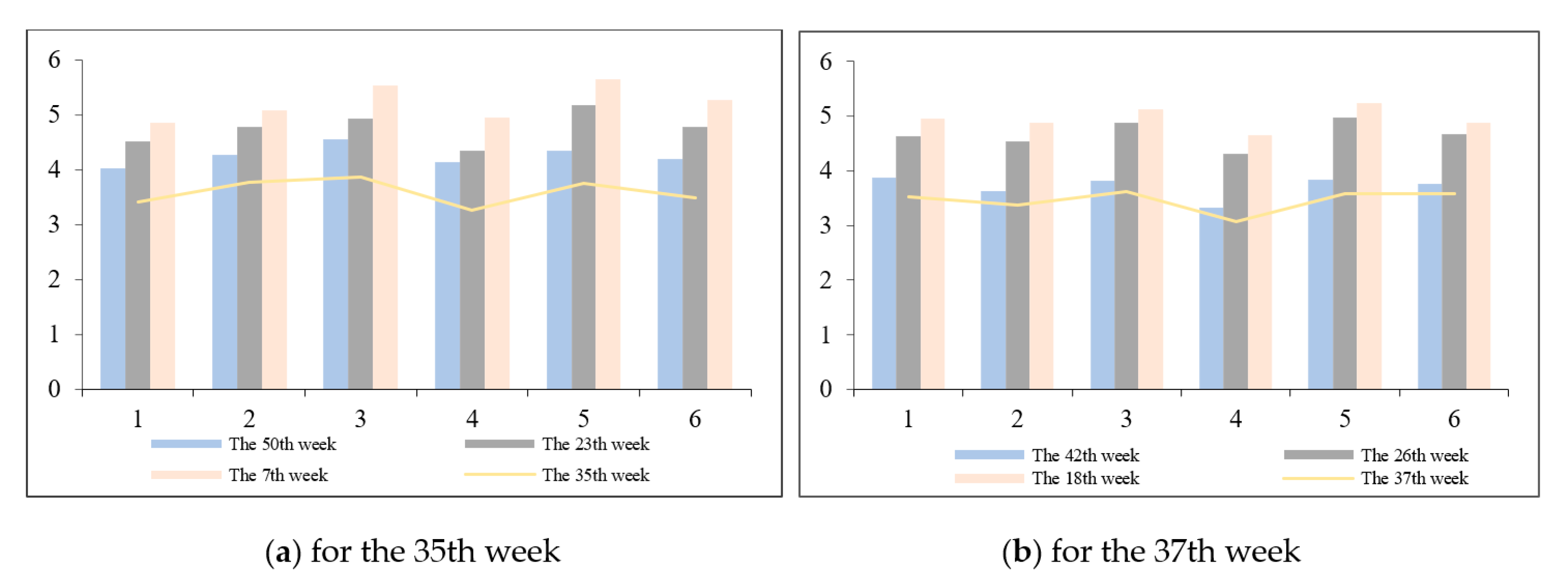
In order to verify the independence and uniform distribution, this paper conducts a correlation graph test (each simulation run 50 times) on the time series of disassembly waste generation. The results show that only 4 of the 52 ${\widehat{\rho }}_k$ values are outside the range of $\pm 1.97/\sqrt{T}$ (α = 0.05), and there is no evidence that the negative null hypothesis is independently distributed. According to the data pattern recognition in DG-HMM, two sets of relatively close data were selected for analysis, and the results are shown in Figure 2. The abscissa in Figure 2 represents the time period (Mon., Tues., Wed., Thur., Fri., and Sat.), and the ordinate represents the amount of disassembly waste. As can be seen from Figure 2a, the data pattern for the 50th week, the 23rd week, and the 7th week is similar to that of the 35th week. Figure 2b shows that the data pattern of the 42nd week, the 26th week, and the 18th week is similar to that of the 37th week.

In this work, the uncertainty of disassembly waste generation was used as a hidden variable. It can be seen from

Table 3. AIC scores of different hidden Markov models.

NHS	NGMC	MLE	AIC	NHS	NGMC	MLE	AIC	NHS	NGMC	MLE	AIC
3	1	388	−168	3	3	325	−63	2	2	397	−185
2	2	306	−49	2	1	359	−102	3	3	364	−124
3	3	385	−153	2	2	312	−58	2	1	372	−135
2	1	328	−68	3	3	355	−94	3	2	393	−174
3	2	341	−73	3	1	369	−127	3	3	377	−146

Note: NHS = the number of hidden states; NGMC = the number of GMM mixture components; MLE = the maximum log-likelihood estimator.

that the value of NHS is two or three, and the value of NGMC ranges from one to three. The minimum and maximum values of MLE are 306 and 397, respectively. The value of AIC ranges from −185 to −49. Regarding AIC standard, the hidden state is set to three, and the mixed component of Gaussian mixture model (GMM) is set to three, as shown in Table 3. Therefore, Uncertainty can be divided into three hidden states, namely, “S”, “M” and “L”. The initial transition probability between different hidden states can be represented by a matrix heat map. The transition matrix (A) is shown in Figure 3, and the color bar represents the transition probability of the matrix (A). The result of the chi-square test shows ${\chi }^2>{\chi }_{\alpha }^2{\left(q-1\right)}^2$, which indicates that the hidden state sequence satisfies the Markov attribute.

4.2.2. Prediction Reliability Analysis

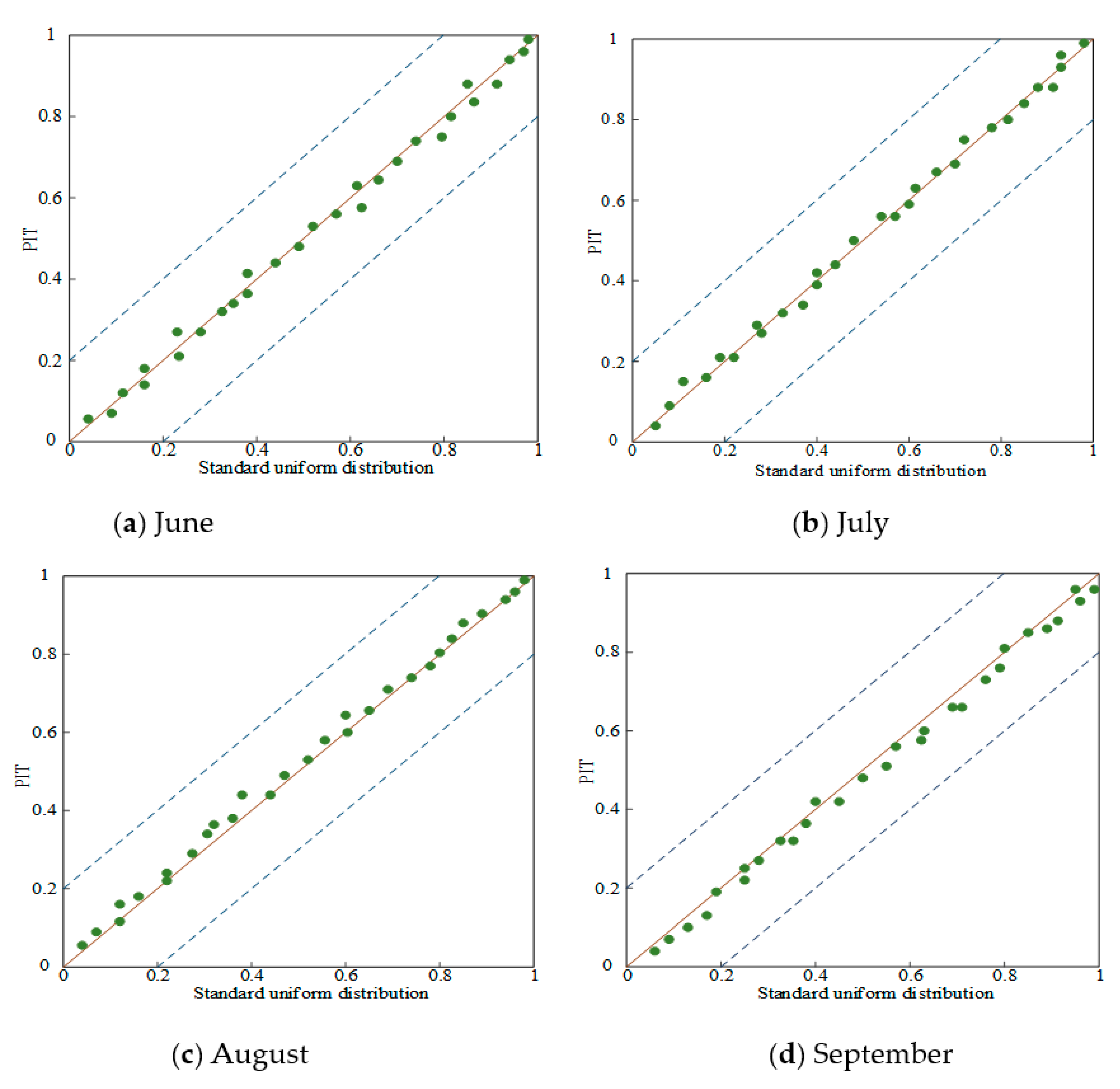
Before determining the rationality of the DG-HMM, its reliability needs to be evaluated. The PIT uniform probability plots illustrate the reliability of the observation values obtained in the monthly forecasting, as shown in Figure 4. It can be seen from Figure 4 that the predicted values of Figure 4c tend to be above the diagonal, and the predicted values of Figure 4d are concentrated below the diagonal. However, the predicted values of Figure 4a,b basically fall on the diagonal. Although the PIT values in August and September deviate slightly from the diagonal, the PIT values are very close to the diagonal. In June and July, the PIT values are within the 5% significant band of Kolmogorov. This shows that the PIT value distribution is quite uniform, and the prediction probability distribution is feasible. There is no prediction of a distribution that is too high or too low. Therefore, it can be explained that the predicted probability distribution is unbiased and with appropriate spread.

4.2.3. Comparison Plots of the Forecast and Observed Value

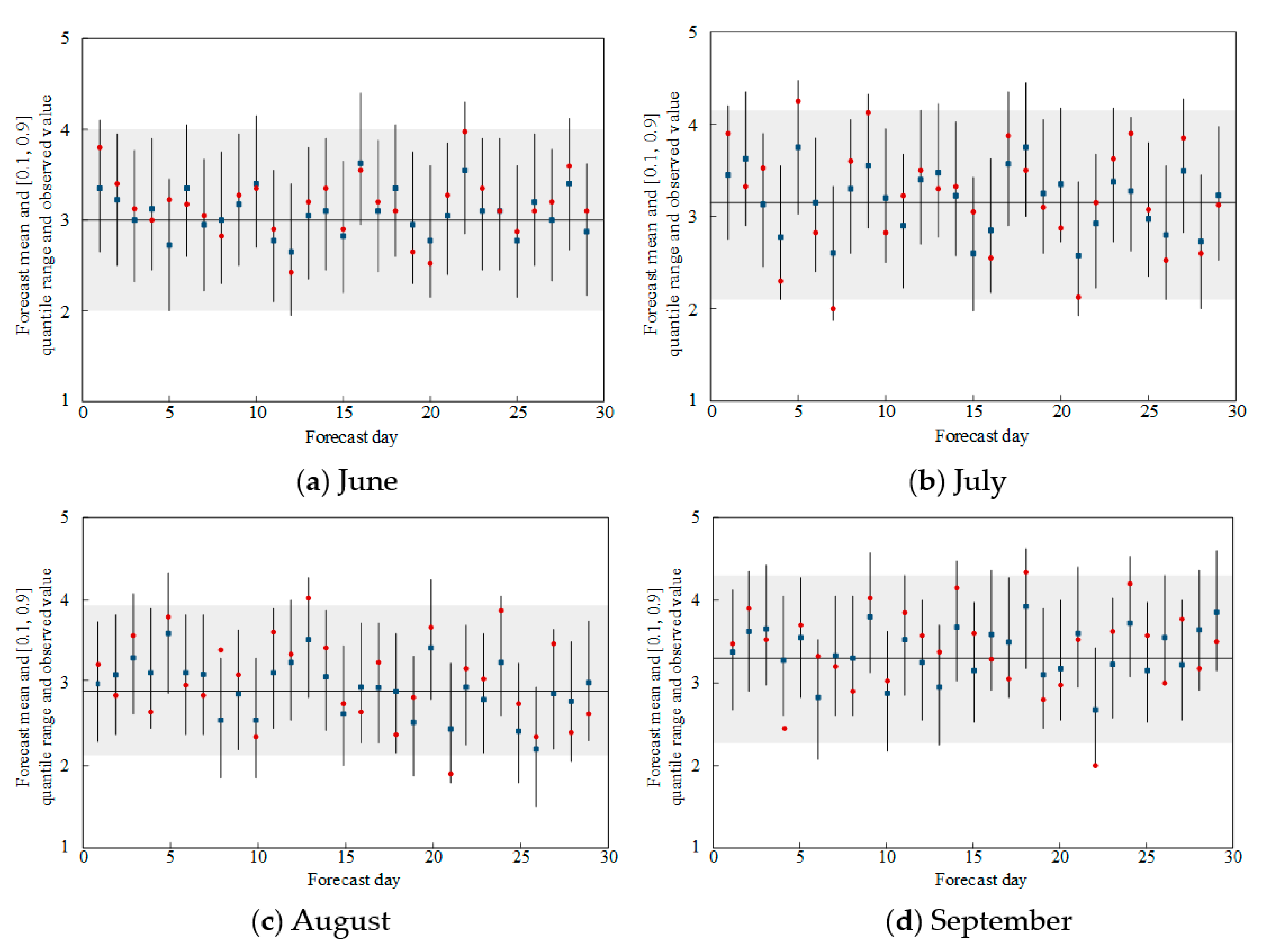
The predicted mean values based on a single observation and the (0.1, 0.9) quantile range are compared in chronological order as shown in Figure 5. The blue square and vertical line are the predicted average and the (0.10, 0.90) quantile range, respectively. The black horizontal line and the shaded area represent the predicted average value and the (0.1, 0.9) quantile range of waste generation, respectively. The red dot represents the observed data. The graph intuitively reflects the comparison between the probability prediction and the actual observation value. As far as the predicted value and the observed value are concerned, the predicted value has no obvious bias trend over time. The black vertical line or the red dot on the shading indicates that the probability prediction or observation value is not biased. It can be seen from Figure 5 that the experimental results of forecast values are very close to the observed values, and few individuals even exceed the observed values. However, the test results of Figure 5a are generally better than those of Figure 5b–d. Regarding the observed values, the fluctuations in the quantile range (0.1, 0.9) in Figure 5b,d are greater than those in Figure 5a,c. For the forecast values, compared with Figure 5a,d, the forecast values in Figure 5b,c fluctuate more greatly in the quantile range (0.1, 0.9). Based on the results of the four-months prediction, the reliability of the DG-HMM is explained.

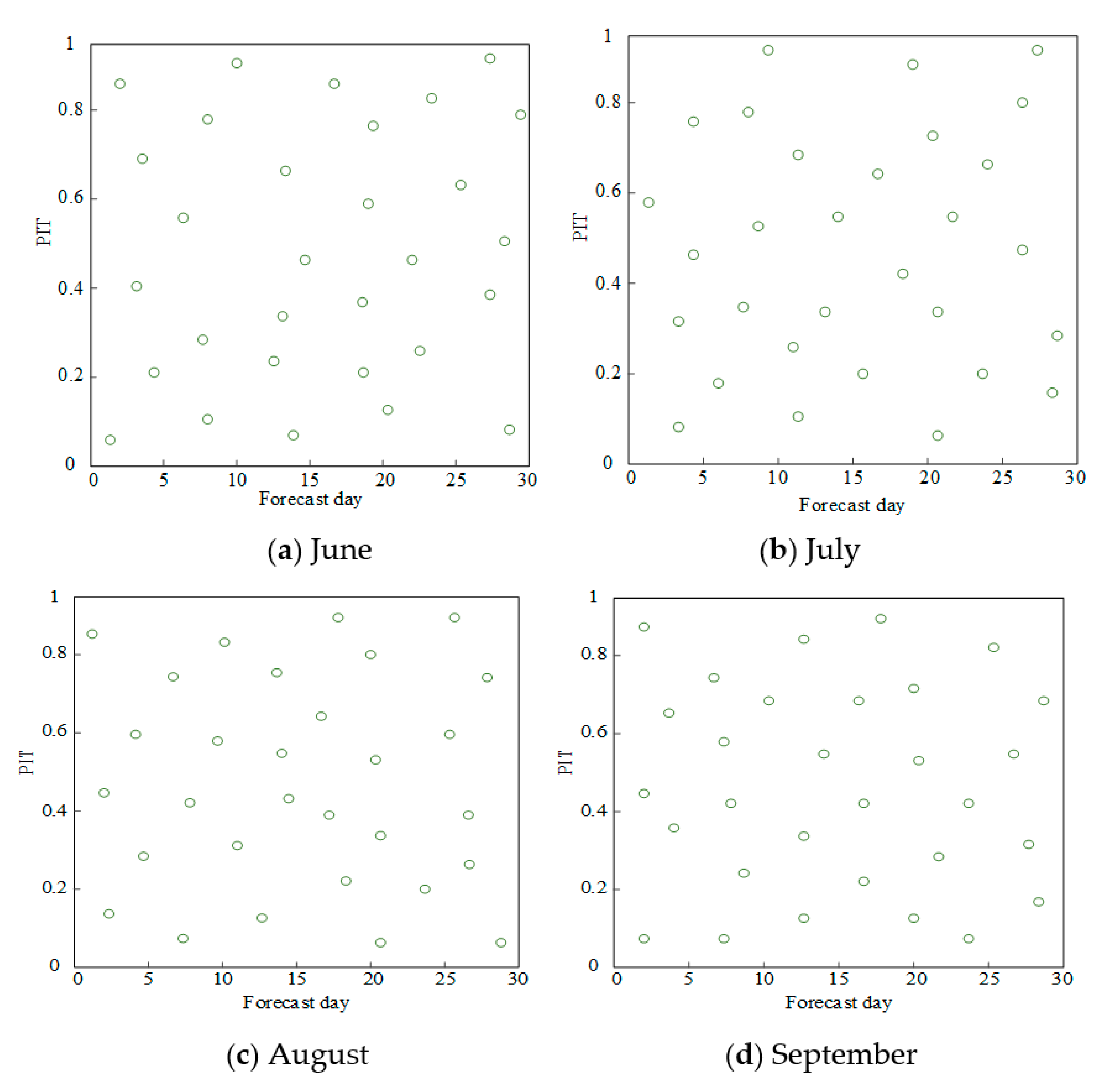
The predicted average values of waste generation are shown in Figure 6 in chronological order. If the prediction is too large, the PIT value is close to one; if the prediction is too small, the PIT value is close to zero. When the prediction unbiased value is 0.50, the effect of prediction distribution is the best. The ideal prediction should produce a uniform distribution of PIT values in (0, 1). As shown in Figure 6a–d, the PIT values are almost evenly distributed, and there is no obvious trend over time or relative to the predicted average.

4.3. Comparative Analysis

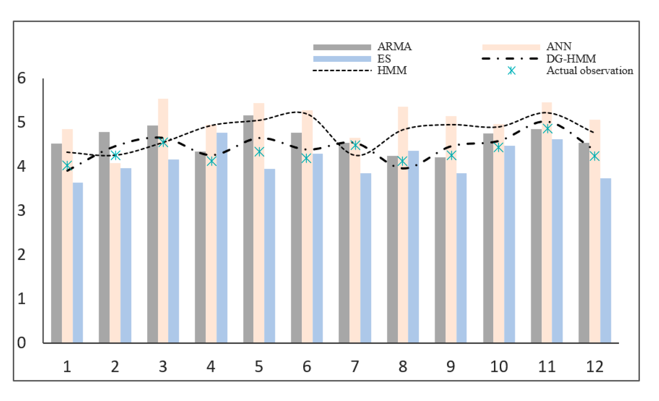
In order to further analyze the performance and comprehensive prediction capabilities of the proposed DG-HMM, the prediction results of ARMA, ES, ANN, HMM and DG-HMM were compared with actual observation data. The average value of prediction in each month was used as the forecast, and the comparison results are shown in Figure 7. As for the overall trend in Figure 7, the prediction average values of EA are undoubtedly lower than the actual observed values, but the predicted values of ANN and HMM are higher than the observed values. Obviously, the predicted values of DG-HMM and ARMA are closer to the observed values. The predicted trends of HMM and DG-HMM are very similar to actual observation, but the values of DG-HMM are closer to the observed values. Although ARMA, ES and ANN have large errors with the observed values, the overall trend is still very close. The MAE, R², and Ȓ² of the prediction results for the five models are shown in

Table 4. Forecasting accuracy of different models for disassembly waste generation.

	ARMA	ES	ANN	HMM	DG-HMM
MAE	18.34	19.60	20.47	16.83	14.35
R2	0.875	0.892	0.899	0.906	0.913
Ȓ2	0.861	0.890	0.874	0.898	0.911

. For MAE, the highest value is ANN (20.47), and the lowest value is DG-HMM (14.35). Regarding R², DG-HMM (0.913) and ARMA (0.875) are the highest value and the lowest value, respectively. For Ȓ², ARMA has a minimum value of 0.861 and DG-HMM shows a maximum value of 0.911. For the variance improvement rate in the models, the maximum improvement rate of ANN is 1.60%, and the minimum improvement rate of DG-HMM is 0.22%, which shows that DG-HMM has the best stability among other models. The MAE, R², and Ȓ² values of DG-HMM are significantly better than the other four models, especially for the criterion of MAE. The analysis results show that DG-HMM performs better predictability than ARMA, ES, ANN and HMM.

5. Conclusions and Discussion

This work proposes a real-time dynamic probability model to predict the amount of disassembly waste generation under uncertainty. We integrate digital twinning, Gaussian mixture, and a hidden Markov model for dynamic prediction of disassembly waste generation. The prediction results show that, in terms of MAE, MSE, R² and Ȓ², the performance of the DG-HMM method is better than that of HMM, ARIMA, ES, ANN and SVM. Based on the MSE skill score, the accuracy of the point prediction obtained by DG-HMM is verified. The unified PIT diagram proves the reliability of DG-HMM. The training results of the example data set show that DG-HMM can effectively solve the problem of predicting disassembly waste generation. Through the model, the prediction will be able to eliminate the uncertainty in disassembly waste generation yield, which allows for more efficient disassembly planning decision making. The DG-HMM model expands the application scope and depth of the traditional input–output method to a certain extent. However, the proposed model is a uniform hidden Markov model, and the waste generation process of the production system is a complex giant system with a huge amount of nonuniform data. Future research on prediction can use virtual simulations and verified methods such as regression analysis, neural networks, or machine learning [45].

With the promotion and application of digital technology, digital management of industrial production and big data simulation will be the future trend [46]. The implementation of clean production and green economy development strategy on technological upgrading will have a significant impact on waste management. Furthermore, the dynamic prediction model established in this study can provide a useful reference for relevant personnel to predict the generation of disassembly waste. Therefore, combining these findings of DG-HMM with real-time disassembly waste generation situations, three policy suggestions are provided on future disassembly management for green remanufacturing. Firstly, enterprises should strengthen the norms and standards for disassembly waste. The forecast trend of the proposed model can provide references for workshop scheduling, process improvement and product life cycle management. Secondly, the government should increase subsidies and policies for disassembly waste disposal. The government’s policy support can promote enterprise to introduce advanced technology and equipment, so as to better improve the management of disassembly waste. Finally, digitizing will be the trend of disassembly waste dynamic prediction and intelligent management in the future. Meanwhile, the real-time data storage of the detection system will provide timely and effective guarantee for disassembly waste prediction.

References

1. Bovea, M.D.; Perez, B.V.; Ibanez, F.V.; Quemades, B.P. Disassembly properties and material characterisation of household small waste electric and electronic equipment. Waste Manag. 2016, 53, 225–236. [Google Scholar] [CrossRef]
2. Jin, T.; Chen, M. Assessing the economics of processing end-of-life vehicles through manual dismantling. Waste Manag. 2016, 12, 384–395. [Google Scholar]
3. Ilgin, M.A.; Gupta, S.M. Environmentally conscious manufacturing and product recovery: A review of the state of the art. J. Environ. Manag. 2010, 91, 563–591. [Google Scholar] [CrossRef]
4. Shao, J.; Huang, S.; Lemus, A.I.; Unal, E. Circular business models generation for automobile remanufacturing industry in China barriers and opportunities. J. Manuf. Technol. Manag. 2020, 31, 542–571. [Google Scholar] [CrossRef]
5. Tian, G.D.; Ren, Y.P.; Feng, Y.X.; Zhou, M.C.; Zhang, H.; Tan, J. Modeling and planning for dual-objective selective disassembly using and or graph and discrete artificial bee colony. IEEE Trans. Ind. Inform. 2019, 15, 2456–2468. [Google Scholar] [CrossRef]
6. Zhang, C.L.; Chen, M. Designing and verifying a disassembly line approach to cope with the upsurge of end-of-life vehicles in China. Waste Manag. 2018, 76, 697–707. [Google Scholar] [CrossRef] [PubMed]
7. Lu, C.; Pan, X.; Chen, X.; Mao, J.; Pang, J.; Xue, B. Modeling of waste flow in industrial symbiosis system at city-region level: A case study of Jinchang, China. Sustainability 2021, 13, 466. [Google Scholar] [CrossRef]
8. Bai, Y.; Ochuodho, T.O.; Yang, J. Impact of land use and climate change on water-related ecosystem services in Kentucky, USA. Ecol. Indic. 2019, 102, 51–64. [Google Scholar] [CrossRef]
9. Grant, S.B.; Saphores, J.D.; Feldman, D.L.; Hamilton, A.J.; Fletcher, T.D.; Cook, P.L.; Marusic, I. Taking the “waste” out of “wastewater” for human water security and ecosystem sustainability. Science 2012, 337, 681–686. [Google Scholar] [CrossRef] [PubMed] [Green Version]
10. Navarro, E.J.; Diamadopoulos, E.; Ginestar, D. Time series analysis and forecasting techniques for municipal solid waste management. Resour. Conserv. Recycl. 2002, 35, 201–214. [Google Scholar] [CrossRef]
11. Chen, H.W.; Chang, N.B. Prediction analysis of solid waste generation based on grey fuzzy dynamic modeling. Resour. Conserv. Recycl. 2000, 29, 1–18. [Google Scholar] [CrossRef]
12. Roubík, H.; Mazancová, J.; Rydval, J.; Kvasnička, R. Uncovering the dynamic complexity of the development of small-scale biogas technology through causal loops. Renew. Energy 2020, 149, 235–243. [Google Scholar] [CrossRef]
13. Setzler, H.; Saydam, C.; Park, S. EMS call volume predictions: A comparative study. Comput. Oper. Res. 2009, 36, 1843–1851. [Google Scholar] [CrossRef]
14. Karpušenkaitė, A.; Ruzgas, T.; Denafas, G. Time-series-based hybrid mathematical modelling method adapted to forecast automotive and medical waste generation: Case study of Lithuania. Waste Manag. Res. 2018, 36, 454–462. [Google Scholar] [CrossRef]
15. Box, G.E.; Tiao, G.C. Intervention analysis with applications to economic and environmental problems. J. Am. Stat. Assoc. 1975, 70, 70–79. [Google Scholar] [CrossRef]
16. Giannouli, M.; Haan, P.; Keller, M.; Samaras, Z. Waste from road transport: Development of a model to predict waste from end-of-life and operation phases of road vehicles in Europe. J. Clean. Prod. 2007, 15, 1169–1182. [Google Scholar] [CrossRef]
17. Chen, Y.; Cai, G.; Zheng, L.; Zhang, Y.; Qi, X.; Ke, S.; Gao, L.; Bai, R.; Liu, G. Modeling waste generation and end-of-life management of wind power development in Guangdong, China until 2050. Resour. Conserv. Recycl. 2021, 169, 105533. [Google Scholar] [CrossRef]
18. Althaf, S.; Babbitt, C.W.; Chen, R. Forecasting electronic waste flows for effective circular economy planning. Resour. Conserv. Recycl. 2019, 151, 104362. [Google Scholar] [CrossRef]
19. Denafas, G.; Ruzgas, T.; Martuzevičius, D.; Shmarin, S.; Hoffmann, M.; Mykhaylenko, V.; Ludwig, C. Seasonal variation of municipal solid waste generation and composition in four east European cities. Resour. Conserv. Recycl. 2014, 89, 22–30. [Google Scholar] [CrossRef]
20. Tian, G.D.; Zhou, M.C.; Li, P. Disassembly sequence planning considering fuzzy component quality and varying operational cost. IEEE Trans. Autom. Sci. Eng. 2017, 81, 1–13. [Google Scholar] [CrossRef]
21. Xiao, F.; Ai, Q. Data-driven multi-hidden Markov model-based power quality disturbance prediction that incorporates weather conditions. IEEE Trans. Power Syst. 2019, 34, 402–412. [Google Scholar] [CrossRef]
22. Peeters, J.R.; Bracqguene, E.; Nelen, D.; Ueberschaar, M.; Van-Acker, K.; Duflou, J.R. Forecasting the recycling potential based on waste analysis: A case study for recycling Nd-Fe-B magnets from hard disk drives. J. Clean. Prod. 2018, 175, 96–108. [Google Scholar] [CrossRef]
23. Karpušenkaitė, A.; Ruzgas, T.; Denafas, G. Forecasting medical waste generation using short and extra short data sets: Case study of Lithuania. Waste Manag. Res. 2016, 34, 378–387. [Google Scholar] [CrossRef] [PubMed]
24. Abdoli, M.A.; Falahnezhad, M.; Behboudian, S. Multivariate econometric approach for solid waste generation modeling: Impact of climate factors. Environ. Eng. Sci. 2011, 28, 627–633. [Google Scholar] [CrossRef]
25. Kannangara, M.; Dua, R.; Ahmadi, L.; Bensebaa, F. Modeling and prediction of regional municipal solid waste generation and diversion in Canada using machine learning approaches. Waste Manag. 2018, 74, 3–15. [Google Scholar] [CrossRef]
26. Intharathirat, R.; Abdul, S.P.; Kumar, S.; Untong, A. Forecasting of municipal solid waste quantity in a developing country using multivariate Grey models. Waste Manag. 2015, 39, 3–14. [Google Scholar] [CrossRef] [PubMed]
27. Chauhan, A.; Singh, A. A hybrid multi-criteria decision making method approach for selecting a sustainable location of health-care waste disposal facility. J. Clean. Prod. 2016, 139, 1001–1010. [Google Scholar] [CrossRef]
28. Noori, R.; Abdoli, M.A.; Farokhnia, A.; Abbasi, M. Results uncertainty of solid waste generation forecasting by hybrid of wavelet transform-ANFIS and wavelet transform-neural network. Expert Syst. Appl. 2009, 36, 9991–9999. [Google Scholar] [CrossRef]
29. Aldieri, L.; Vinci, C.P. Climate change and knowledge spillovers for cleaner production: New insights. J. Clean. Prod. 2020, 271, 122729. [Google Scholar] [CrossRef]
30. Anonymous. Studies from Maejo University yield new data on biofuel (a biorefinery approach for the production of bioethanol from alkaline-pretreated, enzymatically hydrolyzed nicotiana tabacum stalks as feedstock for the bio-based industry). Biotech Week 2021, 20, 996. Available online: link.gale.com/apps/doc/A648765269/AONE?u=nuslib&sid=AONE&xid=1f24d3f7 (accessed on 11 May 2021).
31. Tsai, F.M.; Bui, T.; Tseng, M.; Wu, K. A causal municipal solid waste management model for sustainable cities in Vietnam under uncertainty: A comparison. Resour. Conserv. Recycl. 2020, 154, 104599. [Google Scholar] [CrossRef]
32. Roubík, H.; Mazancová, J.; Phung, L.D.; Banout, J. Current approach to manure management for small-scale Southeast Asian farmers-using Vietnamese biogas and non-biogas farms as an example. Renew. Energy 2018, 115, 362–370. [Google Scholar] [CrossRef]
33. Ahamed, A.; Vallam, P.; Iyer, N.S.; Veksha, A.; Bobacka, J.; Lisak, G. Life cycle assessment of plastic grocery bags and their alternatives in cities with confined waste management structure: A Singapore case study. J. Clean. Prod. 2021, 278, 123956. [Google Scholar] [CrossRef]
34. Bai, R.; Sutanto, M. The practice and challenges of solid waste management in Singapore. Waste Manag. 2002, 22, 557–567. [Google Scholar] [CrossRef]
35. Xiong, C.; Yang, D.; Ma, J.; Chen, X.; Zhang, L. Measuring and enhancing the transfer ability of hidden Markov models for dynamic travel behavioral analysis. Transportation 2018, 47, 585–605. [Google Scholar] [CrossRef]
36. Jiang, P.; Liu, X. Hidden Markov model for municipal waste generation forecasting under uncertainties. Eur. J. Oper. Res. 2016, 250, 639–651. [Google Scholar] [CrossRef]
37. Collin, B.E.; Bruce, E.A.; Susan, M.S. Comparison of Gaussian process modeling software. Eur. J. Oper. Res. 2018, 266, 179–192. [Google Scholar]
38. Sheng, H.M.; Xiao, J.; Wang, P. Lithium iron phosphate battery electric vehicle state-of-charge estimation based on evolutionary Gaussian mixture regression. IEEE Trans. Ind. Electron. 2016, 64, 544–551. [Google Scholar] [CrossRef]
39. Diedrich, A.; Charoensuk, W.; Brychta, R.J.; Ertl, A.C.; Shiavi, R. Analysis of raw microneurographic recordings based on wavelet de-noising technique and classification algorithm: Wavelet analysis in microneurography. IEEE Trans. Biomed. Eng. 2003, 50, 41–50. [Google Scholar] [CrossRef] [PubMed]
40. Bouzida, A.; Touhami, O.; Ibtiouen, R.; Belouchrani, A.; Fadel, M.; Rezzoug, A. Fault diagnosis in industrial induction machines through discrete wavelet transform. IEEE Trans. Ind. Electron. 2011, 58, 4385–4395. [Google Scholar] [CrossRef]
41. Thomas, C.; John, C.; Ramazan, G. Long-run wavelet-based correlation for financial time series. Eur. J. Oper. Res. 2018, 271, 676–696. [Google Scholar]
42. Baum, L.E.; Petrie, T.; Soules, G.; Weiss, N. A maximization technique occurring in the statistical analysis of probabilistic functions of Markov chains. Ann. Math. Stat. 1970, 41, 164–171. [Google Scholar] [CrossRef]
43. Bot, R.I.; Csetnek, E.R.; Vuong, P.T. The forward-backward-forward method from continuous and discrete perspective for pseudo-monotone variational inequalities in Hilbert spaces. Eur. J. Oper. Res. 2020, 287, 49–60. [Google Scholar] [CrossRef]
44. Juan, F.; Rendon, S.; Lilian, M.M. Structural combination of seasonal exponential smoothing forecasts applied to load forecasting. Eur. J. Oper. Res. 2019, 275, 916–924. [Google Scholar]
45. Sakdirat, K.; Lian, Q. Digital twin aided sustainability-based lifecycle management for railway turnout systems. J. Clean. Prod. 2019, 228, 1537–1551. [Google Scholar]
46. Tao, F.; Sui, F.; Liu, A.; Qi, Q.; Zhang, M.; Song, B.; Guo, Z.; Lu, S.C.; Nee, A.Y. Digital twin-driven product design framework. Int. J. Prod. Res. 2018, 57, 3935–3953. [Google Scholar] [CrossRef] [Green Version]
Figure 1. Digital twinning-based architecture of DG-HMM dynamic forecasting.
Sustainability 13 05391 g001
Figure 2. The disassembly waste generation pattern, matched with historical similar data patterns.
Sustainability 13 05391 g002
Figure 3. Matrix plot of transition matrix of supervised DG-HMM using training data.
Sustainability 13 05391 g003
Figure 4. PIT uniform probability plots.
Sustainability 13 05391 g004
Figure 5. Forecasting data and actual observation data plotted chronologically.
Sustainability 13 05391 g005
Figure 6. PIT values plotted chronologically.
Sustainability 13 05391 g006
Figure 7. Forecast and actual observation data.
Sustainability 13 05391 g007