Abstract
The land ecosystem provides essential natural resources for the survival and development of human beings. Therefore, land ecological security (LES) acts as a vital part of the sustainable development of human society and economy. This study included a dynamic analysis of land use change in Chaohu Lake Basin (CLB) in China from 1998 to 2018, evaluating the spatiotemporal patterns of LES at both the administrative district scale and grid scale (200 m× 200 m). Then, geographic detector was applied to analyze the influence of the assessment index on LES. The results show that in the 2008–2018 period, land use changed more significantly compared to the 1998–2008 period. The continuous extension of urban land led to a decrease in the areas of other land use types. In the CLB (administrative district scale), the LES levels varied throughout the study period. In Changfeng, Feixi, and the other three regions, the LES has been significantly improved. However, the LES in six other regions showed different degrees of decline, particularly in Hexian and Urban Hefei. Simultaneously, the LES showed a gradual improvement at a 200 m × 200 m grid scale level. The influence of anthropogenic factors on the LES was stronger than natural factors. Findings from this study provide reliable guidance for improving the ecosystem environment in ecologically fragile areas.
1. Introduction
Ecological security is considered to be a fundamental requirement for economic development and social progress [1]. However, human activities have led to significant changes in the ecological environment. Environmental degradation and pollution emissions have been repeatedly allowed, damaging the region’s natural surface cover, and aggravating industrial pollution and water pollution. Together, these have compromised worldwide ecological security [2,3]. Therefore, more attention has been paid to ecological security issues over time. Ecological security has become a prominent research topic of wide interest [4,5]. The specific concept of ecological security was first proposed by the United States (U.S.) government [6], which articulated that ecological security is a concept with multiple meanings and is part of national and public safety [7,8], with a certain political color [9]. Ecological security can also reflect the integrity and health of the ecosystem, which is defined as the comprehensive status of the human ecosystem [10].
Land ecological security (LES) represents the health of the environment and the sustainability of land resources and ecosystems, steadily providing steady ecological services and filling ecological needs for future generations [11]. Specifically, LES is a complicated system consisting of land natural ecological security, land economic security, and land social security [12]. Since the end of the 1970s, LES has attracted great attention from the government and academia, which has advanced research on the definition of LES and research on environmental safety and change [13]. With the continuous deepening of research on LES, scholarly research has focused on the following aspects: land risk assessment [14], land ecosystem health diagnosis [15,16], ecological service value accounting [17], LES assessment [13], and establishing ecological security patterns [18].
Due to the rapid development of urbanization worldwide, the impacts created by land use change have gradually emerged. Land use transfer has a great impact on regional environment and ecosystem services [19,20]. Human activities can directly affect the LES in a region [21]. Study results have shown that short-term man-made changes in land use can fundamentally change the ecosystem [22,23]. The land use structure has significantly changed with the continuous follow-up of urbanization. With the expansion of urban built-up areas, commercial and industrial demands for land must often be met by adjusting land use patterns (such as cropland land, forestland, water area, and other land-use) [24]. In addition, the constant increase of urban construction land produces pollutants, which seriously harm the ecological environment and which may have an unknown impact on ecological security.
To assess LES, multiple factors including natural, economic, and social factors should be considered [25]. Recently, ecological security assessments have been closely related to ecosystem health assessments, ecological risk assessments, and ecosystem service assessments [5]. The research scale of LES assessment has been continuously expanding, mainly involving cities [5,26], urban agglomerations [27,28], and watersheds [29]. The models have included Driving Force-State-Exposure-Effect-Action (DSEEA) [30], Pressure-State-Response (PSR) [31], and Driving Force-Pressure-State-Impact-Response (DPSIR) [32]. There are many assessment model methods, including the mathematical model method [29], ecological model method [27], and landscape model method [33]. Although there are different framework systems and models to support ecological security assessments, there remains a need for a complete evaluation index system, evaluation standard, and evaluation model [34]. The PSR model is a commonly used model in ecological security assessment. The advantage of this model is that it can deeply reflect the interaction mechanisms between the natural ecosystem and the social ecosystem [35].
Currently, LES assessments are mainly based on the widely-used index system. However, choosing different indices and assessment methods may increase the uncertainty of assessment results [36]. Simultaneously, there remain problems of subjectivity and objectivity in the process of determining the weight [34]; combining subjective and objective methods can avoid the impact of a single method. In addition, as a considerable part of the LES assessment, the security threshold will directly affect the accuracy and scientific nature of the assessment results. However, strong subjectivity in the classification and even a slight adjustment of the threshold may affect the result of LES assessment [37].
Identifying and determining influencing factors are also core issues in ecological security research [36]. Current methods for quantitatively determining the relationship between influencing factors and ecological security include linear regression analysis, generalized additive models (GAM) [13], BP-DEMATEL analysis [36], the geographical detector method, and the improved geographical weighted regression (GWR) model based on the traditional linear regression model. Studies have also combined two of these approaches [38,39]. LES is affected by multiple factors, but most studies have focused on natural factors, such as topography, soil, vegetation coverage, etc. They have not considered the impact of social-economic development and human activities on ecological security, and have not compared the relative importance of different social and ecological factors [40,41]. Therefore, quantifying influencing factors remains a practical problem.
Based on the considerations above, this study analyzed land use change in the Chaohu Lake Basin (CLB) from 1998 to 2018 with respect to changes in quantity and spatial distribution. The study combined the PSR model, analytic hierarchy process, entropy weight method, and comprehensive index model to conduct empirical research on the LES assessment of CLB. First, standardized dimensionless values of all indices were constructed, and the weights of assessment indices were determined, by combining the analytic hierarchy process and entropy weight method. Based on this, the comprehensive index model was used to objectively evaluate the LES, and the geographical detector method was applied to identify the natural and socio-economic factors impacting the spatial change of LES.
2. Data and Methodology
2.1. Study Area
CLB is in the east Chinese Province of Anhui, located between 116°24′–118°0′ E and 29°01′–33°16′ N, and covers an area of 2.04 × 10⁴ km2. The study area consists of 11 administrative districts (Figure 1). The industrial structure is dominated by secondary and tertiary industries. The CLB has been subject to strong human disturbance. It is a key development zone and a vital ecological protection zone in China.
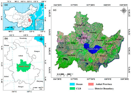
Figure 1.
The study area: (a) the location of Anhui province in China; (b) the location of the Chaohu Lake Basin (CLB) in Anhui province; (c) 11 regions and their geographical locations in the study area and Landsat 8 false color image with the fusion of bands 7, 5, 3 in the study area.
The CLB is one of the five largest freshwater lakes in China. The area has additional rich water resources, with 33 rivers running into Chaohu Lake. The annual average temperature is 15–16 °C and the annual average rainfall is 1100 mm. The overall topography of CLB is high in the west and low in the east, with low-lying plains in the middle, and low mountains and hills all around.
2.2. Data Collection
This study used three categories of data sources: remote sensing (RS) image data, digital elevation model (DEM) data, and socio-economic data. RS images have significant benefits when analyzing land use change. Landsat 5 TM (Thematic Mapper) and Landsat 8 OLI (Operational Land Imager) data were acquired for this study at a resolution of 30 m, for years 2018, 2008, and 1998. All RS image data were downloaded for free from the United States Geological Survey website (USGS, https://earthexplorer.usgs.gov/). The images were selected from the spring season, given the clear features, good vegetation growth, and small cloud cover.
When selecting RS images, it was necessary to integrate two neighbor images to obtain a complete panoramic image of CLB due to its large geographical area. When using two neighbor images, it is ideal if they were acquired on the same date. This is, however, difficult to achieve given image clarity, cloud coverage, and other factors. Nevertheless, land use change in two consecutive years is considered minor, and the image acquisition occurred during the spring, which has a small impact on land use classification. Therefore, this article selected the RS image data presented in Table 1.

Table 1.
Landsat image data used in the study.
Digital elevation model (DEM) data were used to extract terrain information. The ASTER GDEM with a spatial resolution of 30 m was the main data source for DEM data (http://www.giscloud.cn/).
Normalized Difference Vegetation Index (NDVI) reflects the vegetation of regional ecosystem and land use change. NDVI is also a widely applied indicator to quantify ecological status [42] and higher vegetation means safer ecosystems [43]. We used ENVI 5.3 to calculated vegetation cover from RS images, which was shown in Figure 2:
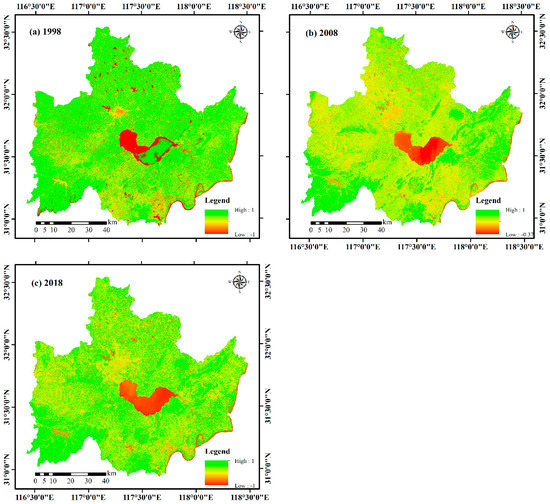
Figure 2.
Map of Normalized Difference Vegetation Index (NDVI) of the CLB in 1998 (a), 2008 (b), and 2018 (c).
The socio-economic data were collected from the Anhui Provincial Social and Economic Statistical Yearbooks. Statistical Yearbooks and socio-economic development Statistics Bulletins for the 11 regions were also used. The data from 1998 to 2018 were selected. All the collected data were converted to raster data at a raster cell of 200 m × 200 m. The details of indices are shown in Table 2:
Table 2.
Data resources for the different indices.
3. Methods
3.1. Land- Use Classification
ENVI 5.3 software was applied to preprocess RS images, including radiometric calibration, atmospheric correction (FLAASH), geometric correction, mosaicing, and subsetting. The Random Forest (RF) model [44] was used to review and classify images based on a random forest classification plug-in named EnMAP-Box. RF, established by Breiman [45], creates multiple decision trees, combined to calculate a classification by randomly replacing the resampled data and altering the predictor sets over the different tree induction developments [46]. The accuracy of the RF classification results depends on the combination of the number of trees and random features two key parameters [47]. To improve the accuracy of the RF model, NDVI [48] and Modified Normalized Difference Water Area Index (MDDWI) [49] two features were applied in the RF model. In addition, we used out-of-bag (OOB) test to estimate the test set accuracy [50], and we set the number of trees and random features at 50 and 3 for classification. According to the China land use/cover remote sensing classification system [51], the land use types were divided into 6 categories: cropland, grassland, forestland, urban land, water area, and other land-use. Figure 3 shows the classification results:
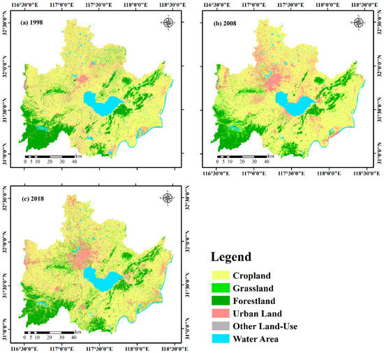
Figure 3.
Land use classification maps of the CLB in 1998 (a), 2008 (b), and 2018 (c).
We verified the classification accuracy of RS images by combining ArcGIS with Google Earth: 500 random points were generated for each phase of the image; these 500 samples were imported into Google Earth to acquire baseline data. The verification results and classification results were imported into Matlab to generate a confusion matrix. The results showed that the overall classification accuracies in 2018 and 2008 reached 88.71% and 88.17%, respectively. The kappa coefficients were 0.8137 and 0.8102, respectively, indicating high classification levels that met application requirements [47]. Due to the lack of high-resolution Google Earth images for 1998, the classification results for that year were not verified. However, based on the same basic conditions of RS images and the same classification method, the classification accuracy was considered to be close to 2008 and 2018.
3.2. Analysis of Land Use Change
3.2.1. Land Use Dynamic Degree Models
Land use dynamic degree expresses the rate of land use change within a certain period [52]. The formula is as follows:
where K represents the land use dynamic degree (%); and represent the area (km2) of a certain land use type at the beginning and the end of a certain period, respectively, and T is the study period (years). K shows whether a single land use type has a negative or positive change, but does not show the contribution of each land category to the overall change.
Land use integrated dynamic degree describes the overall rate of change in land use and degree in a certain period [53]. The equation is as follows:
where (%) stands for the land use integrated dynamic degree; is the area (km2) of the land use type i during the monitoring period; represents the absolute value of the area (km2) of the land use type i converted to j-type land use type during the study period; the units of calculation for the above three parameters are all square km. T is the scope of the study period (years).
3.2.2. Characterizing Land Use Transition
The changing land use trends in the study area are reflected in the dynamic changes in the spatial pattern and quantity of different land use types [54]. The transfer matrix depicts the structural characteristics of the regional land use change and the transfer direction of each land use type. According to the classification results of 1998, 2008, and 2018, the overlay analysis function in ArcGIS was used to generate a utilization transfer matrix for different land use types in 1998–2008, 2008–2018, and 1998–2018, respectively. The mathematical model of the transfer matrix is as follows [55]:
in this formula, represents the area (km2), n represents the number of land types; and i and j represent the land use types at the beginning and end of the study period in the study area, respectively. Each row element of the transfer matrix represents the flowing information of land use, and each column element represents the source information. The transfer matrix shows the land use structure at the beginning and end of the study period, and reflects the transfer of land use types in different periods.
3.3. Assessment of Land Ecological Security
3.3.1. Establishment of the LES Assessment Framework
Multifarious methods have been used for ecological security assessment: the fuzzy evaluation method [34], comprehensive index method [56], landscape ecology [30], and ecological footprint approach [57]. This study constructed a PSR model based on data availability and relevant policy requirements from three aspects: Pressure, State, and Response.
The PSR model was proposed by David [30]; it has been widely used in resource sustainable utilization, ecological security assessment, and environmental assessment [29]. There were two reasons to apply the PSR model for this study. First, the PSR model often provides a clear causal relationship, stressing the interaction between human activities and the ecosystem [58]. When human activities cause a certain degree of pressure (P) on the environment, the state (S) of the environment changes to a certain extent, and people can take certain measures to improve the environment in response (R) to these changes. The actual conditions of CLB and the scientific and dynamic of index selection were used as the starting point of selecting an appropriate index system.
We established a PSR assessment framework, including 16 assessment indices (Table 3) with relevant references. These indices were selected to consider the accessibility and the typicality of data. The pressure subsystem describes the influences of different human activities on the land ecosystem, including population, environment, and economy [59]. The state subsystem depicts the current status or future trends of the land ecosystem. The response subsystem describes a series of measures that people have taken to repair ecosystems and mitigate adverse ecological changes [60].
Table 3.
LES assessment indices of CLB.
3.3.2. Determination of the Assessment Unit
Determining the spatial scope of the assessment unit is a starting point when evaluating and analyzing the regional LES. The size of assessment unit often varies with the amount of data and the size of the assessment area [38]. Most LES assessment studies have applied the administrative unit as the data carrier, because it is a convenient unit for data collection. However, we determined that administrative districts are not suitable for spatial visualization, given the vast expanse of the CLB. Therefore, the administrative district level and grid level were selected as assessment units to ensure the comprehensiveness of the assessment. We adopted the GIS spatial overlay method to determine the grid scale. After several repeated resampling events at different scales and facilitating the calculation, we decided to vectorize and resample the multi-source data to 200 m × 200 m, using the nearest resampling method to reflect the spatial internal differences of the LES in CLB.
3.3.3. Standardization of the Assessment Index
The data sources of an LES assessment reflect different aspects of nature, society, and economy, and different dimensions and distributions of the indices make it difficult to compare them directly [26,38]. This highlighted the need to apply a Range Analysis to normalize the original data. The indices after normalization ranged from 0 to 1. As Table 3 indicates, for a positive trend index, a higher index value was associated with a better LES level. For a negative trend index, a lower index value was associated with a better LES level. The index was standardized as follows [66]:
where represents the standardized value of each index; is the original value of the j-th index of the i-th assessment unit; and and refer to the maximum and minimum values of the j-th index, respectively. Equation (4) calculates the positive index, and Equation (5) calculates the negative index. All aseements indices were exported in the form of raster type data. The paper presents export results for 2018 to conserve space (Figure 4). Export results for 1998 and 2008 are presented in Appendix A.
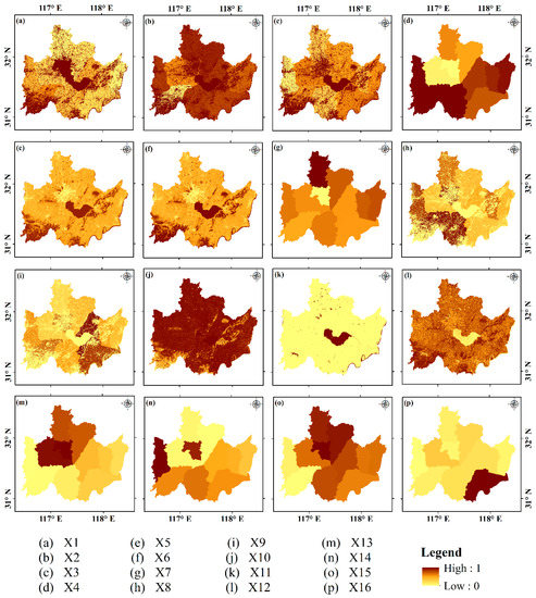
Figure 4.
Raster map of assessment indices for the LES of CLB in 2018 (X1 to X16 represent the 16 assessment indices selected in this study).
3.3.4. Determination of Index Weight
When establishing an ecological security assessment index system, it is critical to determine the weight of each assessment index [67]. This study combined the Analytic Hierarchy Process (AHP) and Entropy weight method to calculate the weight of the ecological security assessment index.
The AHP treats complex problems as a system. The model analyzes the factors in the system and generates an orderly level of interconnection, which combines qualitative and quantitative methods [68,69,70]. The AHP consists of three steps [71]. First, experts judge the relative importance of each index, establishing a relative importance matrix of assessment indices. Second, the eigenvalues of the matrix and the corresponding eigenvectors are calculated [72,73]. Third, the total hierarchy is sorted to determine the weight value of each level factor after the AHP model passes the consistency test.
The entropy weight method is applied to determine the weight of the index according to the value of index information [56]. This makes the calculated weight more realistic, and avoids the subjectivity of calculating different indices under objective conditions [74]. The process is as follows.
According to the definition of entropy, there are n grid units and m assessment indices. As such, the entropy of the assessment index is:
where refers to the entropy value of the i-th index; ; and . We assumed that when , is the value of the j-th index of the i-th assessment unit. Then, Formula (7) was used to generate the entropy weight of the i-th index.
The comprehensive weight was the coefficient of 0.5 for the AHP and the entropy weight method [75]. This was used as the weighted multiplication to generate the comprehensive weight values of the assessment indices for each period (Table 4).
Table 4.
Weights for the assessment index of LES in CLB.
3.3.5. Calculating Comprehensive LES Index
The ecological environment is influenced by natural and economic factors [76]. In this study, the LES comprehensive assessment model was constructed to calculate the index for CLB. The comprehensive ecological security indices of each subsystem were evaluated using the weighted summation method:
where represents the standardized value of the i-th index, and is the weight coefficient value of the i-th index. A greater LES value was associated with a higher ecological security level in the CLB; a lower value was associated with a poorer level of security. Together, these data and formulas can quantitatively reflect the regional ecological security pattern.
3.3.6. Definitions of LES Level
In an ecological security assessment, thresholds are divided using different approaches, including the Equal Interval method, Expert method, and Natural Breaks (Jenks). The key lies in whether the criteria of threshold assessment can distinguish the region’s ecological security status. Traditionally, the LES index has been generally divided into 5 categories according to the Equal Interval method: 0–0.2, 0.2–0.2, 0.4–0.6, 0.6–0.8, and 0.8–1.0 [13,15,26]. The comprehensive index of the LES for the CLB was calculated to determine the range of the index. However, this study found that the calculated ecological security index range using the traditional security level did not effectively reflect the internal differences in the CLB. The Natural Breaks (Jenks) was applied to reclassify the index of LES and the results were adjusted. The results of this revised approach better represented the internal differences of the LES. Consequently, this method was used to delineate the LES thresholds. As a data clustering method [77], the Natural Breaks (Jenks) approach reduces the differences within classes and maximize the differences [78,79]. The LES level [80] definitions for this study are shown in Table 5.
Table 5.
LES levels classification and the definitions of each level.
3.4. Geographical Detector Analysis
The status of LES is the result of multiple factors, and identifying the influencing factors is important for formulating LES protection policies. Therefore, the geographical detector was applied to study the factors influencing the spatial differentiation that impacted the LES, assuming independent variable X and dependent variable Y (comprehensive index of LES). Wang proposed the geographical detector method [81] as a powerful new statistical method to measure “factor forces.” Combined with GIS spatial superposition technology and set theory, this method is applied to detect the spatial heterogeneity of research objects and to quantify how different factors contribute to the results [81].
We assumed the study area consisted of N units, and the LES for each unit was defined as (1 ≤ i ≤ N). The X factor layer was divided into h = 1, …, L stratum. There are Nh units in layer h, and . In layer h, the LES of each unit is defined as Yhi (1 ≤ hi ≤ Nh). For the entire study area, the mean and variance of LES are and , respectively. For layer h, the mean and variance of LES are and , respectively. We used q to measure the explanatory power of each impact factor on the ecological security status, and renamed it as the q-statistic as follows [81]:
where SSW refers to the within sum of the squares; and SST refers to the total sum of squares. Generally, the q value ranges from [0, 1]. The larger the q value is, the more significant the spatial differentiation is, and the stronger the explanatory power of factor X to Y is [82]. The q value was determined using the F test to determine the significance level. For this study, at a 1% significance level, factors with q values greater than 0.2 were selected as the leading influencing factors [83].
4. Results
4.1. Analysis of Land Use Change
4.1.1. Change in the Quantity of Land Use
As shown in Table 6, the land use in the CLB has significantly changed from 1998 to 2018. The significant expansion of urban land led to different degrees of reduction in other land use types. Figure 5 shows that the urban land and the other land-use significantly changed from 1998 to 2008, at a dynamic degree of 1.30% and −4.28%, respectively. The dynamic degree of forestland and water area changes were less than 0, and decreased to a lower extent compared to the other land-use. From 2008 to 2018, the dynamic degree of urban land increased from 1.30% to 1.77%, with quickened growth. The dynamic degree of grassland, cropland, and the other land-use changes showed that a large amount of ecological land was invaded to expand urban land. Moreover, the changes in the other land-use showed a slowing in the pace of decline, compared to from 1998 to 2008. Throughout the study period, cropland, forestland, the other land-use, and the water area all shrank, while the urban land markedly increased.
Table 6.
Characteristic of land use structure in CLB from 1998 to 2018.
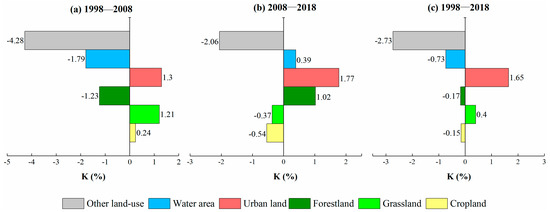
Figure 5.
The land use dynamic degree of each land use type from 1998 to 2018 (a), 2008 to 2018 (b), and 1998 to 2018 (c).
The integrated dynamic degree of land use provides an overall impression of the intensity of land use types from 1998 to 2018 (Table 7). The land use integrated dynamic degree in the CLB was 1.31% from 1998 to 2008, and was 1.42% from 2008 to 2018, showing an upward trend. This also indicated that land use changed more strongly compared with 1998–2008.
Table 7.
Land use integrated dynamic degree (LC) in CLB from 1998 to 2018.
4.1.2. Characterizing the Transfer Direction of Land Use
We established a land use transfer matrix from 1998 to 2018 using the Tabulate Area tool of ArcGIS. The results are shown in Table 8 and Figure 6:
Table 8.
Transfer matrix of land use types in CLB from 1998 to 2018 (km2).
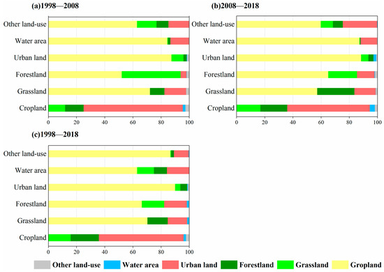
Figure 6.
Transfer rate of land use types in CLB from 1998 to 2008 (a), 2008 to 2018 (b), and 1998 to 2018 (c).
Land use transfers in the CLB from 1998 to 2018 showed the following characteristics according to Table 8 and Figure 6. (1) Conversion to cropland was the main land use transfer characteristic. The transfer rates of grassland, urban land, forestland, and the other land-use type, as well as water area, reached 70.41%, 90.01%, 66.37%, 86.66%, and 63.03%, respectively. The transformed areas of urban land reached 1222.81 km2. The transfer rates of forestland, urban land, and water area from 2008 to 2018 improved compared to 1998 to 2008, while the transfer rates of grassland and the other land-use type showed a downward trend. (2) The cropland was principally transformed into urban land; the transformed areas accounted for 70.41%, 58.51% and 60.15% in 1998–2008, 2008–2018, and 1998–2018, respectively. The conversion from cropland to grassland and forestland was relatively high, accounting for approximately 40% of the total cropland transfer rate.
4.1.3. Land Use Change Spatial Map Analysis
In this study, the thematic change workflow in ENVI 5.3 was used to generate land use spatial transfer map based on the land use data from 1998 to 2018 in the CLB. Through this process, the spatial distribution characteristics of the land use type conversions were revealed and analyzed, which is showed in Figure 7.
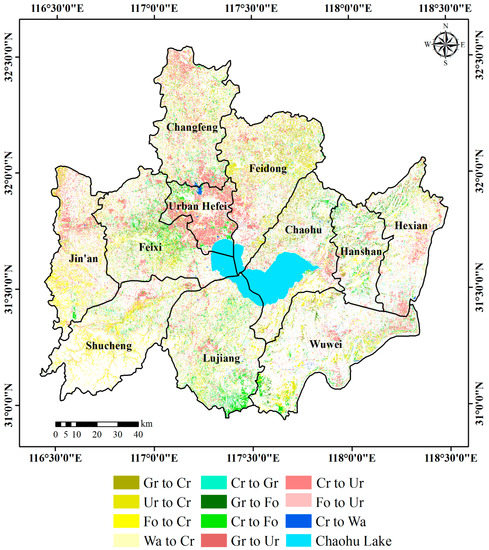
Figure 7.
Transfer map of land use from 1998 to 2018 in CLB (the abbreviations Gr, Cr, Ur, Fo and Wa in the legend represent grassland, cropland, forestland, water area, and the other land-use type, respectively).
The main spatial characteristics of land use type conversions in CLB from 1998 to 2018 (Figure 7) were as follows. The urban land was mainly converted from cropland, grassland, and forestland. This occurred in Fexi, Urban Hefei, Changfeng, Feidong, and Hexian; and demonstrates the spreading characteristics from Urban Hefei to the surrounding areas. The phenomenon of cropland expansion was the most significant trend, and was distributed in the whole region. Forestland was intensively converted to cropland in Jin′an, Shucheng, and Lujiang, which lie among high-altitude and high-slope mountains. The increase of forestland occurred in Lujiang, Feixi, and Wuwei.
4.2. Land Ecological Security Assessment
4.2.1. Overall Characteristics of LES in Municipal Areas
This study used administrative districts as the assessment unit to reflect the ecological security status of the CLB at a macro scale. Using Formula (7) and the collected statistical data, RS data, land use data, and DEM data of administrative districts, we calculated the county LES. The results are shown in Figure 8.
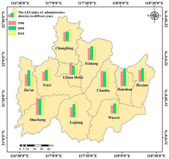
Figure 8.
The LES index of administrative districts in CLB from 1998 to 2018.
In 1998, there was no significant difference in the LES value at the administrative district scale in the CLB. The LES levels were higher in Shucheng and Chaohu compared to other regions. In 2008, the LES levels of most counties had increased to varying degrees; nevertheless, the LES levels in Hexian and Urban Hefei showed a downward trend. For example, the LES in Urban Hefei decreased from 0.4174 to 0.3333. In 2018, the LES levels in most regions showed different trends compared to 2008. In Hexian, Hanshan, Jin’an, and Feidong, there was a decreasing trend; the other seven regions showed an increasing trend. The highest comprehensive index value was in Chaohu (0.6216), followed by Shucheng; Urban Hefei had the lowest value.
4.2.2. Characteristics of Spatial Structure of LES Based on Grid
To further understand the spatial differences of LES in the administrative districts of CLB, ArcGIS 10.2 was used to describe the spatial situation. Furthermore, we calculated the number of grid units at each level, as shown in Table 9 and Figure 9.
Table 9.
Proportion of LES levels of CLB from 1998 to 2018.
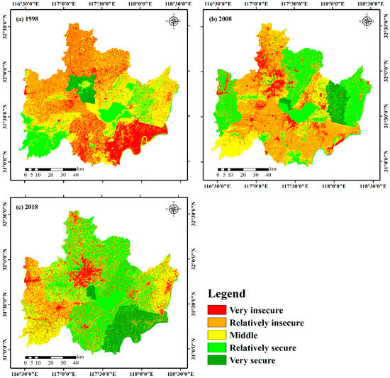
Figure 9.
Spatial patterns of LES in CLB in 1998 (a), 2008 (b), and 2018 (c).
The LES in the CLB showed a positive trend from 1998 to 2018. In 1998, approximately 35.93% of the CLB was at the “very insecure” level; approximately 27.80% was at the “middle” level; and only 2.96% of the study area was at the “very secure” level. In 2008, the “very insecure” level decreased to 9.22% from 19.05%. The “relatively secure” area expanded from 14.26% to 27.54%. The areas designated as the “middle” level and above significantly increased from 45.02% to 54.05%. The “middle” areas increased to 28.62% in 2018 and the “very secure” areas expanded significantly. The “relatively secure” level accounted for 33.08% of the study area, which was a significant change from 2008.
In terms of spatial structure, 19.05% of CLB was at the “very insecure” level in 1998, with a small spatial difference between the northern and southern regions. The horizontal distribution of LES was lower in the west compared to the east. In 2008, the LES of the western and eastern regions significantly changed; the LES of the southern regions also improved. The areas of the “relatively secure” level continued to expand, and the areas at the “relatively secure” level exhibited a spatial evolution from decentralization to aggregation. Compared with 2008, the LES of the eastern and western CLB decreased in 2018, while the LES of the northern and southern regions continued to rise. The advantage of the “very secure” level gradually emerged. Generally speaking, the LES in CLB significantly changed in the northern and southern regions from 1998 to 2018, with a significant broadening of the ecological security level. The change in the LES pattern was relatively slow in the southwest region. This is because the Dabie Mountains were less disturbed by human activities and had higher vegetation coverage; as such, the LES was relatively high and did not significantly change.
4.3. Identification of Influencing Factors of LES
This study classified the input data and applied the Natural Breaks method in ArcGIS to convert the influencing factors from continuous variables to discrete variables. The fishnet tool was adopted to extract raster data to the point. The sampling interval was set at 3 km to generate 2437 uniform distribution points covering different land use types and LES levels in the CLB. Then, we extracted the attributes of each index using the Extract Multi Values to Point tool in ArcGIS 10.2. The power of determinant values (q) was calculated using the geographical detector method (Figure 10).
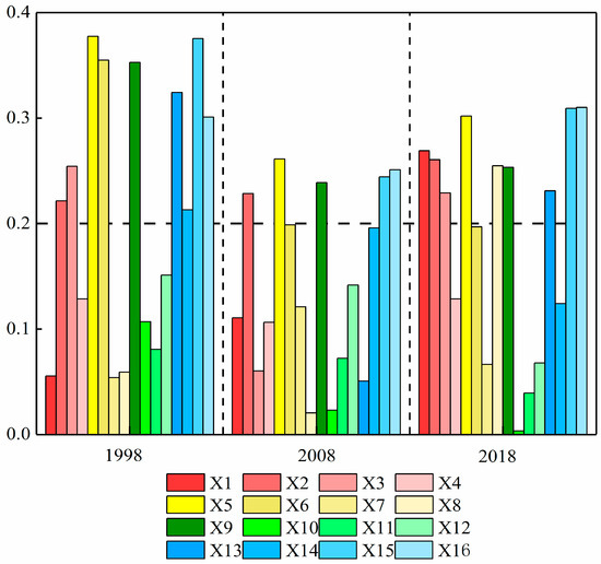
Figure 10.
The detection results of geographical detector factors from 1998 to 2018 (X1 to X16 represent the 16 assessment indices selected in this study).
In 1998, the influence of the explanatory power on the LES of each index factor in the CLB was ranked as follows: the highest q value was for X5 (0.3775), followed by X15 (0.3754), X6 (0.3549), X9 (0.3528), X13 (0.3244), X16 (0.3010), X3 (0.2543), and X2 (0.2217). In 2008, the q value of X5 ranged from 0.3775 to 0.2613, indicating a more powerful effect compared to other indices. The influences of the X5, X6, and X9 on LES gradually weakened from 1998 to 2008. The factors X2, X15, and X16 had significant impacts on LES with q values of 0.2285, 0.2443 and 0.2510, respectively. In 2018, the X16 factor had the strongest influence on LES, with a q value of 0.3101; X15 was a close second, with a q value of 0.3093. Factors X1 and X5 also had strong influences on LES. Meanwhile, the q value of X1 reached its highest values during the study period.
5. Discussion
5.1. Driving Forces of Land Use Change in CLB
Breaking from the traditional assessment of watershed ecological security, this study first analyzed the impact of land use change on the regional ecological environment, providing support for studying the impact of human activities on the LES [64]. From 1998 to 2018, significant changes have occurred to the land use in the CLB: the urban land in the built-up areas increased significantly during the study period; and areas of cropland, forestland, and water area were continuously occupied. A previous study of Zhoushan also found that urban areas had invaded a large amount of productive land, with results that were similar to this study [63]. Although both the transition of the natural environmental and social-economic activities drove changes in land use [1], social-economic activities had a greater impact in a short term. The land use integrated dynamic degree was essentially consistent with the dynamic changes in urban land. This illustrated that the urbanization and expansion of built-up areas were principal forces driving land use in CLB.
Since the reform and opening up, CLB counties have invested significant effort to develop the economy and accelerate urbanization by relying on their resource advantages. This has greatly improved people’s living standards. However, the conflicts between economic development, population, resources, and the ecological environment have become increasingly prominent [84], and the area of ecological scale land has been continuously reduced. Meanwhile, due to the increasing anthropogenic activities in the CLB, the lake has suffered from critical pollution and eutrophication [85].
5.2. Analysis of the LES Pattern in CLB
Concrete assessment units must be established before conducting an LES assessment. This study selected the administrative district scale and a grid scale of 200 m × 200 m to conduct the LES assessment. The administrative district scale facilitates the determination of ecological protection and construction achievements, and facilitates a horizontal comparison with other internal regions. Compared with the LES assessment at a large grid scale, a smaller scale [13,86] was able to better reflect the spatial differences of regional LES changes [38]. In addition, the entropy weight method and the AHP were combined to determine the weight, instead of using objective or subjective methods to determine the weight alone [87,88].
At the administrative district scale, Chaohu and Shucheng experienced an improvement of the ecological environment from 1998 to 2018, with a consistently high LES level due to the high vegetation coverage and abundant rivers in these regions. This finding was consistent with the study of Hu et al. [76]. The level of ecological security of Urban Hefei changed significantly; while the urbanization level in some areas increased, there was an insufficient emphasis on the natural environment. Therefore, more attention needs to be paid to ecologically restoring these counties to improve the ecosystem level.
We estimated the spatial differentiation of LES within the CLB. From 1998–2008, expanded areas of the CLB became “relatively insecure” instead of the dominant “very insecure” designation in 1998. This expansion extended across the northern and southern areas of the CLB, particularly in the southern areas, where the area denoted “relatively insecure” had grown substantially. From 2008 to 2018, the areas denoted as “middle” and “above” levels in the CLB continuously expanded, changing from “relatively insecure” to “middle” in grid units in Chaohu, Lujiang, Wuwei, and Changfeng. Despite the increasing level of urbanization, more attention and investment were placed in ecological protection [28]. The government gradually began to balance urbanization and environmental protection, strengthening the implementation of ecological protection measures. Meanwhile, rapid urbanization in China led to the continuous expansion of urban land, which promoted the degradation of LES to different degrees [12]. In this study, the variations in LES were similar to the expansion of urban land; this result was consistent with the study of Li et al. (2020) [28]. The CLB was the main urbanization area in Anhui Province from 2003 to 2013 [89]. As urbanization accelerated, the built-up area expanded; however, the expansion of urban areas into suburban areas are expected to affect regional ecological security [28]. The regions with high LES were stably distributed in areas with fewer human activities and abundant vegetation, lakes, and other abundant water resources. This was consistent with the general research results [5,28,90].
5.3. Analysis of Influencing Factors of LES
The relationship between LES and its influencing factors is complex [13]. In this study, human factors had a stronger impact on the LES in the CLB than natural factors. These human factors included the electricity consumption per cropland area, pesticide use per cropland area, land use intensity, anthropogenic disturbance index, per capita net income of farmers, and afforestation area.
The anthropogenic disturbance index has been shown to have an essential influence on the regional LES [59]. Similarly, the anthropogenic disturbance index performed significantly in this study, indicating the impact of human activities on the ecosystem. Land use and land cover change (LULCC) can be measured through land use intensity, which has also been shown to influence the ecosystem [61,91]. Recently, the land use pattern in CLB has experienced the conversion of cropland to industrial land [85], producing significant environmental waste. Pesticide and fertilizer pollution in the ecological environment has been manifested in the pollution of soil, water, and air. Studies have also shown that environmental pollution is an important factor affecting the regional LES [92,93,94]. A similar study showed that the index of environment pollution treatment investment, a positive influencing factor, was concentrated in regions with poor ecological conditions in the study area. A higher factor index was associated with improvements to the ecological environment [59]. The factor of the pesticides per cropland area also strongly influenced the LES of the CLB. As agricultural modernization has continued, agricultural development has increased in scale and industrialization. As the main land use type in CLB, cropland has been associated with environmental pollution caused by pesticide and fertilizer use, which does not support the stability of the regional LES.
The CLB has experienced rapid development, with changes to its resources and economy. Simultaneously, the increase in the effective area of cropland will consume more electricity through agricultural irrigation [95]. Therefore, this factor influenced the LES, explaining the high spatial variability in LES from 1998 to 2018. The q values of the factor afforestation area indicated an intense effect on LES. Urban green infrastructure is considered to be the “natural life support system” of a city [96]. The afforestation areas of the whole Anhui Province have reached 1.43 × 10⁶ acres, because the government has steadily advanced actions to promote greenness and efficiency, and human activities have led to large-scale afforestation. The factor of the per capita net income of farmers describes the living standards of farmers and population distribution in the study area [59]. The results of the geographical detector method indicated that this factor had a prominent impact on the LES.
The impact of natural factors on the LES in CLB was not significant. The impact of soil erosion factors and the distance between residential areas on ecological security, selected by Liu et al. [38] using the OLS-GWR model, showed significant spatio-temporal heterogeneity. Moreover, the soil erosion factor had the most significantly negative impact on ecological security. However, this factor was not considered in this study’s assessment index system. Furthermore, the NDVI of natural factors did not strongly influence the LES, which is consistent with previous studies [36,59].
5.4. Limitations
Like all studies, this one had some limitations. First, we were unable to collect sufficient data at a small scale, because some of the data were only available at the scale of the administrative district. For example, indices related to pesticide and fertilizer use are only available at the administrative district level. This resulted in a low spatial position accuracy. To facilitate calculations, the assessment scale used for the study was based on a 200 m × 200 m grid unit. In the future, resampling could be considered to conduct the research at a finer level of precision [59]. Secondly, the relationship between natural factors and land use is seldom considered in the analysis of land use change, which can be further discussed in future. Finally, although the geographical detector can measure the explanatory power of factors, it cannot explain whether the influence is positive or negative. Future studies should further identify this information.
6. Conclusions
This study generated land use information from 1998 to 2018 using RF classification and analyzed the land use change in the CLB. After that, we mapped the land use spatial patterns at an administrative district scale and grid scale. Further, the contribution of the index factors to the distribution of the LES pattern were assessed, using the geographic detector method. From our results, we conclude that:
- The significant expansion of urban land led to different degrees of reduction in other land use types. In addition, more significant land use change occurred from 2008 to 2018 compared to 1998–2008 in the CLB. The cropland was the main converted direction of other land use types and urban land was mainly converted from cropland, grassland, and forestland.
- In the CLB (administrative district scale), the LES levels varied throughout the study period. The LES improved significantly in five regions, namely Changfeng, Lujiang, Wuwei, Chaohu and Feixi. However, the LES in other six regions showed different degrees of decline, especially in Hexian and Urban Hefei. At the grid scale, the LES in CLB showed a gradual improvement trend.
- Anthropogenic factors, such as electricity consumption per cropland area, pesticide use per cropland area and anthropogenic disturbance index had stronger impacts on LES than natural factors (e.g., NDVI).
The research results of this paper contribute to future quantitative analyses of the LES pattern of the CLB. At the same time, we quantified the impact of each assessment index factor on LES, providing insights for local governments to optimize urban planning and improve the ecological environment.
Author Contributions
Conceptualization, M.W., T.Z., L.L. and L.C.; methodology, M.W.; validation, M.W. and J.W.; software, W.L.; formal analysis, M.W.; data curation, T.Z., Y.Z. and L.Y.; writing-original draft preparation, M.W., J.W. and W.L.; writing-review and editing, T.Z., L.L., L.C. and S.H.; visualization, J.W., W.L.; supervision, project administration, and funding acquisition, L.C. All authors have read and agreed to the published version of the manuscript.
Funding
The research was funded by the Fundamental Research Funds for the Central Universities under grant number 2018ZDPY07.
Institutional Review Board Statement
Not applicable for this study.
Informed Consent Statement
Not applicable for this study.
Data Availability Statement
The input data in this research can be accessed freely from online sources.
Acknowledgments
The authors thank the United States Geological Survey (USGS) for freely providing the satellite RS image data used in this study. Furthermore, we appreciate the editors and reviewers for their constructive comments and suggestions.
Conflicts of Interest
The authors declare no conflict of interest.
Appendix A

Figure A1.
Raster map of assessment indices for the LES of CLB in 1998. X1 to X16 represent the 16 assessment indices selected in this study.
Figure A1.
Raster map of assessment indices for the LES of CLB in 1998. X1 to X16 represent the 16 assessment indices selected in this study.


Figure A2.
Raster map of assessment indices for the LES of CLB in 2008. X1 to X16 represent the 16 assessment indices selected in this study.
Figure A2.
Raster map of assessment indices for the LES of CLB in 2008. X1 to X16 represent the 16 assessment indices selected in this study.

References
- Chai, J.; Wang, Z.; Zhang, H. Integrated evaluation of coupling coordination for land use change and ecological security: A case study in Wuhan city of Hubei province, China. Int. J. Environ. Res. Public Health 2017, 14, 1435. [Google Scholar] [CrossRef] [PubMed]
- Vörösmarty, C.J.; McIntyre, P.B.; Gessner, M.O.; Dudgeon, D.; Prusevich, A.; Green, P.; Glidden, S.; Bunn, S.E.; Sullivan, C.A.; Liermann, C.R.; et al. Global threats to human water security and river biodiversity. Nature 2010, 467, 555–561. [Google Scholar] [CrossRef] [PubMed]
- Čuček, L.; Klemeš, J.J.; Varbanov, P.S.; Kravanja, Z. Significance of environmental footprints for evaluating sustainability and security of development. Clean Technol. Environ. Policy 2015, 17, 2125–2141. [Google Scholar] [CrossRef]
- Chen, H.S. Evaluation and Analysis of Eco-Security in Environmentally Sensitive Areas Using an Emergy Ecological Footprint. Int. J. Environ. Res. Public Health 2017, 14, 136. [Google Scholar] [CrossRef] [PubMed]
- Zhao, C.R.; Zhou, B.; Su, X. Evaluation of urban eco-security-A case study of Mianyang City, China. Sustainability 2014, 6, 2281–2299. [Google Scholar] [CrossRef]
- Ezeonu, I.C.; Ezeonu, F.C. The environment and global security. Environmentalist 2000, 20, 41–48. [Google Scholar] [CrossRef]
- Huang, Q.; Wang, R.; Ren, Z.; Li, J.; Zhang, H. Regional ecological security assessment based on long periods of ecological footprint analysis. Resour. Conserv. Recycl. 2007, 51, 24–41. [Google Scholar] [CrossRef]
- Geneletti, D.; Beinat, E.; Chung, C.J.F.; Fabbri, A.G.; Scholten, H.J. Accounting for uncertainty factors in biodiversity impact assessment: Lessons from a case study. Environ. Impact Assess. Rev. 2003, 23, 471–487. [Google Scholar] [CrossRef]
- Spring, U.O. The future of humanity: Human, gender and ecological security. Peace Confl. J. Peace Psychol. 2000, 6, 229–235. [Google Scholar] [CrossRef]
- Yu, G.; Zhang, S.; Yu, Q.; Fan, Y.; Zeng, Q.; Wu, L.; Zhou, R.R.; Nan, N.; Zhao, P. Assessing ecological security at the watershed scale based on RS/GIS: A case study from the Hanjiang River Basin. Stoch. Environ. Res. Risk Assess. 2014, 28, 307–318. [Google Scholar] [CrossRef]
- Feng, Y. Modeling dynamic urban land-use change with geographical cellular automata and generalized pattern search-optimized rules. Int. J. Geogr. Inf. Sci. 2017, 31, 1198–1219. [Google Scholar] [CrossRef]
- Xu, L.; Yin, H.; Li, Z.; Li, S. Land Ecological Security Evaluation of Guangzhou, China. Int. J. Environ. Res. Public Health 2014, 11, 10537–10558. [Google Scholar] [CrossRef] [PubMed]
- Feng, Y.; Yang, Q.; Tong, X.; Chen, L. Evaluating land ecological security and examining its relationships with driving factors using GIS and generalized additive model. Sci. Total Environ. 2018, 633, 1469–1479. [Google Scholar] [CrossRef] [PubMed]
- Travis, C.C.; Morris, J.M. The Emergence of Ecological Risk Assessment1. Risk Anal. 1992, 12, 167–168. [Google Scholar] [CrossRef]
- Sun, B.; Tang, J.; Yu, D.; Song, Z.; Wang, P. Ecosystem health assessment: A PSR analysis combining AHP and FCE methods for Jiaozhou Bay, China1. Ocean Coast. Manag. 2019, 168, 41–50. [Google Scholar] [CrossRef]
- Shepherd, K.D.; Shepherd, G.; Walsh, M.G. Land health surveillance and response: A framework for evidence-informed land management. Agric. Syst. 2015, 132, 93–106. [Google Scholar] [CrossRef]
- Sutton, P.C.; Anderson, S.J.; Costanza, R.; Kubiszewski, I. The ecological economics of land degradation: Impacts on ecosystem service values. Ecol. Econ. 2016, 129, 182–192. [Google Scholar] [CrossRef]
- Wang, Y.; Pan, J. Building ecological security patterns based on ecosystem services value reconstruction in an arid inland basin: A case study in Ganzhou District, NW China. J. Clean. Prod. 2019, 241, 118337. [Google Scholar] [CrossRef]
- Nuissl, H.; Haase, D.; Lanzendorf, M.; Wittmer, H. Environmental impact assessment of urban land use transitions-A context-sensitive approach. Land Use Policy 2009, 26, 414–424. [Google Scholar] [CrossRef]
- Ojoyi, M.M.; Mutanga, O.; Odindi, J.; Kahinda, J.M.M.; Abdel-Rahman, E.M. Implications of land use transitions on soil nitrogen in dynamic landscapes in Tanzania. Land Use Policy 2017, 64, 95–100. [Google Scholar] [CrossRef]
- Liu, Y.; Hou, X.; Li, X.; Song, B.; Wang, C. Assessing and predicting changes in ecosystem service values based on land use/cover change in the Bohai Rim coastal zone. Ecol. Indic. 2020, 111, 106004. [Google Scholar] [CrossRef]
- Juanita, A.D.; Ignacio, P.; Jorgelina, G.A.; Cecilia, A.S.; Carlos, M.; Francisco, N. Assessing the effects of past and future land cover changes in ecosystem services, disservices and biodiversity: A case study in Barranquilla Metropolitan Area (BMA), Colombia. Ecosyst. Serv. 2019, 37, 100915. [Google Scholar] [CrossRef]
- Wu, Y.; Tao, Y.; Yang, G.; Ou, W.; Pueppke, S.; Sun, X.; Chen, G.; Tao, Q. Impact of land use change on multiple ecosystem services in the rapidly urbanizing Kunshan City of China: Past trajectories and future projections. Land Use Policy 2019, 85, 419–427. [Google Scholar] [CrossRef]
- Xu, C.; Pu, L.; Zhu, M.; Li, J.; Chen, X.; Wang, X.; Xie, X. Ecological security and ecosystem services in response to land use change in the coastal area of Jiangsu, China. Sustainability 2016, 8, 816. [Google Scholar] [CrossRef]
- Su, S.; Chen, X.; DeGloria, S.D.; Wu, J. Integrative fuzzy set pair model for land ecological security assessment: A case study of Xiaolangdi Reservoir Region, China. Stoch. Environ. Res. Risk Assess. 2010, 24, 639–647. [Google Scholar] [CrossRef]
- Su, S.; Li, D.; Yu, X.; Zhang, Z.; Zhang, Q.; Xiao, R.; Zhi, J.; Wu, J. Assessing land ecological security in Shanghai (China) based on catastrophe theory. Stoch. Environ. Res. Risk Assess. 2011, 25, 737–746. [Google Scholar] [CrossRef]
- Yang, Y.; Cai, Z. Ecological security assessment of the Guanzhong Plain urban agglomeration based on an adapted ecological footprint model. J. Clean. Prod. 2020, 260, 120973. [Google Scholar] [CrossRef]
- Li, Z.T.; Li, M.; Xia, B.C. Spatio-temporal dynamics of ecological security pattern of the Pearl River Delta urban agglomeration based on LUCC simulation. Ecol. Indic. 2020, 114, 106319. [Google Scholar] [CrossRef]
- Shen, Y.; Cao, H.; Tang, M.; Deng, H. The human threat to river ecosystems at the watershed scale: An ecological security assessment of the songhua river basin, Northeast China. Water 2017, 9, 219. [Google Scholar] [CrossRef]
- Ma, L.; Bo, J.; Li, X.; Fang, F.; Cheng, W. Identifying key landscape pattern indices influencing the ecological security of inland river basin: The middle and lower reaches of Shule River Basin as an example. Sci. Total Environ. 2019, 674, 424–438. [Google Scholar] [CrossRef]
- Neri, A.C.; Dupin, P.; Sánchez, L.E. A pressure-state-response approach to cumulative impact assessment. J. Clean. Prod. 2016, 126, 288–298. [Google Scholar] [CrossRef]
- Newton, A.; Weichselgartner, J. Hotspots of coastal vulnerability: A DPSIR analysis to find societal pathways and responses. Estuar. Coast. Shelf Sci. 2014, 140, 123–133. [Google Scholar] [CrossRef]
- Lu, Y.; Wang, X.; Xie, Y.; Li, K.; Xu, Y. Integrating Future Land Use Scenarios to Evaluate the Spatio-Temporal Dynamics of Landscape Ecological Security. Sustainability 2016, 8, 1242. [Google Scholar] [CrossRef]
- Han, B.; Liu, H.; Wang, R. Urban ecological security assessment for cities in the Beijing-Tianjin-Hebei metropolitan region based on fuzzy and entropy methods. Ecol. Modell. 2015, 318, 217–225. [Google Scholar] [CrossRef]
- Gao, P.P.; Li, Y.P.; Sun, J.; Li, H.W. Coupling fuzzy multiple attribute decision-making with analytic hierarchy process to evaluate urban ecological security: A case study of Guangzhou, China. Ecol. Complex. 2018, 34, 23–34. [Google Scholar] [CrossRef]
- Li, Z.T.; Yuan, M.J.; Hu, M.M.; Wang, Y.F.; Xia, B.C. Evaluation of ecological security and influencing factors analysis based on robustness analysis and the BP-DEMALTE model: A case study of the Pearl River Delta urban agglomeration. Ecol. Indic. 2019, 101, 595–602. [Google Scholar] [CrossRef]
- Li, X.; Tian, M.; Wang, H.; Wang, H.; Yu, J. Development of an ecological security evaluation method based on the ecological footprint and application to a typical steppe region in China. Ecol. Indic. 2014, 39, 153–159. [Google Scholar] [CrossRef]
- Liu, C.; Wu, X.; Wang, L. Analysis on land ecological security change and affect factors using RS and GWR in the Danjiangkou Reservoir area, China. Appl. Geogr. 2019, 105, 1–14. [Google Scholar] [CrossRef]
- Lyu, R.; Clarke, K.C.; Zhang, J.; Feng, J.; Jia, X.; Li, J. Spatial correlations among ecosystem services and their socio-ecological driving factors: A case study in the city belt along the Yellow River in Ningxia, China. Appl. Geogr. 2019, 108, 64–73. [Google Scholar] [CrossRef]
- Feng, Q.; Zhao, W.; Fu, B.; Ding, J.; Wang, S. Ecosystem service trade-offs and their influencing factors: A case study in the Loess Plateau of China. Sci. Total Environ. 2017, 607–608, 1250–1263. [Google Scholar] [CrossRef]
- Qiao, J.; Yu, D.; Wu, J. How do climatic and management factors affect agricultural ecosystem services? A case study in the agro-pastoral transitional zone of northern China. Sci. Total Environ. 2018, 613–614, 314–323. [Google Scholar] [CrossRef] [PubMed]
- Ivits, E.; Cherlet, M.; Mehl, W.; Sommer, S. Estimating the ecological status and change of riparian zones in Andalusia assessed by multi-temporal AVHHR datasets. Ecol. Indic. 2009, 9, 422–431. [Google Scholar] [CrossRef]
- Ali, A.; de Bie, C.A.J.M.; Skidmore, A.K.; Scarrott, R.G.; Hamad, A.; Venus, V.; Lymberakis, P. Mapping land cover gradients through analysis of hyper-temporal NDVI imagery. Int. J. Appl. Earth Obs. Geoinf. 2013, 23, 301–312. [Google Scholar] [CrossRef]
- Gislason, P.O.; Benediktsson, J.A.; Sveinsson, J.R. Random Forests for land cover classification. Pattern Recognit. Lett. 2006, 27, 294–300. [Google Scholar] [CrossRef]
- Breiman, L.; Friedman, J.H.; Olshen, R.A.; Stone, C.J. Classification and Regression Trees; Routledge: London, UK, 2017; ISBN 9781315139470. [Google Scholar]
- Breiman, L. Summary for Policymakers. In Climate Change 2013—The Physical Science Basis; Intergovernmental Panel on Climate Change; Cambridge University Press: Cambridge, UK, 2001; pp. 1–30. ISBN 9788578110796. [Google Scholar]
- Cui, Y.; Li, L.; Chen, L.; Zhang, Y.; Cheng, L.; Zhou, X.; Yang, X. Land-Use Carbon Emissions Estimation for the Yangtze River Delta Urban Agglomeration Using 1994–2016 Landsat Image Data. Remote Sens. 2018, 10, 1334. [Google Scholar] [CrossRef]
- Macarof, P.; Statescu, F. Comparasion of NDBI and NDVI as Indicators of Surface Urban Heat Island Effect in Landsat 8 Imagery: A Case Study of Iasi. Present Environ. Sustain. Dev. 2017, 11, 141–150. [Google Scholar] [CrossRef]
- Wang, Y.; Huang, F.; Wei, Y. Water body extraction from LANDSAT ETM+ image using MNDWI and K-T transformation. In Proceedings of the International Conference on Geoinformatics, Kaifeng, Henan Province, China, 20–22 June 2013. [Google Scholar]
- Li, L.; Solana, C.; Canters, F.; Kervyn, M. Testing random forest classification for identifying lava flows and mapping age groups on a single Landsat 8 image. J. Volcanol. Geotherm. Res. 2017, 345, 109–124. [Google Scholar] [CrossRef]
- Liu, J.; Liu, M.; Zhuang, D.; Zhang, Z.; Deng, X. Study on spatial pattern of land-use change in China during 1995–2000. Sci. China Ser. D Earth Sci. 2003, 46, 373–384. [Google Scholar] [CrossRef]
- Wang, Z.; Chai, J.; Li, B. The Impacts of Land Use Change on Residents’ Living Based on Urban Metabolism: A Case Study in Yangzhou City of Jiangsu Province, China. Sustainability 2016, 8, 1004. [Google Scholar] [CrossRef]
- Song, W.; Deng, X. Land-use/land-cover change and ecosystem service provision in China. Sci. Total Environ. 2017, 576, 705–719. [Google Scholar] [CrossRef]
- Zhao, Z.; Feng, J. Spatio-temporal analysis of land use changes using remote sensing in Horqin sandy land, China. Sens. Rev. 2019, 39, 844–856. [Google Scholar] [CrossRef]
- Geng, Y.; Ma, Y.; Wang, Z. Transfer matrix-based analysis of impact of land cover change on urban rain flood. J. Nat. Disasters 2017, 11. [Google Scholar] [CrossRef]
- Gao, S.; Sun, H.; Zhao, L.; Wang, R.; Xu, M.; Cao, G. Dynamic assessment of island ecological environment sustainability under urbanization based on rough set, synthetic index and catastrophe progression analysis theories. Ocean Coast. Manag. 2019, 178, 104790. [Google Scholar] [CrossRef]
- Chen, H.S.; Liu, W.Y.; Hsieh, C.M. Integrating Ecosystem Services and Eco-Security to Assess Sustainable Development in Liuqiu Island. Sustainability 2017, 9, 1002. [Google Scholar] [CrossRef]
- Whitall, D.; Bricker, S.; Ferreira, J.; Nobre, A.M.; Simas, T.; Silva, M. Assessment of eutrophication in estuaries: Pressure-state-response and nitrogen source apportionment. Environ. Manag. 2007, 40, 678–690. [Google Scholar] [CrossRef]
- Yang, Y.; Song, G.; Lu, S. Assessment of land ecosystem health with Monte Carlo simulation: A case study in Qiqihaer, China. J. Clean. Prod. 2020, 250, 119522. [Google Scholar] [CrossRef]
- Wolfslehner, B.; Vacik, H. Evaluating sustainable forest management strategies with the Analytic Network Process in a Pressure-State-Response framework. J. Environ. Manag. 2008, 88, 1–10. [Google Scholar] [CrossRef]
- Chen, W.; Chi, G.; Li, J. The spatial association of ecosystem services with land use and land cover change at the county level in China, 1995–2015. Sci. Total Environ. 2019, 669, 459–470. [Google Scholar] [CrossRef]
- Li, H.; Zhao, Y.; Zheng, F. The framework of an agricultural land-use decision support system based on ecological environmental constraints. Sci. Total Environ. 2020, 717, 137149. [Google Scholar] [CrossRef]
- Wu, Y.; Zhang, T.; Zhang, H.; Pan, T.; Ni, X.; Grydehøj, A.; Zhang, J. Factors influencing the ecological security of island cities: A neighborhood-scale study of Zhoushan Island, China. Sustain. Cities Soc. 2020, 55, 102029. [Google Scholar] [CrossRef]
- Liu, G.; Wang, J.; Li, S.; Li, J.; Duan, P. Dynamic Evaluation of Ecological Vulnerability in a Lake Watershed Based on RS and GIS Technology. Polish J. Environ. Stud. 2019, 28, 1785–1798. [Google Scholar] [CrossRef]
- Lu, S.; Qin, F.; Chen, N.; Yu, Z.; Xiao, Y.; Cheng, X.; Guan, X. Spatiotemporal differences in forest ecological security warning values in Beijing: Using an integrated evaluation index system and system dynamics model. Ecol. Indic. 2019, 104, 549–558. [Google Scholar] [CrossRef]
- Zhang, F.; Liu, X.; Zhang, J.; Wu, R.; Ma, Q.; Chen, Y. Ecological vulnerability assessment based on multi-sources data and SD model in Yinma River Basin, China. Ecol. Modell. 2017, 349, 41–50. [Google Scholar] [CrossRef]
- Song, G.; Chen, Y.; Tian, M.; Lv, S.; Zhang, S.; Liu, S. The ecological vulnerability evaluation in southwestern mountain region of China based on GIS and AHP method. Procedia Environ. Sci. 2010, 2, 465–475. [Google Scholar] [CrossRef]
- Khodaparast, J.; Fosso, O.B.; Molinas, M. Real Time Phasor Estimation Based on Recursive Prony with Several Channels of One PMU. In Proceedings of the IEEE PES Innovative Smart Grid Technologies Conference Europe (ISGT-Europe), Sarajevo, Bosnia-Herzegovina, 21–25 October 2018. [Google Scholar]
- Achour, Y.; Boumezbeur, A.; Hadji, R.; Chouabbi, A.; Cavaleiro, V.; Bendaoud, E.A. Landslide susceptibility mapping using analytic hierarchy process and information value methods along a highway road section in Constantine, Algeria. Arab. J. Geosci. 2017, 10, 194. [Google Scholar] [CrossRef]
- Jayawickrama, H.M.M.M.; Kulatunga, A.K.; Mathavan, S. Fuzzy AHP based Plant Sustainability Evaluation Method. Procedia Manuf. 2017, 571–578. [Google Scholar] [CrossRef]
- Thewes, M.; Kamarianakis, S. Multi-criteria decision making of construction methods using the analytical hierarchy process based on fuzzy scales. In Proceedings of the 13th World Confernece of ACUUS: Advances in Underground Space Development, ACUUS 2012, Marina Bay Sands, Singapore, 7–9 November 2012. [Google Scholar]
- Luu, C.; Von Meding, J.; Kanjanabootra, S. Assessing flood hazard using flood marks and analytic hierarchy process approach: A case study for the 2013 flood event in Quang Nam, Vietnam. Nat. Hazards 2018, 90, 1031–1050. [Google Scholar] [CrossRef]
- Chen, Y.; Bouferguene, A.; Al-Hussein, M. Analytic Hierarchy Process–Simulation Framework for Lighting Maintenance Decision-Making Based on the Clustered Network. J. Perform. Constr. Facil. 2018, 32, 04017114. [Google Scholar] [CrossRef]
- Zhao, C.; Pan, T.; Dou, T.; Liu, J.; Liu, C.; Ge, Y.; Zhang, Y.; Yu, X.; Mitrovic, S.; Lim, R. Making global river ecosystem health assessments objective, quantitative and comparable. Sci. Total Environ. 2019, 667, 500–510. [Google Scholar] [CrossRef]
- Shi, Y.; Li, J.; Xie, M. Evaluation of the ecological sensitivity and security of tidal flats in Shanghai. Ecol. Indic. 2018, 85, 729–741. [Google Scholar] [CrossRef]
- Hu, M.; Li, Z.; Yuan, M.; Fan, C.; Xia, B. Spatial differentiation of ecological security and differentiated management of ecological conservation in the Pearl River Delta, China. Ecol. Indic. 2019, 104, 439–448. [Google Scholar] [CrossRef]
- Liu, Y.; Li, T.; Zhao, W.; Wang, S.; Fu, B. Landscape functional zoning at a county level based on ecosystem services bundle: Methods comparison and management indication. J. Environ. Manag. 2019, 249, 109315. [Google Scholar] [CrossRef] [PubMed]
- Brewer, C.A.; Pickle, L. Evaluation of Methods for Classifying Epidemiological Data on Choropleth Maps in Series. Ann. Assoc. Am. Geogr. 2002, 92, 662–681. [Google Scholar] [CrossRef]
- Mărgărint, M.C.; Grozavu, A.; Patriche, C.V. Assessing the spatial variability of coefficients of landslide predictors in different regions of Romania using logistic regression. Nat. Hazards Earth Syst. Sci. 2013, 13, 3339–3355. [Google Scholar] [CrossRef]
- Feng, Y.; Liu, Y.; Liu, Y. Spatially explicit assessment of land ecological security with spatial variables and logistic regression modeling in Shanghai, China. Stoch. Environ. Res. Risk Assess. 2017, 31, 2235–2249. [Google Scholar] [CrossRef]
- Wang, J.; Li, X.; Christakos, G.; Liao, Y.; Zhang, T.; Gu, X.; Zheng, X. Geographical Detectors-Based Health Risk Assessment and its Application in the Neural Tube Defects Study of the Heshun Region, China. Int. J. Geogr. Inf. Sci. 2010, 24, 107–127. [Google Scholar] [CrossRef]
- Zhu, L.; Meng, J.; Zhu, L. Applying Geodetector to disentangle the contributions of natural and anthropogenic factors to NDVI variations in the middle reaches of the Heihe River Basin. Ecol. Indic. 2020, 117, 106545. [Google Scholar] [CrossRef]
- Tang, C.; Yang, C.; Cai, R.S.; Ye, H.; Duan, L.; Zhang, Z.; Shi, Z.; Lin, K.; Song, J.; Huang, X.; et al. Analysis of the relationship between electromagnetic radiation characteristics and urban functions in highly populated urban areas. Sci. Total Environ. 2019, 654, 535–540. [Google Scholar] [CrossRef]
- Hu, S.; Li, L.; Chen, L.; Cheng, L.; Yuan, L.; Huang, X.; Zhang, T. Estimation of Soil Erosion in the Chaohu Lake Basin through Modified Soil Erodibility Combined with Gravel Content in the RUSLE Model. Water 2019, 11, 1806. [Google Scholar] [CrossRef]
- Qi, Y.; Hu, S.; Huo, S.; Xi, B.; Zhang, J.; Wang, X. Spatial distribution and historical deposition behaviors of perfluoroalkyl substances (PFASs) in sediments of Lake Chaohu, a shallow eutrophic lake in Eastern China. Ecol. Indic. 2015, 57, 1–10. [Google Scholar] [CrossRef]
- Wang, C.; Jiang, Q.; Shao, Y.; Sun, S.; Xiao, L.; Guo, J. Ecological environment assessment based on land use simulation: A case study in the Heihe River Basin. Sci. Total Environ. 2019, 697, 133928. [Google Scholar] [CrossRef] [PubMed]
- Liang, W.; Zhengfu, B.; Hongquan, C. Land ecological security assessment for Yancheng city based on catastrophe theory. Earth Sci. Res. J. 2015, 18, 181–187. [Google Scholar] [CrossRef]
- Tsou, J.; Gao, Y.; Zhang, Y.; Genyun, S.; Ren, J.; Li, Y. Evaluating Urban Land Carrying Capacity Based on the Ecological Sensitivity Analysis: A Case Study in Hangzhou, China. Remote Sens. 2017, 9, 529. [Google Scholar] [CrossRef]
- Li, S.; Xiao, W.; Zhao, Y.; Xu, J.; Da, H.; Lv, X. Quantitative Analysis of the Ecological Security Pattern for Regional Sustainable Development: Case Study of Chaohu Basin in Eastern China. J. Urban Plan. Dev. 2019, 145, 1–18. [Google Scholar] [CrossRef]
- Guo, R.; Wu, T.; Liu, M.; Huang, M.; Stendardo, L.; Zhang, Y. The Construction and Optimization of Ecological Security Pattern in the Harbin-Changchun Urban Agglomeration, China. Int. J. Environ. Res. Public Health 2019, 16, 1190. [Google Scholar] [CrossRef] [PubMed]
- Li, S.; de Haan, J.; Scholtens, B. Sudden stops of international fund flows: Occurrence and magnitude. Rev. Int. Econ. 2019, 27, 468–497. [Google Scholar] [CrossRef]
- Mao, X.; Meng, J.; Xiang, Y. Cellular automata-based model for developing land use ecological security patterns in semi-arid areas: A case study of Ordos, Inner Mongolia, China. Environ. Earth Sci. 2013, 70, 269–279. [Google Scholar] [CrossRef]
- Pope, R.; Wu, J. Characterizing air pollution patterns on multiple time scales in urban areas: A landscape ecological approach. Urban Ecosyst. 2014, 17, 855–874. [Google Scholar] [CrossRef]
- Popkova, E.G.; Shakhovskaya, L.S.; Abramov, S.A.; Natsubidze, A.S. Ecological clusters as a tool of improving the environmental safety in developing countries. Environ. Dev. Sustain. 2016, 18, 1049–1057. [Google Scholar] [CrossRef]
- Kuang, B.; Lu, X.; Zhou, M.; Chen, D. Provincial cultivated land use efficiency in China: Empirical analysis based on the SBM-DEA model with carbon emissions considered. Technol. Forecast. Soc. Chang. 2020, 151, 119874. [Google Scholar] [CrossRef]
- Spatari, S.; Yu, Z.; Montalto, F.A. Life cycle implications of urban green infrastructure. Environ. Pollut. 2011, 159, 2174–2179. [Google Scholar] [CrossRef] [PubMed]


Publisher’s Note: MDPI stays neutral with regard to jurisdictional claims in published maps and institutional affiliations. |
© 2021 by the authors. Licensee MDPI, Basel, Switzerland. This article is an open access article distributed under the terms and conditions of the Creative Commons Attribution (CC BY) license (http://creativecommons.org/licenses/by/4.0/).