Abstract
Rumors regarding food, medicine, epidemic diseases, and public emergencies greatly impact consumers’ purchase intention, disrupt market demand, affect enterprises’ operating strategies, and eventually increase the risk of market chaos. Governments must play an active role with limited resources under the situation of rumor spreading and demand disruption to maintain stable and sustainable market development. To identify the optimal evolutionary stable strategy (ESS) of both small and large enterprises when facing rumors, this paper investigates the following two choices of enterprises: reasonable and unreasonable pricing. The results reveal that government supervision priority should be set based on the rumor severity, collusion in markup and the endogeneity of the enterprises. From an exogenous perspective, rumor spreading induces enterprises to overcharge, and government supervision has the opposite effect. However, the demand disruption ratio is proven to motivate enterprises to implement reasonable pricing. The profit and loss ratio and homoplasy are two endogenous factors affecting enterprise decisions. Small enterprises are more likely to take advantage of public panic and overcharge, while large enterprises are inclined to choose reasonable pricing in consideration of their corporate image. In addition, the evidence indicates that the ESS of large firms has a stronger impact on small firms.
1. Introduction
Public emergencies, including natural disasters, environmental pollution, epidemic diseases and man-made calamities, greatly threaten not only human well-being but also regional and even national economic markets. Since the Internet rendered social networks among the most important ways to gain information, canards of the Internet, especially rumors, regarding public crises have posed an unprecedented threat to the stability and sustainability of the economic market [1,2]. The great earthquake that hit Japan on 11 March 2011 triggered a nuclear power plant accident. Iodized salt was rumored to protect people from radiation similar to an iodine pill. This rumor led to very serious panic-purchasing of iodized salt, and its price increased from 2.00 to 5.00 Yuan in China. COVID-19 struck fear and anxiety in people worldwide since the World Health Organization declared it a pandemic in early March 2020. Due to the lack of specific targeted medicine and treatment for COVID-19, various rumors that certain drugs or substances can somehow prevent the disease or alleviate the infection have spread in many countries through major social networks. The fact that many consumers panic-purchased these drugs caused an unexpected change in demand that disrupted the stability and sustainability of the entire market. Some enterprises seized the opportunity to raise prices maliciously to obtain illegal profits. The panic-purchasing event caused by a report that “ShuangHuangLian Oral Liquid Can Inhibit COVID-19” increased the price of this medicine from 34.3 Yuan to 79.4 Yuan overnight. Additionally, the price of KN95 masks increased from 20 to 40 Yuan at the beginning of the COVID-19 outbreak. Bathing with granite was rumored to prevent COVID-19 in Japan, and the price of granite sharply increased by more than 12,000 Yen. The above cases are only the tip of the iceberg.
Consumers and enterprises are not perfectly rational in reality, and the Internet enables public opinion to greatly impact consumers’ purchasing intentions and enterprises’ operating strategies. Rumors can be viewed as mental infections that affect people’s behavior by altering their opinions. On the one hand, consumers lack discernment regarding hoard commodities when rumors spread, leading to a serious demand surge, especially when the Internet accelerates the transmission of information without validation. On the other hand, rumors also affect enterprises’ operational strategies.
The causes of demand disruption are complicated, and rumors are not the only factor resulting in demand disruption. Demand disruptions not caused by rumors are considered market fluctuations and last for a relatively long time. In contrast, demand disruptions caused by rumors are unexpected changes in the market that last for a relatively short time. In this scenario, on the one hand, rumors and demand disruption lead to serious panic-purchasing by consumers; on the other hand, some enterprises take advantage of emergencies by hoarding contingency supplies and daily necessities and increasing prices to wrongfully gain profits. To maintain stable and sustainable market development, governmental intervention plays an important role in preventing enterprises from unreasonable pricing. If a commodity’s price is 10 or 15% higher (some countries or regions have different thresholds) than its average price over six months, the price is considered unreasonable. Enterprises taking advantage of spikes in demand by charging unreasonable prices is referred to as price gouging. Various countries and regions have enacted laws and regulations to supervise enterprise behavior. In California, if enterprises sell essential commodities for more than 10% over the market price after a declared state of emergency, the owners are punishable by up to a $10,000 fine. In New York, if enterprises sell “goods and services vital and necessary for the health, safety, and welfare of consumers” at an “unconscionably excessive price” (as determined by the court) when there is an abnormal disruption in the market, the enterprises are liable for an up to $25,000 civil penalty. In China, the Rules of Administrative Sanctions on Price Offense was enacted to reduce price violations, including price gouging and price collusion, in 1999.
Due to limited resources and budgets, government supervision cannot always be exhaustive and intensive. “Sample investigation” of the market is currently the most popular method to deter enterprises from price gouging. However, the unwise allocation of government resources usually leads to inefficient supervision and investigation. Thus, how to optimize the government supervision scheme to address the impact of unconfirmed rumors and prevent enterprises from sharply raising prices is the most vital issue to investigate.
This paper analyses enterprises’ behavior while assuming that enterprises are bounded rational. Evolutionary game models are established to explore the evolutionary process of enterprises addressing demand disruption when rumors spread. The objective of this paper is to study enterprise behavior in different scenarios of rumor spreading and optimize the government supervision strategy with limited resources to maintain stable and sustainable market development.
The remainder of this paper is organized as follows. Section 2 reviews the relevant literature. In Section 3, an evolutionary game model without a government supervision mechanism is developed to study enterprise behavior in different scenarios of rumor spreading and illustrate the conditions requiring government supervision. Section 4 establishes an evolutionary game model with a government supervision mechanism to analyze the evolutionary stable strategy (ESS) of enterprises. Section 5 conducts numerical simulation experiments to verify the ESS. Finally, Section 6 concludes the study and provides future research directions.
2. Literature Review
The extensive literature addresses issues concerning demand disruptions and government supervision. To emphasize the contributions of this study, the following four lines of research that are representative and closely related to our study are reviewed: demand disruption, rumor spreading, government mechanisms and the applications of evolutionary game theory.
2.1. Demand Disruption
Demand disruption is demand fluctuation when risk occurs [3,4]. Demand disruption can increase or decrease market demand and further affect the stability and sustainability of the market [5,6].
Some studies have illustrated the causes and influencing factors of demand disruption. Zhao et al. [7] found that rumor spreading disrupted supply chain demand. These authors proposed a mathematical model of demand disruption caused by rumor spreading to predict the variation in demand when enterprises are attacked by rumors. Chen et al. [8] found that the complexity and interdependence of the supply chain increase the level of demand disruption and result in higher commodity prices in the market. Yan et al. [9] considered demand disruptions caused by disasters, quality issues and unexpected events that could influence enterprise decisions.
Other studies have focused on the optimization of demand disruption in the market. Xu et al. [10] reported that demand disruption increased the deviation costs of the supply chain and investigated the demand disruption management problem in the supply chain system. Chen et al. [11] used the linear quantity discount schedule and Groves wholesale price schedule to investigate coordination in the supply chain under demand disruption. Han et al. [12] developed a novel evaluation mechanism to verify whether the market is robust to demand disruption. Ali et al. [13] developed a price and service decision model based on Stackelberg game theory and showed that retailers need to adjust their original pricing and servicing strategy under demand disruption.
The above studies discussed the impacts of demand disruption on enterprises or supply chains. However, few studies addressed the dynamic process of how enterprises choose their strategies under demand disruption.
2.2. Rumor Spreading
Rumors are defined as “informally improvised news” and often accompany disasters and other crises [14,15]. In the past decade, research concerning rumor propagation has substantially increased. Zhao et al. [16] described the dynamic process of rumor spreading by explaining the refutation mechanism in social networks. Governments can choose effective strategies to reduce the influence of rumours depending on the seriousness of the rumour spreading and rumour spreading rate. Zhang et al. [17] investigated the dynamic mechanism of rumor spreading and refutation with a time effect and introduced a novel two-stage model to describe the characteristics of rumor spreading. Xiao et al. [18] established a rumour spreading-dynamics model based on an evolutionary game to effectively describe the spread of rumours and the dynamic change rule of the influence of anti-rumour information. Liu et al. [19] developed an explosion-trust game model to find the optimal value of rumor spreading and summarize the universal characteristics of rumor spreading. Indu et al. [20] established a novel nature-inspired algorithm based on the forest fire model to calculate the probability of rumor spreading of a node and measured the extent of rumor spreading.
The above studies discussed the characteristics of rumor spreading through dynamic models; however, how rumors impact enterprises’ pricing strategy and the stability and sustainability of the market has not been thoroughly investigated.
2.3. Government Mechanisms
Governments have been thought to be a key factor in stabilizing and regulating the market. Government supervision mechanisms have been extensively studied in recent years. Lodree et al. [21] found that government agencies assumed leading roles in demand disruption. Kitamura et al. [22] analyzed an energy resource supply disruption event in exporting countries of Japan and concluded that government supervision had considerable effects on the demand disruption of the supply chain. Zhao et al. [23] showed that government supervision provides a better environment for market incentives and that market behavior must be regulated by the synergistic effect of government regulation and market incentives. Zhang et al. [24] developed a model of homogeneous enterprises participating in urban joint distribution operations under the guidance of government regulations and explored the mechanism and evolution law of the behavior of an urban joint distribution alliance. Zhang et al. [25] constructed an evolutionary game model to analyse the quality of government supervision in the dynamic interaction between a government and vaccine manufacturers under different supervision modes.
The above studies examined the effects of government supervision on the market. However, in reality, the resources of the government are too limited to manage all enterprises. Thus, it is important to investigate how governments should prioritize supervising different types of enterprises when facing demand disruption and unconfirmed rumors to prevent market chaos.
2.4. Applications of Evolutionary Game Theory
In recent years, evolutionary game theory has become an important academic research method for applications, such as social issues, economic problems, and management problems [26,27,28]. Tian et al. [29] used evolutionary game theory to analyse the relationships among stakeholders in a green supply chain under government subsidy policies. Mojgan et al. [30] considered the impact of people’s decisions on rumor spreading and proposed an evolutionary game model to analyse the rumor process in social networks. Sun et al. [31] constructed an evolutionary game theory model of suppliers and manufacturers in a green supply chain to optimize the green investment strategy via government subsidies. Kang et al. [32] established a two-echelon supply chain consisting of a retailer and a manufacturer and used an evolutionary theoretical game approach to discuss enterprise behavior and strategic issues associated with government low-carbon policies and the emerging low-carbon market.
Although a large body of literature uses evolutionary game theory to solve problems in supply chains, to the best of our knowledge, only a few studies used evolutionary game theory to study demand disruption and rumor spreading under government supervision.
3. Evolutionary Game Model without Government Supervision
3.1. Model Formulation
To formulate the problem, several assumptions are made.
Assumption 1.
To analyse enterprises’ behavior in different scenarios of rumor spreading, this paper divides enterprises into two groups based on their market share, i.e., small and large enterprises; the market share of large enterprises is higher than that of small enterprises. The two groups of enterprises are the participants of the game. The game participants are bounded rationalists and achieve optimal equilibrium from multiple gaming.
Assumption 2.
The participants have two strategies, i.e., reasonable pricing (RP) and unreasonable pricing (URP), under the situation of rumors and demand disruption.
Assumption 3.
Enterprises with URP gain additional illegal income in addition to their basic profit but suffer from potential damage, including damage to their corporate image and reputation. Enterprises with RP obtain public praise as potential income when other enterprises choose URP.
Assumption 4.
The baseline profit of large enterprises is larger than that of small enterprises because large enterprises have a larger market share. Accordingly, the additional illegal income, potential income and damage to large enterprises are larger than those of small enterprises.
Assumption 5.
This paper considers only the case of an increase in demand disruption since a decrease in demand usually leads to a price reduction.
The parameters shown in Table 1 are used to develop the model.

Table 1.
Parameter description.
Based on the above assumptions, the payoff matrix of small and large enterprises is shown in Table 2.
Table 2.
Payoff matrix of enterprises.
- (1)
- When both small and large enterprises choose RP, the total profit is the basic profit under demand disruption.
- (2)
- When the choices of small and large enterprises differ, the total profit of the enterprises that choose URP includes the basic profit under demand disruption, additional illegal income and potential damage caused by rumor spreading, and the total profit of the enterprises that choose RP includes the basic profit under demand disruption and the potential income affected by rumor spreading.
- (3)
- When both small and large enterprises choose URP, the total profit includes the basic profit under demand disruption, additional illegal income and potential damage caused by rumor spreading.
In addition, the basic profit when both small and large enterprises choose URP () is slightly decreased due to unreasonable pricing; when small and large enterprises make different choices, the market share of the enterprise that chooses URP decreases, resulting in a dramatic reduction in their basic profit () and an increase in the basic profit () of the enterprises that choose RP. Thus, .
3.2. Payoff Function
Let denote the proportion of small enterprises that choose RP, and let denote the proportion of small enterprises that choose URP. Similarly, suppose represents the proportion of large enterprises that choose RP, and represents the proportion of large enterprises that choose URP.
The expected payoffs of small enterprises with RP () and URP () are as follows:
Thus, the average payoff of small enterprises () is as follows:
The expected payoffs of large enterprises with RP () and URP () are as follows:
Thus, the average payoff of large enterprises () is as follows:
According to the Malthusian equation, the overall proportion growth rate of the strategy selected by the participants should equal the expected payoff minus the average payoff [33]. The replicator dynamics equations of small enterprises and large enterprises are derived and shown in Appendix A. Hence, the two-dimensional dynamic system () is established as follows:
Proposition 1.
The stable points of system () are (0, 0), (0, 1), (1, 0) and (1, 1). Let,,and. When andor
and are satisfied, is the stable point of the system (), where and .
Proof.
In system (), let and ; we can obtain (0, 0), (0, 1), (1, 0) and (1, 1) as the stable points of system (). The stable point is fractional between 0 and 1. □
3.3. Evolutionary Equilibrium Stability Analysis
According to the proposed computational differential equations, a dynamic system is formed [34]. By analyzing the local stability of the Jacobi matrix () of the system (), the following Jacobi matrix can be obtained:
where
The trace condition () and determinant value () are derived and shown in Appendix B. The and of the system () are shown in Table 3. When the stable point satisfies and , the stable point is the ESS of the system [35].
Table 3.
and of each stable point.
Proposition 2.
In the system (),
- (1)
- when, the ESS is (RP, RP);
- (2)
- when, the ESS is (URP, RP);
- (3)
- when, the ESS is (RP, URP); and
- (4)
- when, the ESS is (URP, URP).
where
and.
Proof.
Table 3 shows the and values of the stable points; the asymptotic stability can be assessed in Table 4. □
Table 4.
The ESS of the system ( ).
According to Proposition 2, enterprises’ behaviors in different scenarios can be obtained. In scenario (1), the seriousness of rumor spreading is relatively light, neither small nor large enterprises choose URP, and the market needs no government supervision to remain stable and sustainable. In scenarios (2) and (3), government supervision is necessary, and only one group of enterprises chooses the URP strategy and, thus, needs to be regulated to prevent market instability. The total profit of the enterprises with the URP strategy under government supervision is less than that of those with RP. Thus, the following two inequations can be obtained from Table 2:
In Equation (9), the government supervision strategy for small enterprises is , and in Equation (10), the government supervision strategy for large enterprises is .
Specifically, in scenario (4), rumor spreading is quite severe, and all enterprises intend to choose URP for additional profit. Thus, the market is severely damaged by rumors and becomes highly unsustainable and unstable. However, the resources and budget of the government are not infinite and far from sufficient to supervise all enterprises in the market; thus, prioritizing government action appropriately to ease market chaos is the most vital issue. The supervision strategies in scenario (4) are analyzed in Section 4.
4. Evolutionary Game Model with Government Supervision
4.1. Model Formulation
In scenario (4), the seriousness of rumor spreading is large, and all enterprises have reason to choose unreasonable pricing for additional profit. To maintain stable and sustainable market development, enterprise behaviors with government supervision are analyzed in this section. The payoff matrix of enterprises with government supervision is shown in Table 5.
Table 5.
Payoff matrix of enterprises with government supervision.
4.2. Payoff Function
With government supervision, the expected payoffs of small enterprises with RP () and URP () are as follows:
Thus, the average payoff of small enterprises () is as follows:
The expected payoffs of large enterprises with RP () and URP () are as follows:
Thus, the average payoff of large enterprises () is as follows:
Similarly, according to Appendix A, the replicator dynamics equations of small enterprises and large enterprises are shown in Appendix C. Hence, the two-dimensional dynamic system () is established as follows:
Proposition 3.
The stable points of system () are (0, 0), (0, 1), (1, 0) and (1, 1). Let,,and. When andor andare satisfied,is the stable point of the system (), whereand.
Proof.
In system (), let and ; we can obtain (0, 0), (0, 1), (1, 0) and (1, 1) as the stable points of system (). The stable point is a fraction between 0 and 1. □
4.3. Evolutionary Equilibrium Stability Analysis
By analyzing the local stability of the Jacobi matrix () of the system (), the following Jacobi matrix can be obtained:
where
The trace condition () and determinant value () are derived and shown in Appendix D. The and of the system () are shown in Table 6.
Table 6.
and of each stable point.
Proposition 4.
In Scenario (4), different government supervision strategies result in different enterprise behaviors. In the system (),
- (1)
- when,, both small and large enterprises choose to overcharge to gain more profits; thus, the ESS is(URP, URP);
- (2)
- when,, small enterprises choose to overcharge, and large enterprises choose reasonable pricing; thus,the ESS is (URP, RP);
- (3)
- when,, small enterprises choose reasonable pricing, and large enterprises choose to overcharge; thus, the ESS is (RP, URP);
- (4)
- whenand, both small and large enterprises choose reasonable pricing; thus, the ESS is (RP, RP);
- (5)
- whenand, small enterprises choose RP, and large enterprises choose to overcharge. Alternatively, small enterprises choose to overcharge, and large enterprises choose reasonable pricing; thus, the ESS is (RP, URP) or (URP, RP); and
- (6)
- whenand, both small and large enterprises choose to overcharge or both small and large enterprises choose reasonable pricing; thus, the ESS is (URP, URP) or (RP, RP).
Proof.
Table 6 shows the and values of the stable points; the asymptotic stability and scenarios (5)–(18) are assessed in Appendix E. □
According to Proposition 4, enterprises’ behaviors under different government supervision strategies should be discussed. When government supervision is mild, neither small nor large enterprises choose the RP strategy. As the force of government supervision increases, only one group of enterprises chooses the RP strategy. When government supervision is severe, neither small nor large enterprises choose the unreasonable pricing strategy. Specifically, when government supervision is within a particular range, small and large enterprises make the same decision; thus, the market has two stability states, i.e., both small and large enterprises choose to price unreasonably or they both choose RP. The enterprises’ behaviors under different government supervision strategies are analyzed in detail in Section 4.4.
4.4. Evolutionary Result Analysis
On the basis of the above results, a strategy evolution diagram of enterprises can be obtained by analyzing the evolutionary process of the system (). The results are shown in Figure 1, Figure 2, Figure 3, Figure 4, Figure 5 and Figure 6.
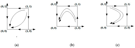
Figure 1.
Strategy evolution diagram based on Proposition 4 (1): (a) scenario (5); (b) scenario (6); (c) scenario (7).
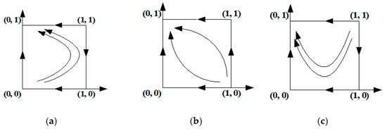
Figure 2.
Strategy evolution diagram based on Proposition 4 (2): (a) scenario (8); (b) scenario (9); (c) scenario (10).
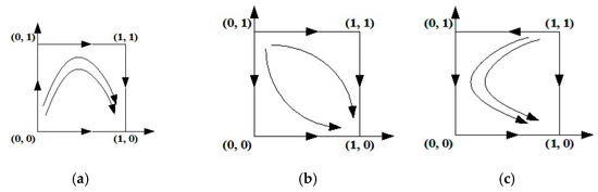
Figure 3.
Strategy evolution diagram based on Proposition 4 (3): (a) scenario (11); (b) scenario (12); (c) scenario (13).
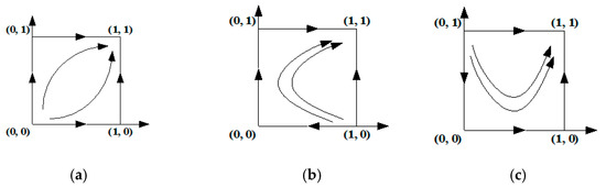
Figure 4.
Strategy evolution diagram based on Proposition 4 (4): (a) scenario (14); (b) scenario (15); (c) scenario (16).
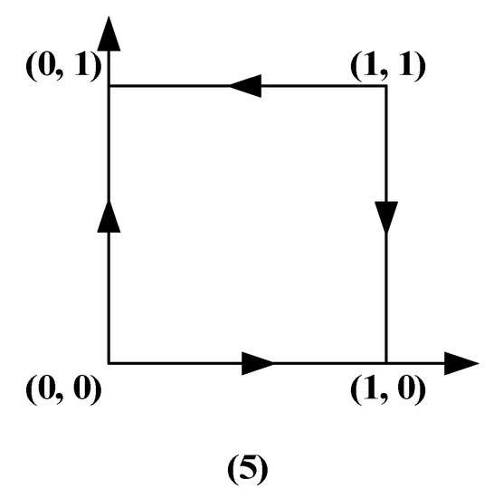
Figure 5.
Strategy evolution diagram based on Proposition 4 (5).
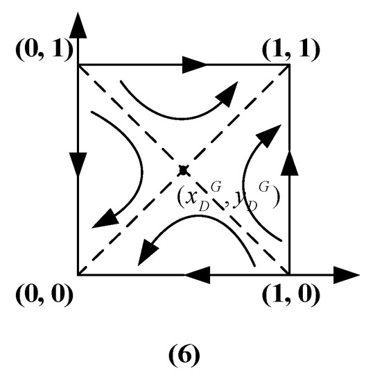
Figure 6.
Strategy evolution diagram based on Proposition 4 (6).
A strategy evolution diagram of enterprises based on Proposition 4 (1) is shown in Figure 1a–c, (0, 0) is the ESS of system (). When both government supervision coefficients and are low, the illegal net income of enterprises is always greater than the loss of basic profit. The negative effect of enterprises choosing URP on their market share is mild, and enterprises have sufficient reason to make an unreasonable price decision in pursuit of additional illegal profit. Therefore, the ESS in this case is to choose URP.
A strategy evolution diagram of enterprises based on Proposition 4 (2) is shown in Figure 2a–c, (0, 1) is the ESS of system (). Government supervision has different effects on large and small enterprises. When and , small enterprises choose URP. In this case, government supervision actually has a weaker deterrent effect on small enterprises than large enterprises. Thus, small enterprises have an incentive to implement unreasonable pricing, while it is unbeneficial for large enterprises to implement unreasonable pricing. According to Proposition 4 (2), we can obtain the following equation:
In Equation (19), indicates the profit and loss (P&L) ratio of small enterprises with the URP strategy, and indicates the P&L ratio of enterprises when both sides choose the URP strategy. Small enterprises can bear the loss of unreasonable pricing decisions, while large enterprises cannot due to reputation damage. In this range of rumor spreading, rumors have a more serious impact on the decisions of small enterprises than on those of large enterprises. Small enterprises focus more on profits and make the URP decision, while large enterprises make the RP decision because they are more concerned with their corporate image that they built over time.
A strategy evolution diagram of enterprises based on Proposition 4 (3) is shown in Figure 3a–c, (1, 0) is the ESS of system (). Government supervision has different effects on large and small enterprises. When and , large enterprises choose URP. Government supervision actually has a weaker deterrent effect on large enterprises than small enterprises. Thus, large enterprises have an incentive to price unreasonably, while it is unbeneficial for small enterprises to price unreasonably. On the basis of Proposition 4 (3), we can obtain the following inequation:
In Equation (20), is the P&L ratio of large enterprises with the URP strategy, and is the P&L ratio of enterprises when both sides choose the URP strategy. Large enterprises can bear the loss of unreasonable pricing decisions, while small enterprises cannot. In this range of rumor spreading, rumors have a more serious impact on the decisions of large enterprises than on the decisions of small enterprises. Large enterprises take the risk of making URP decisions, while small enterprises make RP decisions because they are more vulnerable to the loss of URP decisions.
A strategy evolution diagram of enterprises based on Proposition 4 (4) is shown in Figure 4a–c, (1, 1) is the ESS of system (). When both government supervision coefficients are high, the illegal net income of enterprises is always less than the loss of basic profit. The negative effect of enterprises choosing URP on their market share is significant, and enterprises have no reason to make an unreasonable price decision in pursuit of additional illegal profit. Therefore, in this case, the ESS is to choose RP.
A strategy evolution diagram of enterprises based on Proposition 4 (5) is shown in Figure 5, (0, 1) and (1, 0) are the ESS of system (). One group of enterprises chooses RP when the other group of enterprises has an incentive to choose unreasonable pricing. Thus, the evolutionary stability strategy is that if small enterprises choose URP, large enterprises choose RP, whereas if small enterprises choose RP, large enterprises choose URP.
A strategy evolution diagram of enterprises based on Proposition 4 (6) is shown in Figure 6, (0, 0) and (1, 1) are the ESS of system (), is the saddle point, and (0, 1) and (1, 0) are the unstable points. The ESS of system () is (0, 0) and (1, 1). The ESS and evolutionary process are affected by the initial state of the system (). When the initial state is in regions I and II, the system () converges to (0, 0), and the stability strategy gradually evolves to the prisoner’s dilemma. Finally, the ESS is that enterprises choose unreasonable pricing. When the initial state is in regions III and IV, system () converges to (1, 1), and the stability strategy gradually evolves to Pareto optimality. Finally, the ESS is that enterprises choose RP. Thus, the ESS of system () depends on the area of regions I, II, III and IV.
4.5. Evolutionary Equilibrium Stability Analysis of Proposition 4 (6) via Parameter Variation
We set the sum of the areas of regions I and II as and the sum of the areas of regions III and IV as . The probability of the convergence of the system can be determined based on the proportion of the two regions as follows:
Considering the case of , the following 18 parameters impact the size of the area: and . Then, the following propositions can be obtained.
Proposition 5.
As and increase while the other variations do not change, the size of increases, and the probability that the ESS is (URP, URP) increases. As and increase while the other variations do not change, the size ofdecreases, and the probability that the ESS is (RP, RP) increases.
Proof.
Considering the partial derivatives of with respect to and yields the results shown in Table 7. □
Table 7.
The results of the partial derivatives of .
Proposition 6.
When the proportionis in, regardless of the decision made by large enterprises, small enterprises always choose RP. When the proportionis in, regardless of the decision made by small enterprises make, large enterprises always choose RP.
Proof.
The necessary and sufficient condition for small enterprises to determine whether they choose RP is that when large enterprises choose a mixed game strategy, the expected profits of the small enterprises with the RP strategy are no less than the expected profits of small enterprises with the URP strategy as follows:
Then, we can obtain the following:
Similarly, the necessary and sufficient condition for large enterprises to determine whether they choose RP is as follows:
Proposition 5 shows that when other factors remain unchanged and the conditions of and are satisfied, if basic profit and the additional illegal income of URP increase, the probability that the ESS is (URP, URP) increases. When the basic profit, potential damage and potential income of RP increase, the probability that enterprises choose RP increases. Proposition 6 indicates that to increase the proportion of reasonable pricing, the values of and should be decreased to expand the value range of and , which can encourage enterprises to choose RP. In this situation, the following suggestions could be made by the government: (1) increase the cost of unconscionable pricing, including administrative punishment and publicizing the enterprise’s misconduct; (2) improve the consumer reporting system and open various channels to address consumer complaints; (3) continuously educate customers regarding right-protection awareness; and (4) clarify false rumors in time to stop their spread. □
5. Numerical Simulations
In this section, numerical simulations are conducted in MATLAB to clarify the impacts of different parameters on the ESS. According to previous research and reality, the parameters are set as follows [36]:
, , , , , , , , ; , , , , , , , , ;, , , and .
The evolutionary results are analyzed from three perspectives, i.e., effect of the market environment, the effect of enterprises and effect of governments.
5.1. Effect of the Market Environment on the Game Equilibrium
5.1.1. Effect of Demand Disruption on the Game Equilibrium
When the other factors remain unchanged, the effect of the demand disruption coefficient () on the game is shown in Figure 7a,b. When , the ESS changes from (URP, URP) to (RP, RP). In addition, as increases, the time required for the system to reach (RP, RP) decreases; as decreases, the time required for the system to reach (URP, URP) decreases.
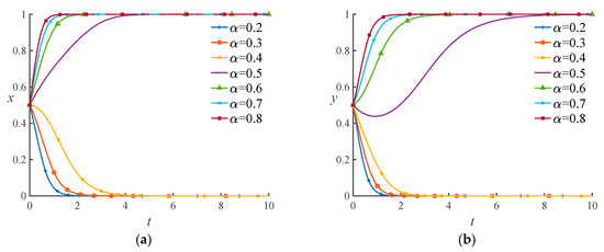
Figure 7.
The effect of on the game equilibrium: (a) small enterprises behavior; (b) large enterprises behavior.
Therefore, when the other factors remain unchanged, if the demand disruption is severe, enterprises are more likely to implement reasonable pricing because the increase in demand disruption offers a greater market share and more profit to those with RP. An enterprise with URP will suffer considerable damage to their basic profit. As a result, the total profit of an enterprise with URP is lower than that of an enterprise with RP. Thus, the optimal strategy of enterprises is RP.
5.1.2. Effect of the Seriousness of Rumor Spreading on the Game Equilibrium
The extent of rumor spreading affects the ESS. The effect of rumor spreading () on the game equilibrium is shown in Figure 8a,b.
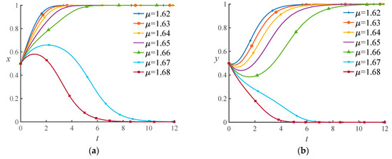
Figure 8.
The effect of on the game equilibrium: (a) small enterprises behavior; (b) large enterprises behavior
According to Figure 8a,b, when , the ESS changes from (RP, RP) to (URP, URP). In addition, as increases, the time required for the system to reach (URP, URP) decreases; as decreases, the time required for the system to reach (RP, RP) decreases.
Therefore, when rumors spread widely, enterprises are more likely to choose unreasonable pricing. In reality, customers are bounded rational, are easily affected by the spread of rumors, and, as a result, begin to hoard supplies. Widespread rumors increase the illegal net income and stimulate enterprises to implement unreasonable pricing. Thus, it is vital for governments to clarify false rumors in time and stop their spreading before such rumors confuse the market.
5.1.3. Joint Influence of Demand Disruption and Rumor Spreading on the Game Equilibrium
The joint influence of and on the game equilibrium is shown in Figure 9a,b. When the other parameters do not change, and change the ESS of the system.
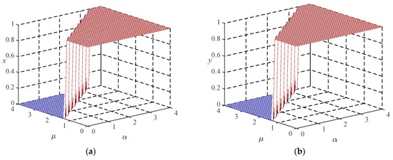
Figure 9.
The effect of and on the game equilibrium: (a) small enterprises behavior; (b) large enterprises behavior.
According to Proposition 5, the criterion determines the ESS. When the criterion is positive, enterprises choose RP; in contrast, when the criterion is negative, enterprises choose URP. In addition, as shown in Figure 9 and the above criterion, (i) when the demand disruption is severe and rumor spreading is mild, the demand disruption plays a leading role in the decision, and enterprises choose RP; (ii) when rumor spreading is severe and the demand disruption is mild, rumors have a stronger effect on the decision, and enterprises choose URP; and (iii) when the rumor spreading and demand disruption are both severe, the demand disruption has a stronger effect on the decision, and enterprises eventually choose RP.
5.2. Effect of Enterprise Responses on the Game Equilibrium
5.2.1. Effect of the Initial Proportion of RP in the Same Group on the Game Equilibrium
The effect of the initial proportion of the market with RP on the game equilibrium is analyzed. When , the effect of on small enterprises’ behavior is shown in Figure 10a, and when , the effect of on large enterprises’ behavior is shown in Figure 10b.
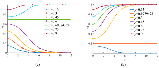
Figure 10.
Effect of and on the game equilibrium: (a) the effect of on small enterprises behavior; (b) the effect of on large enterprises behavior.
According to Figure 10a,b, when the proportions of enterprises choosing RP are 69.38% and 19.79%, respectively, the game achieves the mixed strategy Nash equilibrium. The initial proportion determines the trend of future market evolution. Considering the case of small enterprises, when , the ESS of small enterprises is unreasonable pricing; when , the best choice is RP.
Specifically, when and , the smaller is, the shorter the time required for the system to reach ESS; when , the larger is, the shorter the time required for the system to reach ESS. Similarly, when and , the smaller is, the shorter the time required for the system to reach ESS; when , the larger is, the shorter the time required for the system to reach ESS. Thus, governments should increase the initial proportion of enterprises choosing reasonable pricing to encourage enterprises to choose RP.
According to Proposition 6, when is within , small enterprises choose URP, and when is within , large enterprises choose URP. Therefore, the probability that small enterprises choose URP is larger than that of large enterprises; thus, small enterprises are more likely to overcharge.
5.2.2. Effect of the Proportion of RP in the Other Group on the Game Equilibrium
The mutual effect of large and small enterprise behavior is shown in Figure 11. Figure 11a depicts the impact of large enterprises’ behavior on small enterprises. When the initial proportion of small enterprises that choose RP remains constant, as the proportion of large enterprises that choose RP gradually increases, the final decision of small enterprises converges to RP. Figure 11b depicts the impact of small enterprises’ behaviors on large enterprises. Similarly, when the initial proportion of large enterprises that choose RP remains constant, as the proportion of small enterprises with RP gradually increases, the final decision of large enterprises converges to RP.
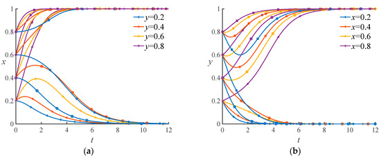
Figure 11.
Effect of the mutual relation between and on the game equilibrium: (a) the effect of on small enterprises behavior; (b) the effect of on large enterprises behavior.
In addition, the impact of large enterprises on small enterprises is shown to be greater than the impact of small enterprises on large enterprises. Thus, the convergence speed of small enterprises affected by large enterprises choosing RP is faster than that of large enterprises affected by small enterprises choosing RP.
5.2.3. Effect of the Potential Income on the Game Equilibrium
To analyse the effect of potential income on enterprises’ RP behavior under demand disruption, when the other parameters do not change, the effects of potential income and on enterprise behavior are shown in Figure 12a,b respectively.
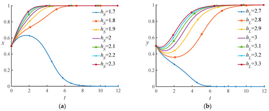
Figure 12.
Effect of and on the game equilibrium: (a) the effect of on small enterprises behavior; (b) the effect of on large enterprises behavior.
Figure 12a shows that when , small enterprises choose URP; when , small enterprises set a reasonable price. In addition, as increases, the time required for small enterprises to reach the ESS of choosing RP decreases. Similarly, Figure 12b shows that when , large enterprises choose URP; when , as increases, the time required for large enterprises to reach the ESS of RP decreases.
5.2.4. Effect of the Additional Illegal Income on the Game Equilibrium
According to Proposition 4 (6), the ESS of the system () is (RP, RP) or (URP, URP). If the ESS of the system () is (RP, RP), the illegal net income of enterprises should be controlled at , , and . When government supervision resources are limited, market changes depend on mutual restraint between enterprises.
The effects of the additional illegal income of small enterprises and on enterprise behavior are shown in Figure 13a,b, and the effects of the additional illegal income of large enterprises and on enterprise behavior are shown in Figure 13c,d.
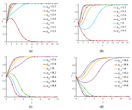
Figure 13.
The effect of and on the game equilibrium: (a) the effect of on small enterprises behavior; (b) the effect of on large enterprises behavior; (c) the effect of on small enterprises behavior; (d) the effect of on large enterprises behavior.
According to Figure 13a,b, when and , enterprises choose RP. Furthermore, as and decrease, the time required for the system to reach the ESS decreases. According to Figure 13c,d, changes in the values of and impact the ESS. When and , enterprises choose RP; when and , enterprises set unreasonable prices to obtain more profit.
The additional illegal income is directly related to the market share; thus, a change in the market share will alter the proportion of unreasonable pricing. The market can be changed in the following two ways: 1. enterprises that set unreasonable prices experience a reduction in their market share and 2. new enterprises enter the market and seize a part of the market share.
5.3. Effect of Government Supervision on the Game Equilibrium
To analyse the effect of government supervision on reducing URP behavior in the market under demand disruption, when the other parameters do not change, the effect of on enterprises’ behavior is shown in Figure 14a. The effect of on enterprises’ behavior is shown in Figure 14b.
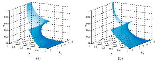
Figure 14.
The effect of and on the game equilibrium: (a) the effect of on small and large enterprises behavior; (b) the effect of on small and large enterprises behavior.
According to Figure 14a,b, when and , both small and large enterprises choose RP. When , both small and large enterprises choose URP; thus, enterprises set unreasonable prices to obtain additional profits. In addition, when and increase, the time required for enterprises to choose RP decreases. When and decrease, the time required for enterprises to choose URP decreases. When and , enterprises choose RP. As increases, the time required for the system to reach the ESS decreases. When , both small and large enterprises choose URP. As decreases, the time required for the system to reach the ESS decreases.
6. Conclusions
Given the situation of rumors and demand disruption, two evolutionary game models of enterprises are developed, i.e., those with a government supervision mechanism and those without a government supervision mechanism. To maintain the stability and sustainability of the market, this study analyses the factors affecting decision behavior and demonstrates the evolutionary paths of participants facing different situations. Finally, the conclusions and managerial insights verified by the numerical simulations are drawn from both theoretical and practical perspectives.
From the exogenous perspective, we draw the following conclusions:
- Demand disruption encourages both large and small enterprises to implement RP. When the demand disruption is severe, the market share of enterprises that choose RP is larger than that of those that choose URP, resulting in a higher profit.
- Rumour spreading disrupts the stability and sustainability of the market. Enterprises have different strategies when facing diverse rumour spreading situations. When rumor spreading is severe, enterprises implement the URP strategy to secure additional illegal profits. In contrast, they adopt the RP strategy to avoid government punishment.
- Two vital factors, i.e., demand disruption and rumour spreading, have opposite effects on enterprises’ decisions. A clear criterion determines the decisive exogenous factor in enterprise decisions. When demand disruption becomes the leading factor in the decision, enterprises choose RP. When rumor spreading has a stronger impact on decisions, enterprises choose URP.
- The government plays an important role in regulating and stabilizing the market; different government supervision strategies guide enterprises to make different decisions. When government supervision is within a particular range, the market has two stability states, i.e., (URP,URP) and (RP,RP). In this case, external factors, such as demand disruption, rumor spreading and government supervision, are vital factors determining enterprise behavior. When government supervision increases to a certain range, all enterprises choose RP. Furthermore, as the intensity of government supervision increases, the required time for enterprises to make RP decisions decreases.
From the endogenous perspective, we draw the following conclusions:
- The comparison between the P&L ratio of URP and rumour spreading is a key endogenous factor in decisions. When the P&L ratio of URP is greater than the seriousness of rumor spreading, enterprises are not sensitive to rumors and, thus, choose RP. In contrast, when the P&L ratio of URP is smaller than the seriousness of rumor spreading, enterprises are easily swayed by rumors and make the decision to implement URP. Moreover, if the P&L ratio of enterprises in the situation that both sides choose URP is larger than the seriousness of rumor spreading, enterprises will choose URP asynchronously.
- The proportion of RP determines the trend of future market evolution. When the proportion of small enterprises choosing RP is within , all small enterprises eventually make reasonable pricing decisions. When the proportion of large enterprises choosing RP is within , all large enterprises eventually make reasonable pricing decisions.
- The decisions of small and large enterprises have mutual effects on each other. A higher proportion of larger enterprises with RP will impact small enterprises’ decisions to ultimately engage in reasonable pricing; a higher proportion of small enterprises with RP will motivate large enterprises to eventually choose reasonable pricing. The impact of large enterprises on small ones is greater than that of small enterprises on large ones.
- The market share of an enterprise impacts the enterprise’s decisions. Small enterprises with a small market share are more concerned about profit and are more likely to choose URP, while large enterprises with a large market share are concerned with their corporate image and are more likely to choose RP.
Several practical suggestions can be made. For governments, promotions of the importance of corporate image and public education concerning consumer rights and interest awareness could prevent market disorders when emergencies occur. The government should pay more attention to correctly identifying the cause of demand disruption, clarifying false rumors and stopping their spread in time. Given their limited resources, governments should exert different levels of effort to regulate the market according to the seriousness of the demand disruption and rumor spreading. The government should apply a prioritized supervision strategy to small businesses when rumor spreading is serious. For enterprises, a price strategy could be made according to whether they value profit over corporate image or vice versa. The P&L ratio can help enterprises forecast the outcome of their pricing choices. Furthermore, the initial probability of RP and the decisions of other enterprises could help them become aware of market evolution, thus assisting them in making better choices.
This study has two limitations that should be resolved in future research. First, small and large enterprises constitute the two homogeneous game participants considered in this paper; future research should investigate vertical games with participation by the government, enterprises and customers. Second, demand disruption and rumor spreading are discussed separately in this paper; future research should further investigate the effect of rumor-caused demand disruption on enterprise behavior.
Author Contributions
Methodology, C.Z.; software, C.Z.; writing—original draft preparation, L.L.; writing—review and editing, C.Z. and H.S.; supervision, H.S.; final manuscript preparation, H.Y. All authors have read and agreed to the published version of the manuscript.
Funding
This work was funded by the National Natural Science Foundation of China (No. 71901004), Beijing Philosophy and Social Science Project (No. 18GLC085) and National Natural Science Foundation of China (No. 71871002).
Informed Consent Statement
Informed consent was obtained from all subjects involved in the study.
Data Availability Statement
The data presented in this study are available in Zhang et al. [36].
Conflicts of Interest
The authors have no conflicts of interest to declare.
Appendix A
Appendix B
The trace condition () and determinant value () are then calculated:
Appendix C
Appendix D
The trace condition () and determinant value () are calculated:
Appendix E
According to Table A1, when or or , i.e., , , the ESS is (URP, URP);
Table A1.
The ESS of the system ( ) in Proposition 4 (1).
Table A1.
The ESS of the system ( ) in Proposition 4 (1).
| Stable Point | scenario (5) | scenario (6) | scenario (7) | ||||||
|---|---|---|---|---|---|---|---|---|---|
| Result | Result | Result | |||||||
| (0, 0) | + | - | ESS | + | - | ESS | + | - | ESS |
| (0, 1) | - | ? | Saddle point | - | ? | Saddle point | + | + | Unstable point |
| (1, 0) | - | ? | Saddle point | + | + | Unstable point | - | ? | Saddle point |
| (1, 1) | + | + | Unstable point | - | ? | Saddle point | - | ? | Saddle point |
According to Table A2, when or or , i.e., , , the ESS is (URP, RP);
Table A2.
The ESS of the system ( ) in Proposition 4 (2).
Table A2.
The ESS of the system ( ) in Proposition 4 (2).
| Stable Point | scenario (8) | scenario (9) | scenario (10) | ||||||
|---|---|---|---|---|---|---|---|---|---|
| Result | Result | Result | |||||||
| (0, 0) | + | + | Unstable point | - | ? | Saddle point | - | ? | Saddle point |
| (0, 1) | + | - | ESS | + | - | ESS | + | - | ESS |
| (1, 0) | - | ? | Saddle point | + | + | Unstable point | - | ? | Saddle point |
| (1, 1) | - | ? | Saddle point | - | ? | Saddle point | + | + | Unstable point |
According to Table A3, when or or , i.e., , , the ESS is (RP, URP);
Table A3.
The ESS of the system ( ) in Proposition 4 (3).
Table A3.
The ESS of the system ( ) in Proposition 4 (3).
| Stable Point | scenario (11) | scenario (12) | scenario (13) | ||||||
|---|---|---|---|---|---|---|---|---|---|
| Result | Result | Result | |||||||
| (0, 0) | + | + | Unstable point | - | ? | Saddle point | - | ? | Saddle point |
| (0, 1) | - | ? | Saddle point | + | + | Unstable point | - | ? | Saddle point |
| (1, 0) | + | - | ESS | + | - | ESS | + | - | ESS |
| (1, 1) | - | ? | Saddle point | - | ? | Saddle point | + | + | Unstable point |
According to Table A4, when or or , i.e., and , the ESS is (RP, RP);
Table A4.
The ESS of the system ( ) in Proposition 4 (4).
Table A4.
The ESS of the system ( ) in Proposition 4 (4).
| Stable Point | scenario (14) | scenario (15) | scenario (16) | ||||||
|---|---|---|---|---|---|---|---|---|---|
| Result | Result | Result | |||||||
| (0, 0) | + | + | Unstable point | - | ? | Saddle point | - | ? | Saddle point |
| (0, 1) | - | ? | Saddle point | - | ? | Saddle point | + | + | Unstable point |
| (1, 0) | - | ? | Saddle point | + | + | Unstable point | - | ? | Saddle point |
| (1, 1) | + | - | ESS | + | - | ESS | + | - | ESS |
According to Table A5, when , i.e., and , the ESS is (RP, URP) or (URP, RP);
Table A5.
The ESS of the system ( ) in Proposition 4 (5).
Table A5.
The ESS of the system ( ) in Proposition 4 (5).
| Stable Point | Result | |||
|---|---|---|---|---|
| scenario (17) | (0, 0) | + | + | Unstable point |
| (0, 1) | + | - | ESS | |
| (1, 0) | + | - | ESS | |
| (1, 1) | + | + | Unstable point |
According to Table A6, when , i.e., and , the ESS is (URP, URP) or (RP, RP).
Table A6.
The ESS of the system ( ) in Proposition 4 (6).
Table A6.
The ESS of the system ( ) in Proposition 4 (6).
| Stable Point | Result | |||
|---|---|---|---|---|
| scenario (18) | (0, 0) | + | - | ESS |
| (0, 1) | + | + | Unstable point | |
| (1, 0) | + | + | Unstable point | |
| (1, 1) | + | - | ESS | |
| - | 0 | Saddle point |
References
- Li, M.; Zhang, H.; Georgescu, P. The stochastic evolution of a rumor spreading model with two distinct spread inhibiting and attitude adjusting mechanisms in a homogeneous social network. Phys. A 2021, 562, 125321. [Google Scholar] [CrossRef] [PubMed]
- Yin, H.; Wang, Z.; Gou, Y. Rumor Diffusion and Control Based on Double-Layer Dynamic Evolution Model. IEEE Access 2020, 8, 115273–115286. [Google Scholar] [CrossRef]
- Qi, X.; Jonathan, F.; Yu, G. Supply chain coordination with demand disruptions. Omega 2004, 32, 301–312. [Google Scholar] [CrossRef]
- Choi, T. Impacts of retailer’s risk averse behaviors on quick response fashion supply chain systems. Ann. Oper. Res. 2016, 286, 239–257. [Google Scholar] [CrossRef]
- Hunt, S. Sustainable marketing, equity, and economic growth: A resource-advantage, economic freedom approach. J. Acad. Mark. Sci. 2011, 39, 7–20. [Google Scholar] [CrossRef]
- Sun, Y.; Kim, K.; Kim, J. Examining relationships among sustainable orientation, perceived sustainable marketing performance, and customer equity in fast fashion industry. J. Glob. Fash. Mark. 2014, 5, 74–86. [Google Scholar] [CrossRef]
- Zhao, H.; Lin, B.; Guo, C. A mathematics model for quantitative analysis of demand disruption caused by rumor spreading. Int. J. Inf. Technol. Decis. Mak. 2014, 13, 585–602. [Google Scholar] [CrossRef]
- Chen, Z.; Teng, C.; Zhang, D.; Sun, J. Modelling inter-supply chain competition with resource limitation and demand disruption. Int. J. Syst. Sci. 2014, 47, 1644–1658. [Google Scholar] [CrossRef]
- Yan, B.; Jin, Z.; Liu, Y.; Yang, J. Decision on risk-averse dual-channel supply chain under demand disruption. Commun. Nonlinear Sci. Numer. Simul. 2018, 55, 206–224. [Google Scholar] [CrossRef]
- Xu, M.; Qi, X.; Yu, G.; Zhang, H.; Gao, C. The demand disruption management problem for a supply chain system with nonlinear demand functions. J. Syst. Sci. Syst. Eng. 2003, 12, 82–97. [Google Scholar] [CrossRef]
- Chen, K.; Xiao, T. Demand disruption and coordination of the supply chain with a dominant retailer. Eur. J. Oper. Res. 2009, 197, 225–234. [Google Scholar] [CrossRef]
- Han, J.; Shin, K. Evaluation mechanism for structural robustness of supply chain considering disruption propagation. Int. J. Prod. Res. 2015, 54, 135–151. [Google Scholar] [CrossRef]
- Ali, S.; Rahman, M.; Tumpa, T.; Rifat, A.M.; Paul, S. Examining price and service competition among retailers in a supply chain under potential demand disruption. J. Retail. Consum. Serv. 2018, 40, 40–47. [Google Scholar] [CrossRef]
- Yang, L.; Li, Z.; Giua, A. Containment of rumor spread in complex social networks. Inf. Sci. 2020, 506, 113–130. [Google Scholar] [CrossRef]
- Kim, S.; Kim, S. Impact of the Fukushima Nuclear Accident on Belief in Rumors: The Role of Risk Perception and Communication. Sustainability 2017, 9, 2188. [Google Scholar] [CrossRef]
- Zhao, L.; Wang, X.; Wang, J.; Qiu, X.; Xie, W. Rumor-Propagation Model with Consideration of Refutation Mechanism in Homogeneous Social Networks. Discret. Dyn. Nat. Soc. 2014, 5, 1–11. [Google Scholar] [CrossRef]
- Zhang, Y.; Su, Y.; Li, W.; Liu, H. Modeling rumor propagation and refutation with time effect in online social networks. Int. J. Mod. Phys. C 2018, 29, 1850068. [Google Scholar] [CrossRef]
- Xiao, Y.; Chen, D.; Wei, S.; Li, Q.; Wang, H.; Xu, M. Rumor propagation dynamic model based on evolutionary game and anti-rumor. Nonlinear Dyn. 2018, 95, 523–539. [Google Scholar] [CrossRef]
- Liu, F.; Li, M. A game theory-based network rumor spreading model: Based on game experiments. Int. J. Mach. Learn. Cybern. 2019, 10, 1449–1457. [Google Scholar] [CrossRef]
- Indu, V.; Thampi, M. A nature—inspired approach based on Forest Fire model for modeling rumor propagation in social networks. J. Netw. Comput. Appl. 2019, 125, 28–41. [Google Scholar] [CrossRef]
- Lodree, E., Jr.; Taskin, S. An insurance risk management framework for disaster relief and supply chain disruption inventory planning. J. Oper. Res. Soc. 2008, 59, 674–684. [Google Scholar] [CrossRef]
- Kitamuraa, T.; Managib, S. Energy security and potential supply disruption: A case study in Japan. Energy Policy 2017, 110, 90–104. [Google Scholar] [CrossRef]
- Zhao, L.; Wang, C.; Gu, H.; Yue, C. Market incentive, government regulation and the behavior of pesticide application of vegetable farmers in China. Food Control. 2018, 85, 308–317. [Google Scholar] [CrossRef]
- Zhang, N.; Zhang, X.; Yang, Y. The behavior mechanism of the urban Joint distribution alliance under government supervision from the perspective of sustainable development. Sustainability 2019, 11, 6232. [Google Scholar] [CrossRef]
- Zhang, N.; Yang, Y.; Wang, X. Game Analysis on the Evolution of Decision-Making of Vaccine Manufacturing Enterprises under the Government Regula-tion Model. Vaccines 2020, 8, 267. [Google Scholar] [CrossRef]
- Hao, C.; Du, Q.; Huang, Y. Evolutionary Game Analysis on Knowledge-Sharing Behavior in the Construction Supply Chain. Sustainability 2019, 11, 5319. [Google Scholar] [CrossRef]
- Sun, H.; Wan, Y.; Lv, H. System Dynamics Model for the Evolutionary Behaviour of Government Enterprises and Consumers in China’s New Energy Vehicle Market. Sustainability 2020, 12, 1578. [Google Scholar] [CrossRef]
- Chen, W.; Hu, Z. Analysis of Multi-Stakeholders’ Behavioral Strategies Considering Public Participation under Carbon Taxes and Subsidies: An Evolutionary Game Approach. Sustainability 2020, 12, 1023. [Google Scholar] [CrossRef]
- Tian, Y.; Govindan, K.; Zhu, Q. A system dynamics model based on evolutionary game theory for green supply chain management diffusion among Chinese manufacturers. J. Clean. Prod. 2014, 80, 96–105. [Google Scholar] [CrossRef]
- Mojgan, A.; Behrouz, T.; Mohammad, H. An evolutionary game model for analysis of rumor propagation and control in social networks. Phys. A 2019, 523, 21–39. [Google Scholar]
- Sun, H.; Wan, Y.; Zhang, L.; Zhou, Z. Evolutionary game of the green investment in a two-echelon supply chain under a government subsidy mechanism. J. Clean. Prod. 2019, 235, 1315–1326. [Google Scholar] [CrossRef]
- Kang, K.; Zhao, Y.; Zhang, J.; Qiang, C. Evolutionary game theoretic analysis on low-carbon strategy for supply chain enterprises. J. Clean. Prod. 2019, 230, 981–994. [Google Scholar] [CrossRef]
- Xiao, T.; Yu, G. Supply chain disruption management and evolutionarily stable strategies of retailers in the quantity-setting duopoly situation with homogeneous goods. Eur. J. Oper. Res. 2006, 173, 648–668. [Google Scholar] [CrossRef] [PubMed]
- Friedman, D. Evolutionary games in economics. Econometrica 1991, 59, 637–666. [Google Scholar] [CrossRef]
- Xu, J.; Cao, J.; Wang, Y. Evolutionary game on government regulation and green supply chain decision-making. Energies 2020, 13, 620. [Google Scholar] [CrossRef]
- Zhang, W.; Fu, J.; Li, H. Coordination of supply chain with a revenue-sharing contract under demand disruptions when retailers compete. Int. J. Prod. Econ. 2012, 138, 68–75. [Google Scholar] [CrossRef]


Publisher’s Note: MDPI stays neutral with regard to jurisdictional claims in published maps and institutional affiliations. |
© 2021 by the authors. Licensee MDPI, Basel, Switzerland. This article is an open access article distributed under the terms and conditions of the Creative Commons Attribution (CC BY) license (http://creativecommons.org/licenses/by/4.0/).