The Calibration of Evaporation Models against the Penman–Monteith Equation on Lake Most

Abstract

Evaporation is one of the main components of the water cycle in nature. Our interest in free water surface evaporation is due to the needs of ongoing hydric recultivation of the former Ležáky–Most quarry, i.e., Lake Most, and also other planned hydric recultivations in the region. One of the key components of hydric reclamation planning is the securitization of long-term sustainability, which is based on the capability to keep the final water level at a stable level. In our work, we are interested in the evaporation estimation in the area of Lake Most (Czech Republic, Europe). This lake has been artificially created only a few years ago, and nowadays we are looking for a simple evaporation model, based on which we will be able to decide which measurement devices have to be installed at the location to provide more localized data to the model. In this paper, we calibrate state-of-the-art simplified evaporation models against the Penman–Monteith equation based on the Nash–Sutcliffe efficiency maximization. We discuss the suitability of this approach using real-world climate data from the weather station located one km from the area of interest.

1. Introduction

Although evaporation is one of the main components of the water cycle in nature—it is reported that it makes up almost two-thirds of continental precipitation—its measurement or calculation procedures are complicated and burdened with a high degree of uncertainty. The measurement is provided by evaporation pans and class A is widely adopted as the standard pan. An investigation of the uncertainty of such measurement provided in [1] assumed its precision to be ±0.1 mm. According to the study in [2], the results of monthly evaporation obtained from two pans at the same locations could vary by up to $4\%$ and the influence of an installed bird guard fence was estimated to be $7\%$. The guidelines detailed in [3] suggested that water turbidity could cause measurements errors of up to $5\%$. The uncertainty in computed estimates is due to the complexity of evaporation as a physical phenomenon and several factors that affect this process. Traditionally (see [4]), computational methods are divided into two classes, namely aerodynamic formulae and energy budget formulae. However, this classification is quite rough and in practice it is hard to distinguish mass transfer factors from energy budget ones. 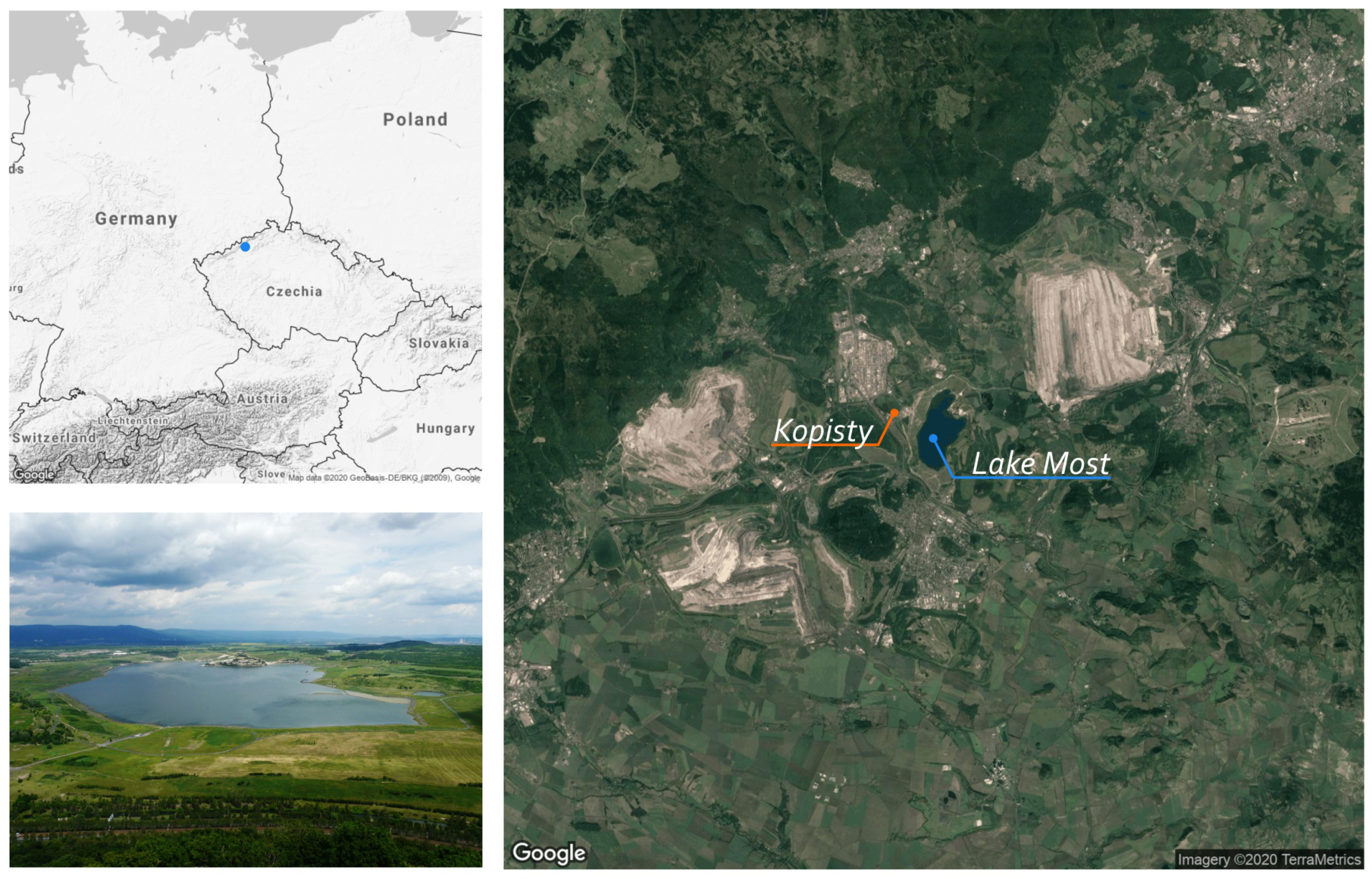Based on meteorological data needed to compute evaporation estimates, the methods could be classified as temperature-based, radiation-based, mass transfer-based and combination methods [5,6]. Furthermore, it is important to note that fumes occur both from the free water level and from the Earth’s surface, and these processes need to be distinguished. The above stated then leads to the introduction of terms such as evaporation, transpiration, or evapotranspiration. We also distinguish whether we are considering a potential (possible) or actual (real) evaporation rate. Both computational methods and measurement methods deal with potential values, which in both cases is because there is an effort to simplify the description. The goal of this work is to deal with the inaccuracy of computed results and their relation with inaccuracy in the measurement of physical quantities influencing evaporation. The interest in such improvements of free water surface evaporation is due to the needs of the ongoing hydric recultivation of the former Ležáky–Most quarry, i.e., Lake Most (the Czech Republic, central Europe, 50°32′13′′ N 13°38′40′′ E), and also other planned hydric recultivations in the region. One of the key components of the hydric reclamation planning is the securitization of long-term sustainability, which is based on the capability to keep the final water level at a stable level. In this context, note that the usual approach to the water management of pit lakes is to estimate evaporation using pan coefficient modeling with floating pans. Additionally, the water temperature or the water temperature profile are monitored. Usage of such equipment and observation could lead to significant improvements of evaporation estimates. In [7], a correction of underestimations by $20\%$ was reported. However this approach is not applicable in the case of currently planned reclamation since open cut mining operations are still in progress there.

Evaporation influences the global climate and, consequently, each of the areas of human activity, which is manifested by increased interest in the field of its modeling. In the conditions of climate change, this task is even more challenging and water resources’ management needs accurate methods providing water loss estimates. In [8], a comparison of combined, water balance and pan evaporation techniques’ performance was undertaken and the Penman–Monteith model with local site data was recommended. Similarly, a study of a drying urban lake—Sukhna Lake in northern India—provided in [9], suggested site-specific observation for each hydrologic process. On the other hand, the influence of water dams and reservoirs on agriculture or municipality life was monitored too. An analysis done in [10] showed that construction of small dams together with their proper management could lead to an increase in crop yield in targeted area. The research in [11] presents a representative example of water management in northern Greece. All papers cited here emphasized the work with local conditions and needs.

As mentioned above, the methods of calculating the rate of evaporation according to the inputs used can be divided into several groups. Most commonly, the division into models of temperature, radiation, mass transfer, and combined methods is used. This wide range of methods reflects the long process of their development, which began with Dalton’s work in the early 19th century, continued with the classic Penman paper [12], and developed further in the 1990s, when the aforementioned quantity of used methods led the Food and Agriculture Organization (FAO) of the United Nations to work towards determining the most appropriate method, or at a least reference method, that could be used in the widest possible range of cases under investigation. The collaborative work and consultation of FAO experts yielded guidelines for computing evapotranspiration [3].

The analysis of the performance of the various calculation methods reveals the need for formulating a standard method for the computation of evapotranspiration [3]. The Penman–Monteith method (FAO) is recommended as the sole standard method. It is a method with a strong likelihood of correctly predicting the evapotranspiration in a wide range of locations and climates with differing local factors. These include solar radiation, sunshine duration, wind speed, air humidity, air temperature, and properties of the observing station/s location [13,14,15]. The FAO has provisions for the application of the method in data-poor situations. The use of older FAO or other reference evapotranspiration methods is no longer encouraged [16,17].

In this paper, we aim to simplify the FAO equation in terms of the number of input quantities. In Section 2, we shortly review this equation and introduce all the required data for the computation of evaporation estimation. This section also includes the presentation of other selected models, which are not considered by FAO to be a standard; however, they are less complex. Our goal is to use these simpler models to model the evaporation in the area of Lake Most (see Section 2.8 for area description) by calibrating the parameters of models in the fitting optimization process against the evaporation estimation by FAO. This calibration process is described in Section 2.7. The motivation came from the lack of measuring devices in direct vicinity to the lake. Section 2.9 demonstrates the necessity of the presence of measuring devices as close as possible to the area of interest; even a small change in the measured climate data can cause the overestimation of evaporation.

In our approach, the data that we provide to the FAO equation are measured in the Kopisty weather station (located approximately 1 km from Lake Most; see Section 2.9 for details). This distance is sufficient for providing the approximation of climate data in a wider area including Lake Most; however, the FAO equation is sensitive in terms of input data.

The construction of a new weather station with all measuring devices necessary for FAO right next to the lake does not make any sense (because the Kopisty station is only 1 km away); therefore, the simplified model with a smaller amount of input data should be used.

Our research will be used as a background for the decision process for the installation of specific measuring devices in the area for obtaining data for the simpler calibrated model. See Section 3 for our results and Section 4 for the discussion.

Finally, Section 5 concludes the paper. We believe that the presented calibration methodology can be used as a general tool for solving problems with similar input situations: the climate measuring devices are located in a wider range of the area of interest and the problem is to decide which measuring devices should be installed directly at the location to provide a better (and cheaper) evaporation estimation.

2. Materials and Methods

The FAO Penman–Monteith equation [3] is given by:

$$E_{\mathrm{FAO}}=\frac{0.408\Delta (R_n-G)+\gamma \frac{900}{T_a+273}{u}_2(e_s-e_a)}{\Delta +\gamma (1+0.34u_2)}$$

(1)

where $E_{\mathrm{FAO}}$ is the intensity of evapotranspiration (kg · m${}^{-2}$· s${}^{-1}$), $\Delta$ is the derivative of the saturated water vapor pressure with respect to the air temperature (kPa · °C${}^{-1}$), $R_n$ is the radiation balance on the surface (kJ · m${}^{-2}$· s${}^{-1}$), G is the heat flow in the soil (kJ · m${}^{-2}$· s${}^{-1}$) (e.g., for the water surface $G=0$ [18]), $e_s$ is the saturated water vapor pressure in the air temperature (kPa), $e_a$ is the current water vapor pressure (kPa) (the difference $e_s-e_a$ is called the saturation supplement), $\gamma$ is the psychrometric constant (m · s${}^{-1}$) (e.g., if the air temperature is measured in °C and the water vapor pressure is measured in $mb$ or kPa, then $\gamma =0.66$), $T_a$ is the average air temperature (°C), and $u_2$ is the air speed measured at the height of 2 m (m · s${}^{-1}$).

At first glance, it is evident that this is a very complicated relationship; for ordinary users or laypeople it is even possible to talk about a relationship incomprehensible or ungraspable.

Thus several different equations for evaporation estimation appear in the technical literature, which deals with finding relationships that are less complicated and computationally less demanding. However, Equation (1) can still be taken as a standard to which the results of other methods can be related.

In this paper, we deal with the following equations, selected to represent the entire variety of usual approaches, i.e., temperature, radiation, mass-transfer, and combined methods.

We shortly review the Šermer equation [19], the Beran–Vizina equation [20], the Hargreaves–Samani equation [21], the Schendel equation [22], the Priestley–Taylor equation [23], the Kharrufa equation [24], and the VUV equation [20].

Some of these equations can produce negative evaporation values. The typical approach is to map all negative values to zero. In our computations, we follow this standard.

2.1. Šermer Equation and Beran–Vizina Equation

These equations are commonly used in the Czech Republic. They are derived using the regression between observed/measured vapor and daily mean air temperature. The regression is used to find both the linear and exponential models. The following equations can be found in [20], where the authors compare them against the measurement performed by a 20 m${}^2$ vapor meter in the weather station in Hlasivo located in the South Bohemian Region.

The Šermer equation [19] is given by:

$$E_{\mathrm{S}}={10}^{0.0452T_a-0.204}$$

(2)

and the Beran–Vizina [20] equation is given by:

$$E_{\mathrm{BV}}=0.2157T_a+1.1133.$$

(3)

In the equations, the amount of vapor is measured in mm · d${}^{-1}$ and $T_a$ denotes the daily mean air temperature measured in °C. Equations (2) and (3) have been recently compared (see [25]).

Equation (2) has a form of an exponential function, and therefore the results attain only non-negative values. On the other hand, in the case of Equation (3), the value of $E_{\mathrm{BV}}\ge 0$ is defined only for days with an average temperature lower than $-0.526$ °C, since otherwise, the vapor $E_{\mathrm{BV}}$ would attain negative values.

In the case of $E_{\mathrm{BV}}$, a value of zero vapor (without the computation) was determined in 163 cases during the whole monitored period of 2014–2019, i.e., in average 27 days per year. However, it is necessary to mention that, for instance, during the year 2018, which had an average temperature of 10.8 °C, there was also the largest number of days with an average temperature below freezing, namely 48 days.

During the calibration process, we suppose the constants in (2) and (3) to be (unknown) coefficients. We get the parametric models:

$$E_{\mathrm{S}}\left(\theta \right)={10}^{{\theta }_1{T}_a+{\theta }_2}$$

(4)

and

$$E_{\mathrm{BV}}\left(\theta \right)=max\left\{0,{\theta }_1{T}_a+{\theta }_2,\right\}$$

(5)

where $\theta \in {\mathbb{R}}^2$ are the parameters of the models that should be optimized.

In the case of (5), we used the maximum to ensure the non-negativity of the evaporation modeled by the parametric model.

2.2. Hargreaves–Samani Equation

This method was proposed by Hargreaves in [26] and gradually extended into its final form as presented in [21]. Usually, the Hargreaves–Samani equation is presented in the following form:

$$E_{\mathrm{HS}}=0.0023R_a\sqrt{T_r}(T_a+17.8),$$

(6)

where $T_a$ denotes the average air temperature (°C), $T_r$ is the difference between the maximal and minimal air temperature during the reporting period (°C), and $R_a$ denotes the extraterrestrial radiation.

Although Equation (6) includes the radiation term $R_a$, the model is classified as a temperature equation. The reason is that this term denotes only the theoretical value and is computed using the following formula:

$$R_a=\frac{24\times 60}{\pi }{G}_{SC}{d}_r\left({\omega }_{S}sin\left(\phi \right)sin\left(\delta \right)+sin{\omega }_{S}cos\left(\phi \right)cos\left(\delta \right)\right).$$

Please note that this equation is based only on the latitude of the considered area $\phi$ and the solar declination $\delta$ determined by the serial number of the day of the year.

Extraterrestrial radiation $R_a$ is measured in MJ · m${}^{-2}$· g${}^{-1}$. For obtaining the result $E_{\mathrm{HS}}$ in millimeters per day, it is necessary to divide the value of $R_a$ by the value of the water-specific heat capacity $\lambda$ = 2.45 MJ · kg${}^{-1}$. Consequently, the Hargreaves–Samani equation can be found in several equivalent forms:

$$E_{\mathrm{HS}}=\left\{\begin{array}{c}0.0023\frac{R_a}{2.45}(T_a+17.8)\sqrt{T_r}\hfill \\ 0.0023\left(0.408R_a\right)(T_a+17.8)\sqrt{T_r}\hfill \\ 0.00094R_a(T_a+17.8)\sqrt{T_r}.\hfill \end{array}\right.$$

(7)

In this paper, we write the parametric form of the Hargreaves–Samani equation:

$$E_{\mathrm{HS}}\left(\theta \right)=max\left\{0,\frac{{\theta }_1{R}_a(T_a+{\theta }_2)\sqrt{T_r}}{\lambda }\right\}$$

(8)

with parameters $\theta \in {\mathbb{R}}^2$. These parameters will be optimized during the calibration process.

2.3. Schendel Equation

In the previous equations, the computation of the rate of evaporation is based on the measurement of the air temperature. In the case of the Schendel equation, one has to also provide the measurements of the relative humidity $RH$. The equation has a simple form and it can be found in the original paper by Schendel [22] and also in later publications, e.g., [27,28]. The model is given by:

$$E_{\mathrm{Sch}}=16\frac{T_a}{RH}.$$

(9)

The Schendel equation can be written in parametric form:

$$E_{\mathrm{Sch}}\left(\theta \right)=max\left\{0,{\theta }_1\frac{T_a}{RH}\right\}$$

(10)

with unknown parameter $\theta \in \mathbb{R}$.

2.4. Priestley–Taylor Equation

A potential evapotranspiration based on the Priestley–Taylor can be considered as a combined method, which is developed as a combination of the turbulent diffusion method and the method of energy balance [23]. The basic equation for the computation of the potential evapotranspiration by the Priestley–Taylor method is given by:

$$E_{\mathrm{PT}}=\frac{1.26\Delta (R_n-G)}{\lambda (\Delta +\gamma )}$$

(11)

where $\Delta$ is the derivative of the saturated water vapor pressure with respect to the air temperature (kPa · °C${}^{-1}$). Additionally, $R_n$ is the radiation flow intensity measured in W · m${}^{-2}$, G is the heat flow intensity at the water surface level (W · m${}^{-2}$), $\gamma$ is the psychrometric constant measured in kPa · °C${}^{-1}$, and $\lambda$ = 2.45 MJ · kg${}^{-1}$ is the value of the water-specific heat capacity.

In this paper, we optimize the constant parameter in Equation (11), i.e., we consider a parametric model:

$$E_{\mathrm{PT}}\left(\theta \right)=max\left\{0,\frac{{\theta }_1\Delta (R_n-G)}{\lambda (\Delta +\gamma )}\right\},$$

(12)

where $\theta \in \mathbb{R}$ is unknown parameter.

2.5. Kharrufa Equation

For arid areas, Kharrufa [24] published a simple equation:

$$E_{\mathrm{K}}=0.34p{T}_a^{1.3},$$

(13)

where p is the percentage of total daytime hours for the period used (daily or monthly) out of total daytime hours of the year. This equation has also been used in a large model comparison [25].

In the parametric form, we deal with zero evaporation in the case of negative temperature $T_a$ and define:

$$E_{\mathrm{K}}\left(\theta \right)=\left\{\begin{array}{cc}0\hfill & \mathrm{if}{T}_a>0,\hfill \\ {\theta }_{1}p{T}_a^{{\theta }_2}\hfill & \mathrm{if}{T}_a\le 0,\hfill \end{array}\right.$$

(14)

where $\theta \in {\mathbb{R}}^2$ are unknown parameters.

2.6. VUV

This formula is presented in the official report Model průběhu meteorologických veličin pro oblast jezera Most do roku 2050 (The modelling of the course of meteorological quantities for Lake Most area until 2050) by Adam Beran from Výzkumný ústav vodohospodářský T. G. Masaryka (VUV, T. G. Masaryk Water Research Institute):

$$E_{\mathrm{VUV}}=0.2157T_a+0.726u_2-1.2259.$$

(15)

All variables in this equation have already been introduced in this paper. This equation has also been used in a large model comparison [25].

The equation can be written in parametric form as:

$$E_{\mathrm{VUV}}\left(\theta \right)=max\left\{0,{\theta }_1{T}_a+{\theta }_2{u}_2+{\theta }_3\right\},$$

(16)

where $\theta \in {\mathbb{R}}^3$ is a vector of unknown parameters.

2.7. The Calibration Process

We optimize the parameters of the models presented in Section 2 against the Penman–Monteith Equation (1). The difference between the models is measured according to the standard Nash–Sutcliffe efficiency (NSE) introduced in [29] as an analogy to the coefficient of determination, and is given by:

$$\mathrm{NSE}(E_{\mathrm{FAO}},E)=1-\left[\frac{{\displaystyle \sum _{t=1}^T}{\left(E_{\mathrm{FAO}}\langle t\rangle -E\langle t\rangle \right)}^2}{{\displaystyle \sum _{t=1}^T}{\left(E_{\mathrm{FAO}}\langle t\rangle -{\stackrel{—}{E}}_{\mathrm{FAO}}\right)}^2}\right],$$

(17)

where $E\langle t\rangle$ is a value of the model in time (day) $t=1,\cdots ,T$, and ${\stackrel{—}{E}}_{\mathrm{FAO}}$ is a mean value of the Penman–Monteith model given by:

$${\stackrel{—}{E}}_{\mathrm{FAO}}=\frac{1}{T}\sum _{t=1}^T{E}_{\mathrm{FAO}}\langle t\rangle .$$

The optimal parameters solve the optimization problem:

$${\theta }^{*}=arg\underset{\theta }{max}\mathrm{NSE}(E_{\mathrm{FAO}},E\left(\theta \right))$$

(18)

where E is any of the parametric models presented in Section 2.

The NSE measures the difference between models in the following way: if the variance between models is equal to zero, then the NSE is equal to one. Conversely, if one model produces a variance equal to the variance of the second one, then it results in an NSE of zero. Practically, $NSE=0$ indicates that the models have the same predictive skill as ${\overline{E}}_{\mathrm{FAO}}$ in terms of the sum of the squared error. For the application of NSE in regression, the NSE is equivalent to the coefficient of determination and it ranges between 0 and 1, and in general, a model is satisfactory if $NSE>0.5$, see [30].

The Nash–Sutcliffe efficiency is widely used in different branches of hydrology, e.g., in [31,32] NSE was used to evaluate performance of hydrological and hydraulic models of flash-floods.

Similarly to our work, in an evaporation study of Lake Van [33], NSE was applied as a comparative criterion of assorted computational methods and the Bowen ratio energy budget method and furthermore was used to choose the best-fit and reasonably accurate model. Also in [34], the open-water evaporation estimate method was recommended based on an analysis of NSE.

Finally, NSE could support the choice of a suitable replacement for the FAO Penman–Monteith potential evapotranspiration estimates in case of insufficient meteorological data. That was the aim of study [35], where three radiation-based and five temperature-based methods were compared with the estimates given by the FAO Penman–Monteith equation. The requirement of $0\le NSE\le 1$ was stated there for a model to be considered good.

Usually the NSE coefficient is not used solely but other statistical performance indicators, such as relative error (RE), root mean square error (RMSE), mean absolute error (MAE), Pearson’s correlation coefficient (r), coefficient of determination ($R^2$), or percent bias (PBIAS) are added.

In this study the NSE criterion is complemented by percent bias (PBIAS) since it is easy to compute, and additionally to NSE information it measures the average tendency of the model values to be larger or smaller than observed values, i.e., corresponding to FAO values in our case.

The value of PBIAS is given by:

$$\mathrm{PBIAS}(E_{\mathrm{FAO}},E)=100\frac{{\displaystyle \sum _{t=1}^T}E\langle t\rangle -E_{\mathrm{FAO}}\langle t\rangle }{{\displaystyle \sum _{t=1}^T}{E}_{\mathrm{FAO}}\langle t\rangle }.$$

(19)

From the form of Equation (19) it can be seen that the PBIAS value is positive for overestimating models and negative for underestimating ones.

It is important to note here that the value of PBIAS is not included in the optimization process. The NSE values for each method are maximized and then the PBIAS of the calibrated method is computed.

Since usually the implementations of optimization algorithms solve the minimization problem, we decided to solve the problem equivalent to Equation (18) given by:

$${\theta }^{*}=arg\underset{\theta }{min}\frac{{\displaystyle \sum _{t=1}^T}{\left(E_{\mathrm{FAO}}\langle t\rangle -E\left(\theta \right)\langle t\rangle \right)}^2}{{\displaystyle \sum _{t=1}^T}{\left(E_{\mathrm{FAO}}\langle t\rangle -{\stackrel{—}{E}}_{\mathrm{FAO}}\right)}^2}.$$

(20)

We have implemented the proposed methodology in the R programming language [36] and for every selected model, we found the optimal parameters by solving Equation (20) using the nlminb algorithm from the optim command. This algorithm uses PORT routines [37] and our numerical experiments proved the suitability and stability of our approach during the solution of both linear and non-linear models.

2.8. Lake Most

Our area of interest is Lake Most; see Figure 1. It was created by the hydric recultivation of the Ležáky-Most quarry, which is situated in the central part of the North Bohemian brown coal basin. The area formed during the period of tertiary stretches from the flow of the Ohře River in the southeast to the Ore Mountains in the northwest.

The rehabilitation and reclamation of the former surface quarry Most-Ležáky are secured by the state enterprise Palivový kombinát Ústí (PKU). The project is the part of the revitalization of the area affected by mining with a total area of 1254 ha. For the final remediation, two possible scenarios were considered: dry and wet, i.e., with the flooding or without the flooding of the remaining excavation. Based on understandable reasons, the wet scenario has been implemented—in this case, there is no necessity for additional extraction of already recultivated soil. Such a step would have a much larger impact on the surrounding environment. Therefore, the hydrological recultivation was the only practically viable solution for dealing with the remains of the mining activities in the area.

However, several technical provisions had to be implemented before the residual pit flooding, e.g., a substantial sealing of the bottom of the future lake, construction of an underground sealing wall, and strengthening of the shoreline. Because of all of these steps, the Most Lake can be considered as a long-term sustainable closed system that does not have any natural inflow and outflow. The filling the residual pit of the lake was originally performed using a feeder from the Nechranice industrial water supply system from the Ohře river during the years 2008–2014. From 2014, the water level has been kept at the same level by the same water supply. The current area of the lake is 309.4 ha with the volume of the water being 70.5 million m${}^3$ and a maximum depth of 75 m. Until September 2020, the waterworks was operated in verification mode. Nowadays, the lake is dedicated to a recreational area and therefore, the dispersion of the water level around a stable value has to be kept within reasonable small values. Only in such a case would the visitors of the area be able to use and enjoy the built beaches, swimming floating piers, and other buildings by the lake.

The income side of the water balance is therefore made up of only precipitation and inlet water, the volume of which is precisely measured by water meters. Losses in the balance represent evaporation from free levels. If we consider that rainfall tributaries from the surroundings/lake basins and the infiltration to the bottom and banks are in balance, the lake can be seen as a 309.4 ha evaporometer.

More information about the evaporation on Lake Most can be found in [38].

2.9. Data Set

The equations and models presented in Section 2 require input consisting of time-series measurements of several quantities, namely air temperature, relative humidity, atmospheric pressure, wind speed, daily length of sunshine, and radiation. In the case of Lake Most, we have the advantage of the presence of a weather station Kopisty, which is located approximately 1 km from the considered area. The administrator of the weather station is the Institute of Atmosphere of the Czech Academy of Science, which provides us with all the necessary data since January 2014 in the form of measurement records in 10-min intervals.

In comparison with the average temperature and precipitation in the Czech Republic, the area of the planned hydric reclamation is located in an area with a temperature strongly above average and precipitation strongly below normal levels, and with the number of hours of sunshine below the typical value in the Czech Republic [39].

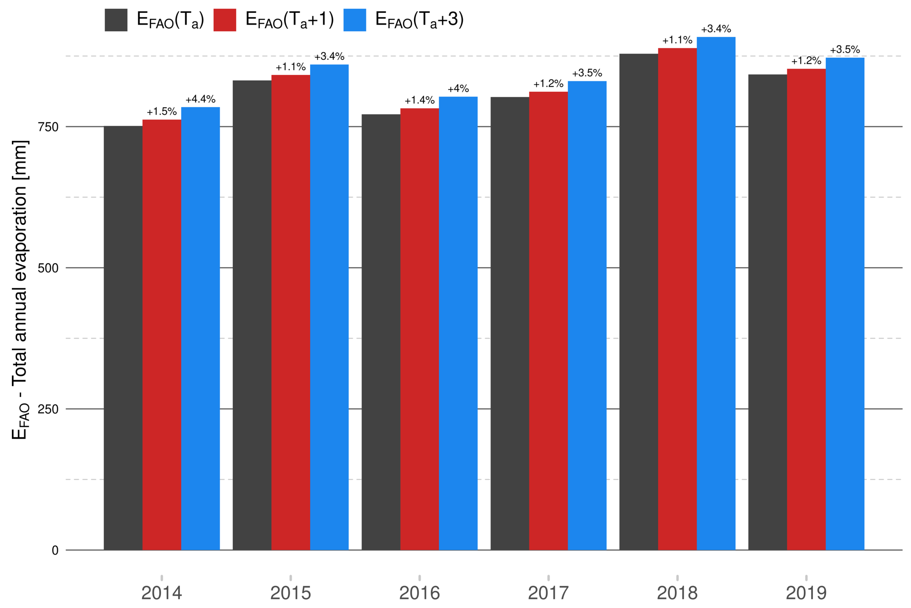
Each area has its specific conditions and they are different even within one area of interest. The main reason why it is important to have the exact measured climate data in a sufficiently long time-series is presented in Figure 2. This graph shows the percentage increase in annual total evaporation calculated by the Penman–Monteith Equation (1) in the theoretical situation where we simulate the average temperature increase by 1 degree and 3 degrees. These results demonstrate the importance of exact input climate data.

3. Results

In

Table 1. Evaporation in the years 2014–2019 computed using various models presented in this paper. For the computation, we used original values of constants in the equations. Please note the significant differences between models.

		${\mathit{E}}_{\mathbf{FAO}}$	${\mathit{E}}_{\mathbf{S}}$	${\mathit{E}}_{\mathbf{BV}}$	${\mathit{E}}_{\mathbf{HS}}$	${\mathit{E}}_{\mathbf{Sch}}$	${\mathit{E}}_{\mathbf{PT}}$	${\mathit{E}}_{\mathbf{K}}$	${\mathit{E}}_{\mathbf{VUV}}$
Year	2014	751	869	872	871	821	877	908	763
	2015	832	937	875	913	932	904	924	810
	2016	772	872	844	874	832	877	896	744
	2017	802	881	857	893	870	884	917	823
	2018	879	1022	916	967	1007	976	1020	826
	2019	842	958	904	894	951	934	967	832

, the summary of annual evaporation totals is given to illustrate how a wide range of computed results could be. For example, in the year 2018 one could expect evaporation between 826 mm (VUV equation) and 1022 mm (Šermer equation estimate); such a huge difference is crucial when planning the flooding of the former mine. In the case of Lake Most, with a surface area 309 ha, the difference of (nearly) 200 mm means (approximately) 600,000 m${}^3$ of water to be purchased.

We summarize the results of our calibration process in

Table 2. Comparison of original models and calibrated models. We denote the calibrated models with optimal parameters by $E^{*}=E\left({\theta }^{*}\right)$.

	Original Model	Calibrated Model
Šermer	$E_{\mathrm{S}}={10}^{0.0452T_a-0.204}$	$E_{\mathrm{S}}^{*}={10}^{0.03862T_a-0.1704}$
Beran–Vizina	$E_{\mathrm{BV}}=0.2157T_a+1.1133$	$E_{\mathrm{BV}}^{*}=0.239T_a-0.6103$
Hargreaves–Samani	$E_{\mathrm{HS}}\left(\theta \right)=\frac{0.0023R_a(T_a+17.8)\sqrt{T_r}}{\lambda }$	$E_{\mathrm{HS}}{\left(\theta \right)}^{*}=\frac{0.002201R_a(T_a+13.94)\sqrt{T_r}}{\lambda }$
Schendel	$E_{\mathrm{Sch}}=16\frac{T_a}{RH}$	$E_{\mathrm{Sch}}^{*}=13.58\frac{T_a}{RH}$
Priestley–Taylor	$E_{\mathrm{PT}}=\frac{1.26\Delta (R_n-G)}{\lambda (\Delta +\gamma )}$	$E_{\mathrm{PT}}^{*}=\frac{1.05\Delta (R_n-G)}{\lambda (\Delta +\gamma )}$
Kharrufa	$E_{\mathrm{K}}=0.34p{T}_a^{1.3}$	$E_{\mathrm{K}}^{*}=0.6392p{T}_a^{0.9922}$
VUV	$E_{\mathrm{VUV}}=0.2157T_a+0.726u_2-1.2259$	$E_{\mathrm{VUV}}^{*}=0.2404T_a+0.03841u_2-0.6853$

. Here we compare the models with original values proposed by authors and our new optimal values obtained through the solution of Equation (20). For obtaining these values, we used only the years 2014–2018. The rest of the time-series was used for validation.

The improvement of NSE values for original and calibrated models on both the training and validation parts of the data is presented in

Table 3. Comparison of the Nash–Sutcliffe efficiency (NSE) for the model with original constants and the calibrated models. The value closer to 1 is better.

	Training		Validation		All
	Original	Calibrated	Original	Calibrated	Original	Calibrated	%
Šermer	0.6157	0.7597	0.6440	0.7772	0.6210	0.7629	$+23\%$
Beran–Vizina	0.7326	0.7795	0.7342	0.7809	0.7330	0.7798	$+6\%$
Hargreaves–Samani	0.8819	0.9522	0.9157	0.9426	0.8881	0.9505	$+7\%$
Schendel	0.7621	0.8317	0.7902	0.8642	0.7673	0.8377	$+9\%$
Priestley–Taylor	0.9045	0.9989	0.9099	0.9990	0.9055	0.9989	$+10\%$
Kharrufa	0.6396	0.8632	0.6659	0.8618	0.6445	0.8630	$+34\%$
VUV	0.6284	0.7799	0.6561	0.7835	0.6336	0.7806	$+23\%$

. The improvement is compared also in the form of scatter plots and the graphs of cumulative values in Figure 3, Figure 4, Figure 5, Figure 6, Figure 7, Figure 8 and Figure 9, and in the form of annual total evaporation in Figure 10.

Finally, in

Table 4. Evaporation in the years 2014–2019 computed using the calibrated models presented in this paper.

		${\mathit{E}}_{\mathbf{FAO}}$	${\mathit{E}}_{\mathbf{S}}^{*}$	${\mathit{E}}_{\mathbf{BV}}^{*}$	${\mathit{E}}_{\mathbf{HS}}^{*}$	${\mathit{E}}_{\mathbf{Sch}}^{*}$	${\mathit{E}}_{\mathbf{PT}}^{*}$	${\mathit{E}}_{\mathbf{K}}^{*}$	${\mathit{E}}_{\mathbf{VUV}}^{*}$
Year	2014	751	751	727	732	697	731	744	726
	2015	832	792	726	767	791	753	748	727
	2016	772	749	703	735	706	731	728	703
	2017	802	755	720	751	739	736	744	722
	2018	879	851	790	818	854	813	800	790
	2019	842	809	809	754	807	778	778	761

we present the annual evaporation totals computed by the calibrated models and their comparison with $E_{FAO}$ results. It can be seen how the range of computed results was narrowed down when the equations with calibrated coefficients were used.

4. Discussion

The calibration process improved the NSE value of all models, see Table 3. The method minimizes the sum of squares of differences between model values and FAO values divided by a constant (see (20)) and, therefore, the differences were minimized and consequently the scatter plots are more clumped around the equality line; see Figure 3, Figure 4, Figure 5, Figure 6, Figure 7, Figure 8 and Figure 9. This property is typical for NSE, see [30]. The cumulative evaporation values show that all original models overestimated and all calibrated models underestimated the total evaporation.

This property can also be seen from the annual total evaporation, see Figure 10. For every year, we have computed the percentage of the difference between FAO values and model values, i.e., PBIAS, and plotted these values on the top of the bars in Figure 10. The differences in average PBIAS values for the original and calibrated models are presented in

Table 5. Comparison of average PBIAS for annual total evaporation between original and calibrated models, see Figure 10. For the comparison, we also included the percentage of NSE improvement from Table 3. In our calibration process, we focused only on NSE values and therefore, the value of PBIAS can be worse.

	${\mathit{E}}_{\mathbf{S}}^{*}$	${\mathit{E}}_{\mathbf{BV}}^{*}$	${\mathit{E}}_{\mathbf{HS}}^{*}$	${\mathit{E}}_{\mathbf{Sch}}^{*}$	${\mathit{E}}_{\mathbf{PT}}^{*}$	${\mathit{E}}_{\mathbf{K}}^{*}$	${\mathit{E}}_{\mathbf{VUV}}^{*}$
PBIAS original	$13.5\%$	$8\%$	$10.9\%$	$10.9\%$	$11.8\%$	$15.5\%$	$-1.7\%$
PBIAS calibrated	$-3.4\%$	$-9.1\%$	$-6.4\%$	$-5.9\%$	$-6.8\%$	$-6.8\%$	$-9.1\%$
NSE improvement	$23\%$	$6\%$	$7\%$	$9\%$	$10\%$	$34\%$	$23\%$

.

5. Conclusions

In this paper, we examined and discussed the calibration of selected evaporation models against the Penman–Monteith equation in terms of the Nash–Sutcliffe efficiency maximization.

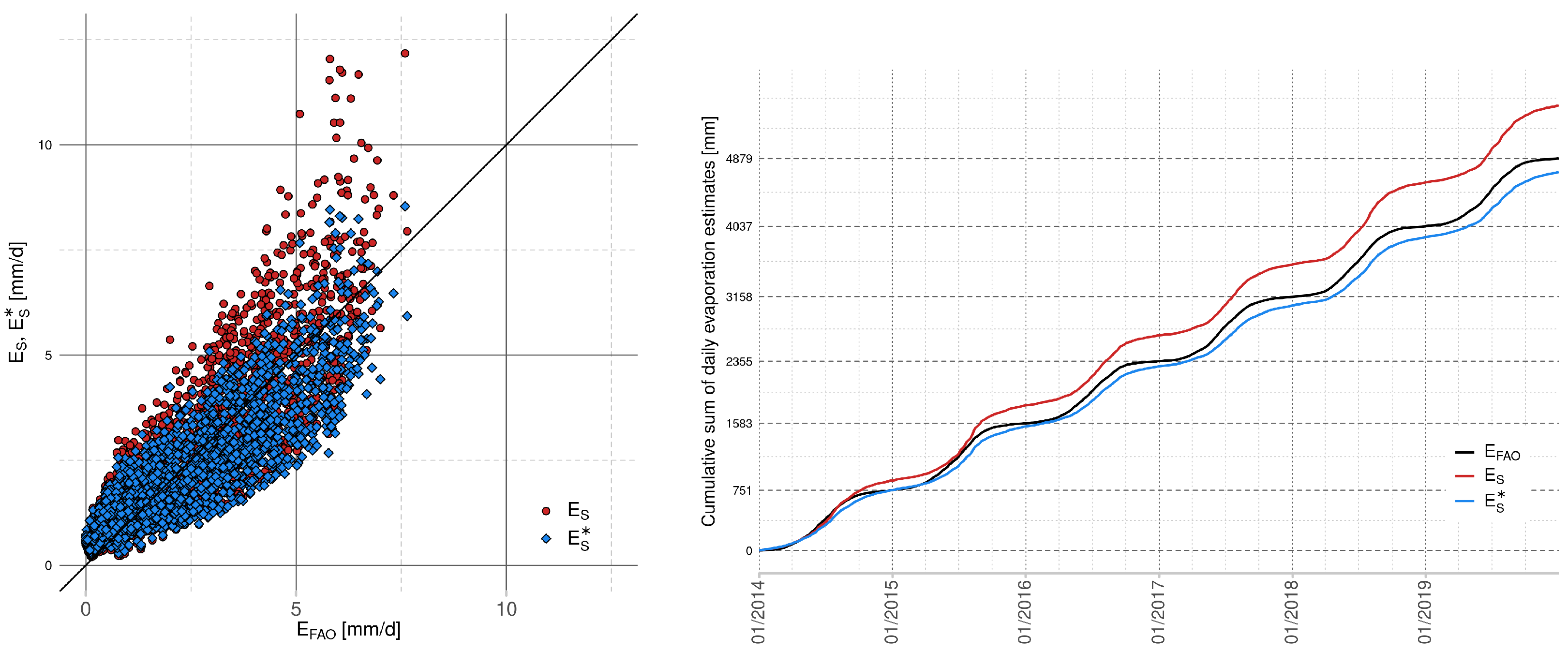
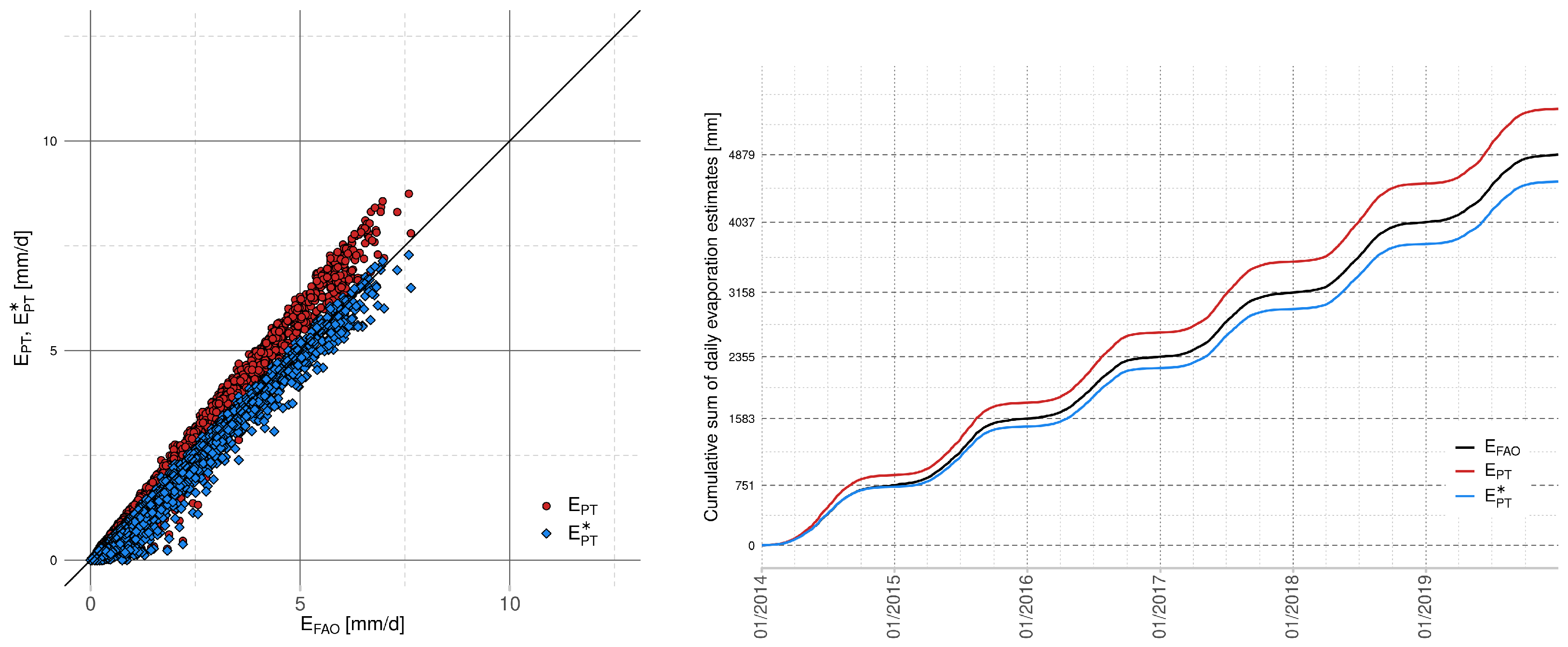
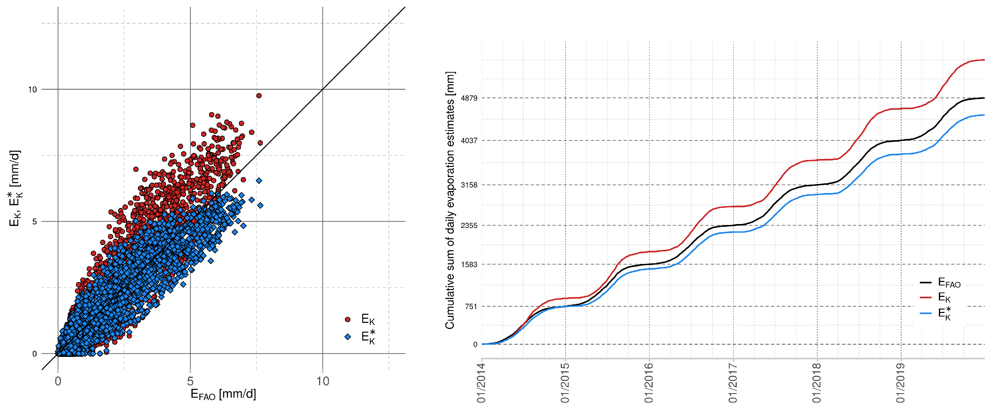
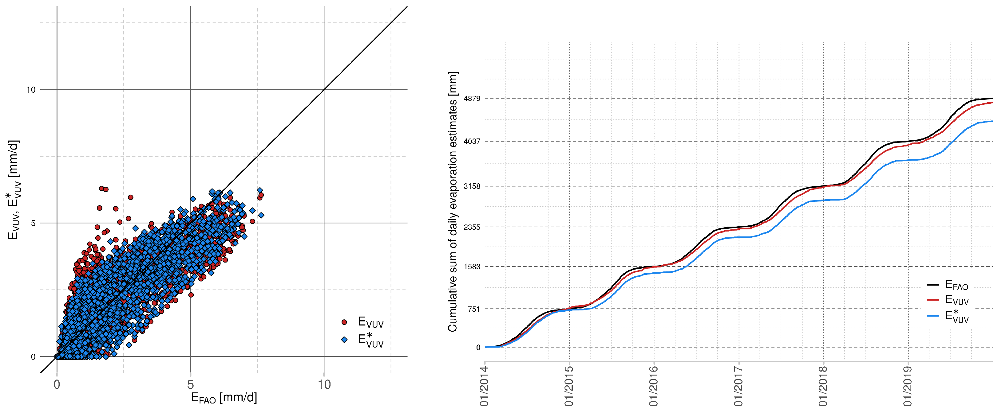
From our results, found using data from our area of interest (Lake Most), we suggest approximating the Penman–Monteith equation by using the calibrated Hagreaves–Samani equation. This choice is supported by the presented comparison of scatter plots of evaporation values and cumulative evaporation graphs. The calibration improves the value of optimized fitting criteria; however, the choice of the optimal simplified model depends not only on the ability to approximate the evaporation values in terms of the selected statistical measure but also on the input measurement requirements. In the case of the suggested Hagreaves–Samani equation, one has to provide measurements of air temperature and extraterrestrial radiation, which is computed from the latitude of the considered area and the serial number of the day of the year.

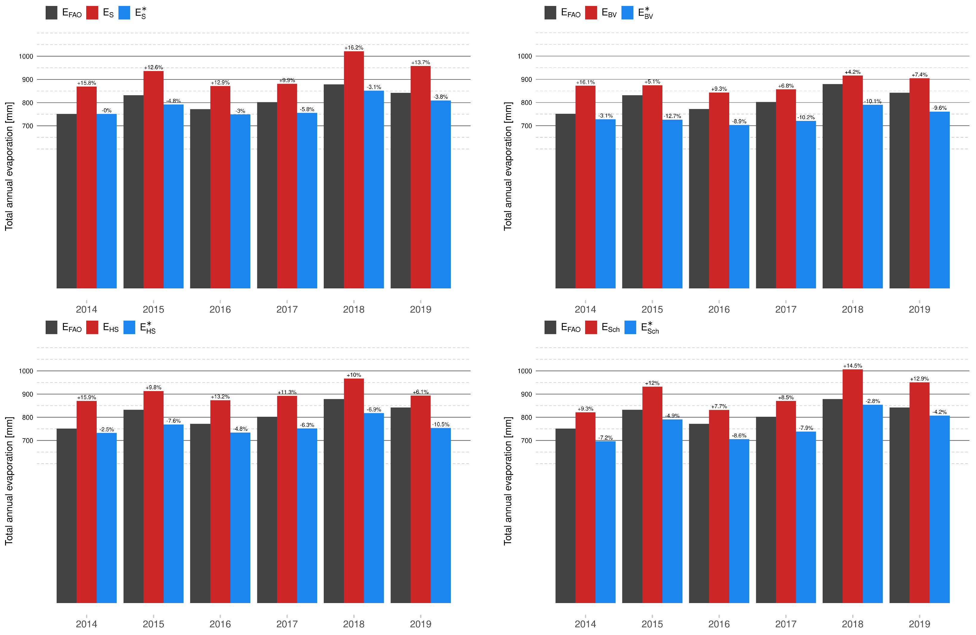
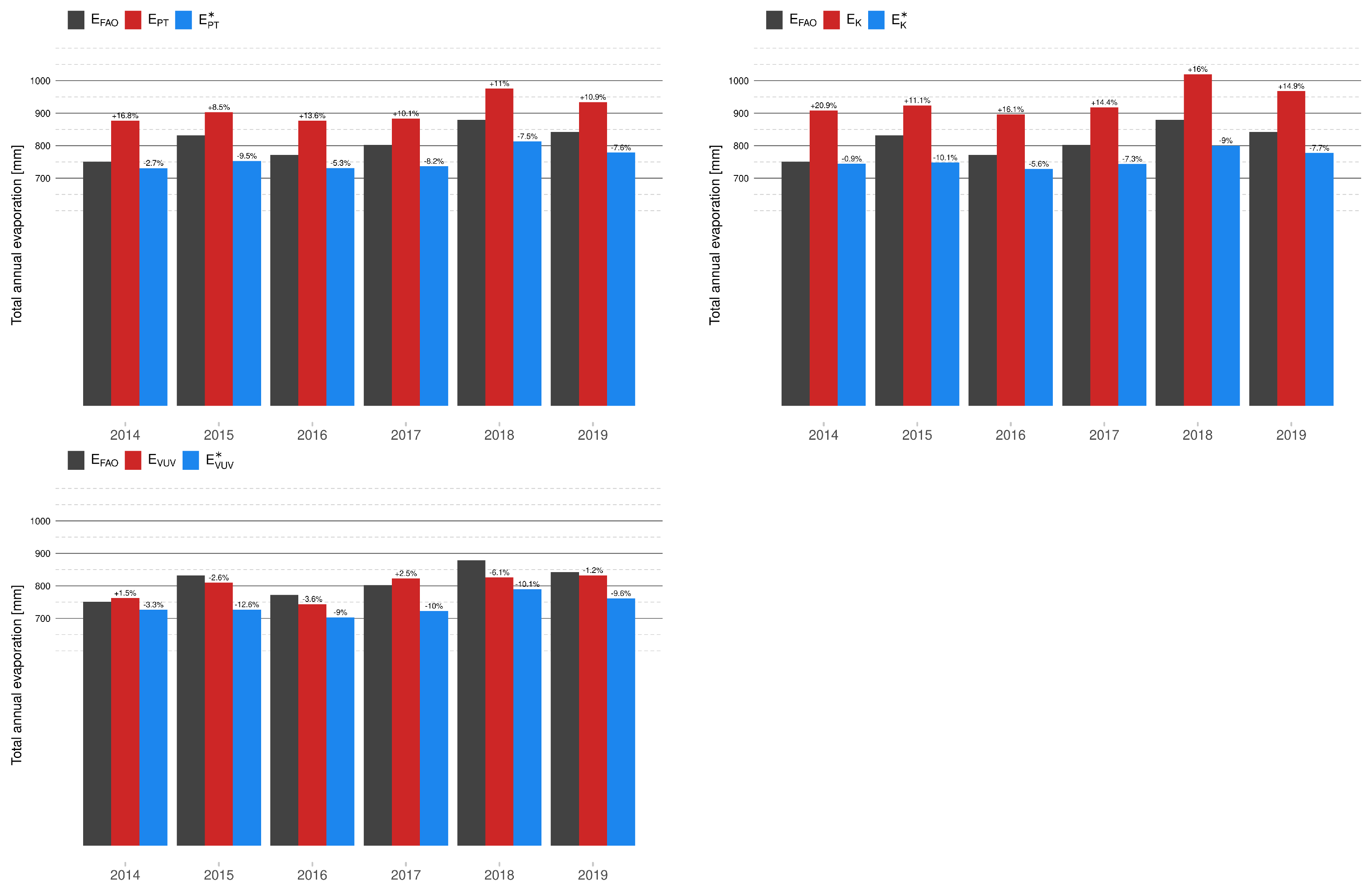
Additionally, we observed that the calibration based on the Nash–Sutcliffe efficiency can simultaneously degrade the value of other statistical measures, namely percentage bias. This value is directly connected with the estimation of annual total evaporation. From all considered models in this paper, the calibrated Hagreaves–Samani equation is not only able to approximate the evaporation in terms of optimal Nash-Sutcliffe efficiency, but the decrease of percentage bias is also small, as well as the demand on input data. However, the final decision is dedicated to the securer of the area.

In this paper, we examined the calibration of seven models of different types; however, our methodology can be easily applied to any state-of-the-art method.

In our ongoing research, we will extend our comparison through the consideration of other stochastic measures to examine how the choice of objective measures in the calibration process influences the properties of calibrated models. Additionally, we will focus on the examination of the presented calibration process and calibrated models using real-world measurements of evaporation on Lake Most.