Poverty and Physical Geographic Factors: An Empirical Analysis of Sichuan Province Using the GWR Model

Abstract

Given the complexity of the poverty problem, efforts and policies aiming at reducing poverty should be tailored to local conditions, including cultural, economic, social, and geographic aspects. Taking the Sichuan Province of China as the study area, this paper explores the impact of physical geographic factors on poverty using the Ordinary Least Squares (OLS) Regression and the Geographically Weighted Regression (GWR) models at the county level. In total, 28 factors classified in seven groups were considered as variables, including terrain (relief degree of the land surface, altitude, and slope); vegetation (forest coverage rate); water (drainage network density); climate (temperature, annual average rainfall); and natural disaster (landslide, debris flow, and torrential flood). The 28 variables were then tested using correlations and regressions. A total of six physical variables remained significant for the OLS and GWR models. The results showed that the local GWR model was superior to the OLS regression model and, hence, more suitable for explaining the associations between the poverty rate and physical geographic features in Sichuan.

1. Introduction

China has been waging a national war against poverty for the past several decades. Remarkable progress has been achieved for the country as a whole and in particular as the poverty rate in China dropped dramatically from 10.2% to 3.1% from 2012 to 2017 [1]. Despite this remarkable achievement, China still faces the poverty issue. It is still an essential obstacle to the sustainable development of Sichuan Province and the equity issue for Sichuanese people. Poverty reduction is always one of the core issues of regional sustainable development. Globally, the root causes of poverty and effective ways to reduce poverty are high-priority research and policy concerns. Scholars and policymakers often hold different perspectives. Among them, the relationship between poverty and geographic factors has been shown to be intriguingly significant [2]. Furthermore, our own numerous field trips in Sichuan Province, where agriculture is dominant, also reveal that the quality of life for the area’s farmers does vary over diverse terrains and climate conditions. However, fundamental questions on whether this effect exists, how significant the effect is, and what the main spatial patterns are for major geographic factors call for formal investigations.

In this study, we consider a total of 28 physical geographic variables, including the relief degree of land surface (RDLS), forest coverage rate, drainage network density, temperature, rainfall, torrential flood danger, debris flow danger, landslide danger, altitude, and slope. We conduct a thorough study with the most extensive collection of physical geographic variables, hoping to meaningfully contribute to the existing knowledge of poverty in Sichuan Province. Furthermore, we answer the two following specific research questions: What are the physical geographic factors having a significant impact on poverty? Can spatial analysis based on the GWR help poverty reduction?

Specifically, we demonstrate variables’ selection, model formulation, and analysis of factors at the county scale.

2. Literature Review

The literature shows that the relationship between man and the environment was recognized a long time ago. As early as the Montesquieu era, the relationship between climate and human characteristics was documented [3]. Semple conducted a systematic study on the influence of geographical elements [4]. Huntington believed that civilization’s distribution was consistent with the distribution of climate-based health and energy [5]. Poverty as a comprehensive development problem was directly linked to the geographical environment in the 1960s when Thompson proposed the geography of poverty [6]. Later, more theories and case studies on poverty were published in the U.S. [7,8], Ireland [9,10], and Scotland [11,12]. The concept of spatial poverty traps has made the geographic dimension of poverty more attractive to scholars from various disciplines. At the end of the 1990s, World Bank experts verified the spatial poverty trap’s existence through the empirical analysis of the farm household panel data over the period 1985–1990 for rural areas in southern China [13,14]. Thomas and his partners found that geospatial divergence and human capital might be good explanatory predictors for regional poverty traps [15]. David confirmed the existence of spatial poverty traps by many empirical analyses [16]. Paraguas and Kamil analyzed the spatial dimensions of poverty and its determinants by using a spatial econometrics model in Bangladesh [17]. Ebizimor and Dare analyzed the socio-spatial dynamics of poverty in the three Senatorial Districts of Delta State, Nigeria, to figure out the impact of geospatial factors on the poverty changes over space [18].

In China, the Chinese government has been fighting poverty in concerted efforts recently. Chinese scholars have conducted extensive research on the spatial pattern of poverty and the relation between poverty and geospatial factors using various quantitative methods, including correlation analysis [19], spatial analysis in GIS (geographic information system) [20], or a combination of the two [21], geostatistical methods [22], and geo-detectors [23]. A regional poverty framework was also constructed from the perspective of geography [24]. Liu et al. analyzed rural poverty for the entirety of China and found that the Chinese rural poor showed a clear spatial agglomeration pattern [25]. Niu et al. developed a Multi-source Data Poverty Index using social media data and remote sensing images to study city poverty in Guangzhou [26]. These studies substantially advanced poverty research and sustainable development at the regional and national levels in China.

The literature shows that the regression analysis technique is one of the most common methods used for uncovering the relations between poverty and geospatial factors, especially regarding the relative importance of possible factors [27], including socio-economic [28,29], physical geographic [30], demographic and health [31], and natural disasters [32]. However, it should be clear that in spatial poverty studies, especially at the regional or national scale, i.e., the entire Sichuan province or China, regression models could cause the so-called spatially non-stationary issue. This usually means that regression coefficients are not fixed spatially while they should be [33,34]. Therefore, in the literature, the Geographically Weighted Regression (GWR) [35] model was quite commonly used to identify the relationships between poverty and the factors over space and to map the spatial pattern of the coefficients [36].

Todd et al. applied the GWR model to analyze rural Malawi and found that there was strong evidence of the spatial divergence of the relationship between poverty and its determinants [37]. Xu et al. provided a theoretical framework to demonstrate the linkage of the geographic factors and regional poverty and used the GWR model to analyze this linage quantitatively [37]. Moreover, some studies used the GWR model to analyze the relationship between poverty and vegetation spatial distribution in the U.S. [38]. One research in Guizhou, China, showed that the GWR model could identify well that the slope and the distance to the local urban center were key determinants of spatial variations in rural poverty at the county level [39]. Similar studies in Malaysia showed clearly that road density and non-primary agricultural areas’ percentage are significant to poverty in the GWR model [40]. Guo et al. also applied the GWR model in urban poverty research and found that the significant factors in Western cities are also mostly relevant in Hong Kong [41]. Similar studies using the GWR model can be found on fuel poverty in England [42] and travel poverty in north-west England [43].

The representative pieces reviewed above provide concepts and models for poverty research and reduction policymaking. For a vast country such as China, its own geographical conditions vary widely and the factors contributing to poverty are vast as well. The same is true for a large province such as Sichuan. Therefore, we limit our research focus on geographic variables and investigate their impacts on poverty in Sichuan, with an expectation to find something universal for similar inquires beyond Sichuan.

3. Study Area

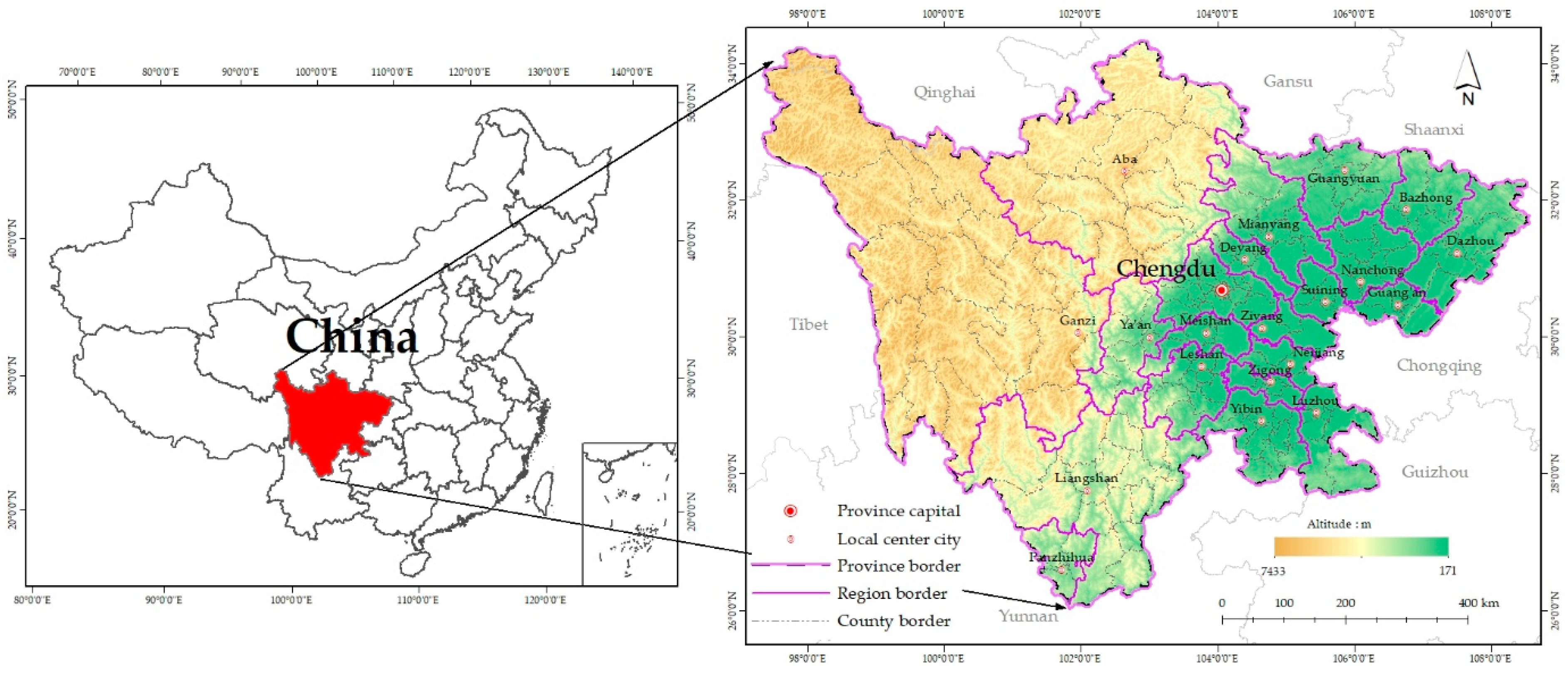
Sichuan province is located in the southwest of China. It is also in the upstream area of the Yangtze River drainage basin. It is within the extent of 92°21′ to 108°12′ E and 26°03′ to 34°19′ N. It is 1075 km from east to west and more than 900 km from north to south. Its east is adjacent to Chongqing city. Yunnan and Guizhou provinces are adjacent to its south. Moreover, the western neighbor is Tibet. The three provinces of Shaanxi, Gansu, and Qinghai are its northern neighbors (Figure 1). The province covers an area of 486,000 km², including 183 county-level administrative units. It is particularly obvious that the terrain is high in the west and low in the east. The western part is mountainous areas with an altitude of more than 4000 m. The eastern part is basin and hills with an altitude from 1000 to 3000 m. The entire province can be divided into three parts: Sichuan Basin, Northwestern Sichuan Plateau, and Southwestern Sichuan Mountain [44].

Figure 1. The location map of Sichuan province.

At the end of 2018, the GDP of Sichuan Province was USD 0.592976 trillion (exchange rate on 31 December 2018), and the per capita GDP was USD 7125.80 [45]. At the same time, the number of permanent residents living in Sichuan was 83.41 million. Among them, the urban population was 43.615 million, and the urbanization rate was 52.29% [46]. However, the spatial distribution of population density is very uneven. The regions with the highest population density are concentrated in the seven municipalities in the east, and the regions with the lowest population density are concentrated in the Aba and Ganzi regions in the west. At the end of 2016, there were a total of 2.17 million poor people in Sichuan Province [47]. Among them, 739,000 poor people lived in the poverty-stricken counties [48]. They were mainly distributed in ethnic-minority areas with complex geographical conditions, including harsh and fragile physical conditions.

4. Data

In this study, DEM (digital elevation model), climate data, drainage network, land use, geological disaster, and administrative data were used in the analysis. DEM was acquired from the USGS (the United States Geological Survey) website. Climate data, including temperature and rainfall, drainage network, land use, and administrator data, were provided by the Data Center for Resources and Environmental Sciences, Chinese Academy of Sciences (RESDC, CAS). Geological disaster data came from the Institute of Mountain Hazards and Environment, Chinese Academy of Sciences and Ministry of Water Conservancy. We obtained poverty data from province and county government work reports in 2015.

All the data were entered into GIS geodatabase after preprocessing. Furthermore, the projection and coordinate system of all the data were transformed into UTM84N, WGS-84, in GIS software.

4.1. Variables Selection

The poverty rate was the dependent variable (Y). The 28 physical geographic variables included six climate variables: temperature rate 1 (T1), temperature rate 2 (T2), temperature rate 3 (T3), temperature rate 4 (T4), temperature rate 5 (T5) [49], and annual average rainfall (R); 11 terrain variables: altitude rate 1 (A1), altitude rate 2 (A2), altitude rate 3 (A3), altitude rate 4 (A4), altitude rate 5 (A5), slope rate 1 (S1), slope rate 2 (S2), slope rate 3 (S3), slope rate 4 (S4), slope rate 5 (S5) [50], and relief degree of the land surface (RDLS) [14,51]; 9 geological disaster variables: torrential flood with high-danger rate (TFH), torrential flood with medium-danger rate (TFM), torrential flood low-danger rate (TFL), landslide with high-danger rate (LSH), landslide with medium-danger rate (LSM), landslide with low-danger rate (LSL), debris flow with high-danger rate (DFH), debris flow with medium-danger rate (DFM), and debris flow with low-danger rate (DFL); and 2 physical resource variables: forest coverage rate (FR) and drainage network density (DND) [50]. The description of each variable is shown in Table 1.

Table 1. Description of variables and measures.

Group	Variables	Description	Calculation	Units
Climate	T1	Rate of days with max temp ≥ 28 °C	Days with max temperature ≥ 28 °C/365	%
	T2	Rate of days with 10 °C < max temp < 28 °C	Days with 10 °C < max temperature < 28 °C/365	%
	T3	Rate of days with max temperature ≤ 10 °C	Days with max temperature ≤ 10 °C/365	%
	T4	Rate of days with 10 °C < min temp ≤ 28 °C	Days with 10 °C < min temperature ≤ 28 °C/365	%
	T5	Rate of days with min temp ≤ 10 °C	Days with min temperature ≤ 10 °C/365	%
	R	annual average rainfall	get directly	mm
Terrain	A1	Rate of area with altitude 0 to 800 m	Area with altitude from 0 to 800 m/county area	%
	A2	Rate of area with altitude 800 to 1800 m	Area with altitude from 800–1800 m/county area	%
	A3	Rate of area with altitude 1800 to 2800 m	Area with altitude from 1800–2800 m/county area	%
	A4	Rate of area with altitude 2800 to 3600 m	Area with altitude from 2800–3600 m/county area	%
	A5	Rate of area with altitude above 3600 m	Area with altitude above 3600 m/county area	%
	S1	Rate of area with slope of 0–2°	Area with slope of 0–2°/county area	%
	S2	Rate of area with slope of 2–5°	Area with slope of 2–5°/county area	%
	S3	Rate of area with slope of 5–15°	Area with slope of 5–15°/county area	%
	S4	Rate of area with slope of 15–25°	Area with slope of 15–25°/county area	%
	S5	Rate of area with slope above 25°	Area with slope above 25°/county area	%
	RDLS	Relief degree of the land surface	Method comes from Feng [51]
Geological disasters	TFH	Area rate of torrential flood high-danger	Area of torrential flood high-danger/county area	%
	TFM	Area rate of torrential flood medium-danger	Area of torrential flood medium-danger/county area	%
	TFL	Area rate of torrential flood low-danger	Area of torrential flood low-danger/county area	%
	LSH	Area rate of landslide high-danger	Area of landslide high-danger/county area	%
	LSM	Area rate of landslide medium-danger	Area of landslide medium-danger/county area	%
	LSL	Area rate of landslide low-danger	Area of landslide low-danger/county area	%
	DFH	Area rate of debris flow high-danger	Area of debris flow high-danger/county area	%
	DFM	Area rate of debris flow medium-danger	Area of debris flow medium-danger/county area	%
	DFL	Area rate of debris flow low-danger	Area of debris flow low-danger/county area	%
Physical resources	FR	Forest coverage rate	Forest area/county area	%
	DND	Drainage network density	Total length of drainage network/county area	km/km2
	Y	Poverty rate	Poor population/county population	%

4.2. Variables Characteristics

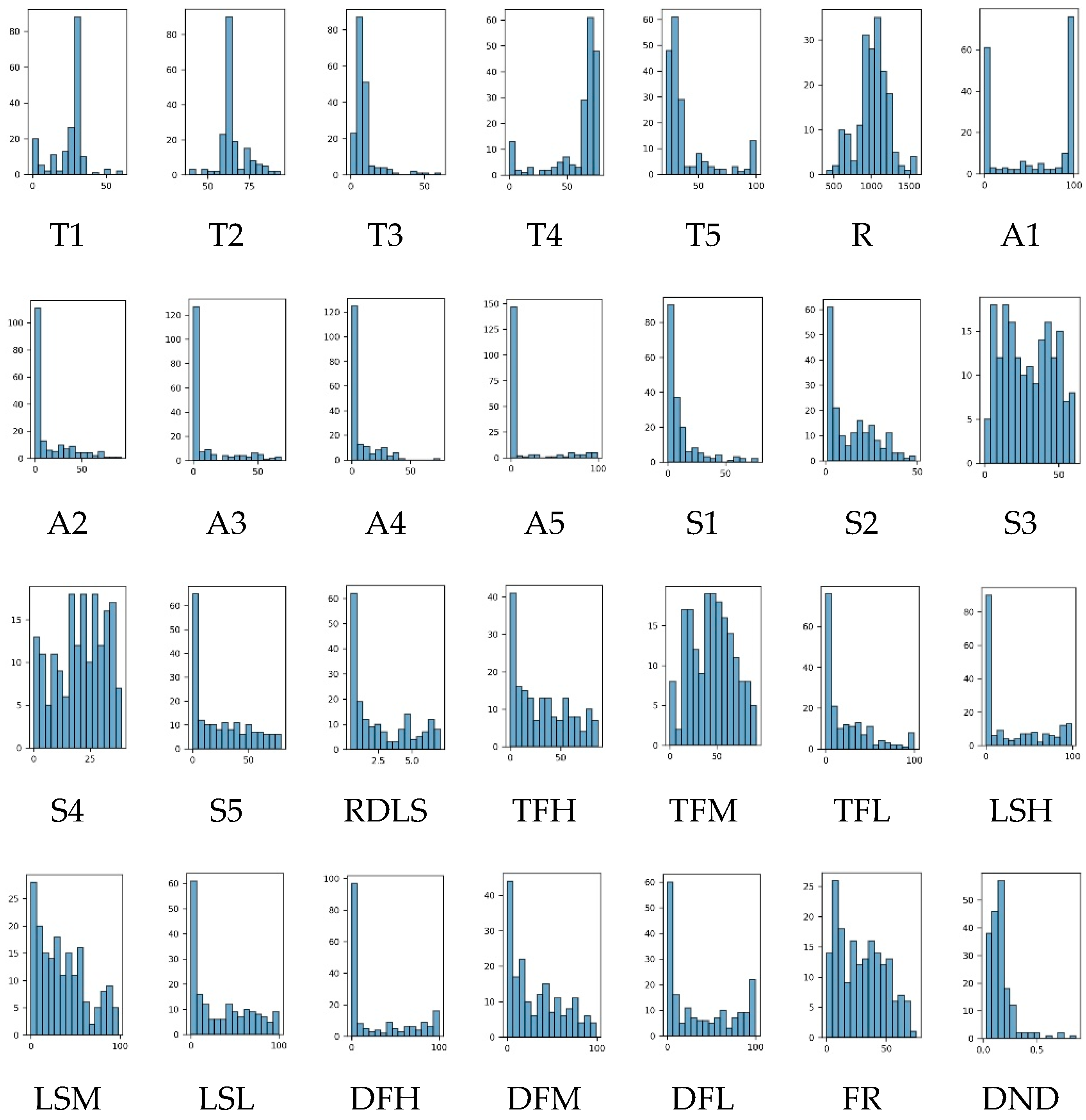
We first performed a descriptive statistical analysis of the selected variables, and the results are shown in Table 2. The minimum value of the poverty rate was 0.00%, while the poverty rate’s maximum value was 30.33%. The mean value of the poverty rate was 7.47%. There were 183 districts and counties in the province that participated in the statistical analysis. We used the Python package to make histograms for all the variables to their distributions. Except for the histograms of the variables R and TFM which were close to the normal distribution, the other variables’ histograms were skewed, as shown in Figure 2. Usually, skewed variables are better transformed with logarithm or similar before running Ordinary Least Squares (OLS). However, our preliminary OLS analyses indicated that even with some or all logarithmic transformations of dependent and independent variables, the results were not much different from those without transformations. Furthermore, considering spatial heterogeneity of the climate, terrain, geological and physical resources, and spatial autocorrelation of poverty rates, we believe the direct use of the variables in OLS, together with Moran’s I test, is reasonable to select significant variables, which can be further enhanced by Geographically Weighted Regression. The specifics of the methods are discussed in Section 5 in the Methods.

Table 2. Statistics characteristic of dependent and independent variables.

Variables		Min	Max	Mean	SD	Observations
Dependent variable Y		0	30.3	7.47	6.23	183
Independent variable	T1	0	61	25.32	11.45	183
	T2	39	94	65.1	8.66	183
	T3	0	61	9.59	8.23	183
	T4	0	78	60.7	21.08	183
	T5	22	100	39.3	21.08	183
	R	409	1599	1019.5	206.26	183
	A1	0	100	55.34	44.35	183
	A2	0	92	14.36	21.73	183
	A3	0	68	9.77	17.87	183
	A4	0	75	6.63	11.84	183
	A5	0	99	12.64	27.85	183
	S1	0	78	10.7	15.38	183
	S2	1	49	14.22	12.32	183
	S3	0	61	29.38	16.53	183
	S4	0	39	20.67	10.89	183
	S5	0	79	24.98	24.11	183
	RDLS	0.5	7.08	2.65	2.14	183
	TFH	0	87	32.31	26.29	183
	TFM	0	92	44.78	22.55	183
	TFL	0	100	22.84	26.67	183
	LSH	0	99	30.07	35.29	183
	LSM	0	98	36.62	27.14	183
	LSL	0	100	33.3	32.15	183
	DFH	0	100	28.56	36.31	183
	DFM	0	99	33.27	28.76	183
	DFL	0	100	38.12	36.63	183
	FR	0	75	29.09	19.24	183
	DND	0	0.87	0.16	0.12	183

Figure 2. Histogram distribution of variables.

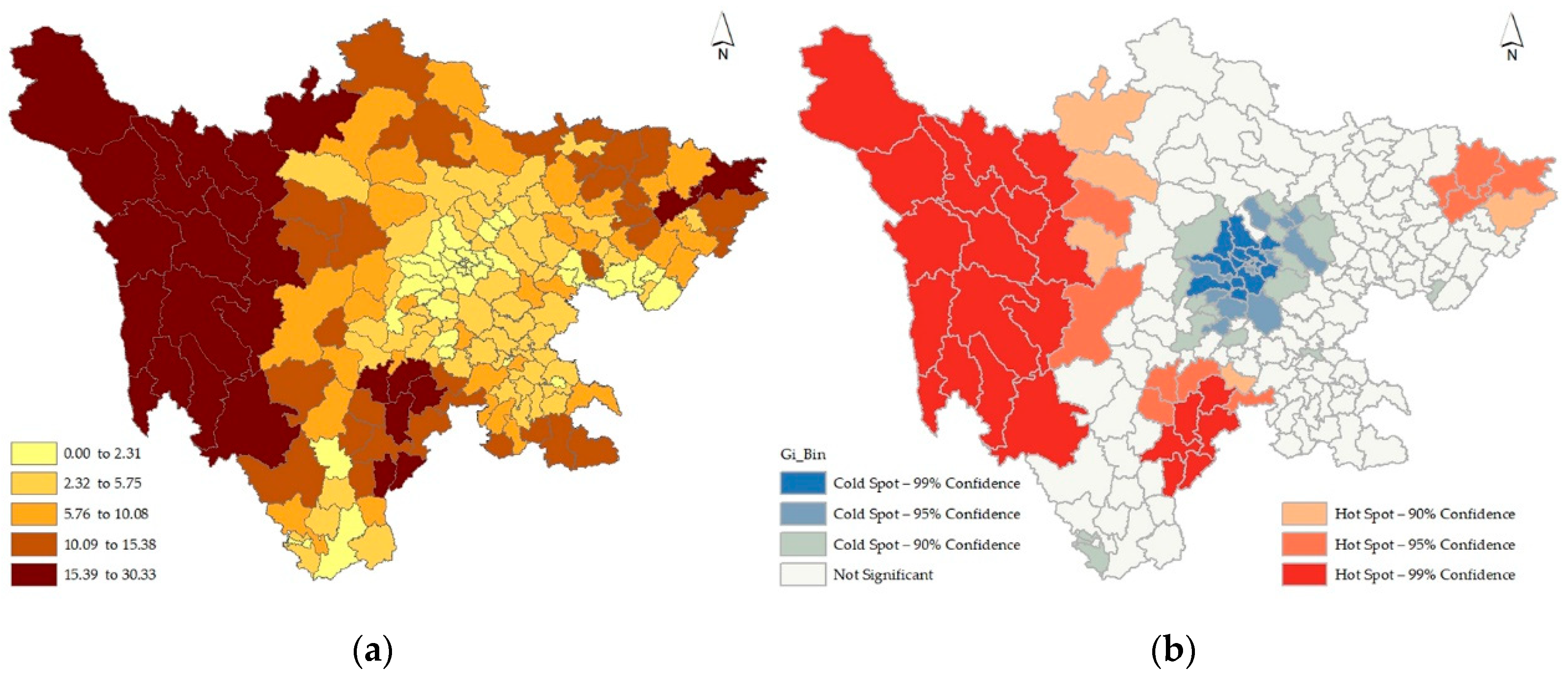
The spatial patterns of the poverty distribution at the county level are displayed in Figure 3. We found that high poverty rates are clustered in the western, southern, and northeastern parts of Sichuan. Jinyang County of Liangshan Yi Autonomous Prefecture had the highest poverty rate at 30.33%. To further illustrate the spatial distribution pattern of poverty rates, we performed a hot spot analysis for the province, and it was clear that the poverty clustered spatially significantly in Sichuan.

Figure 3. The spatial pattern of poverty in Sichuan province: (a) poverty rate distribution over the province; (b) hot spot analysis of poverty rate in Sichuan.

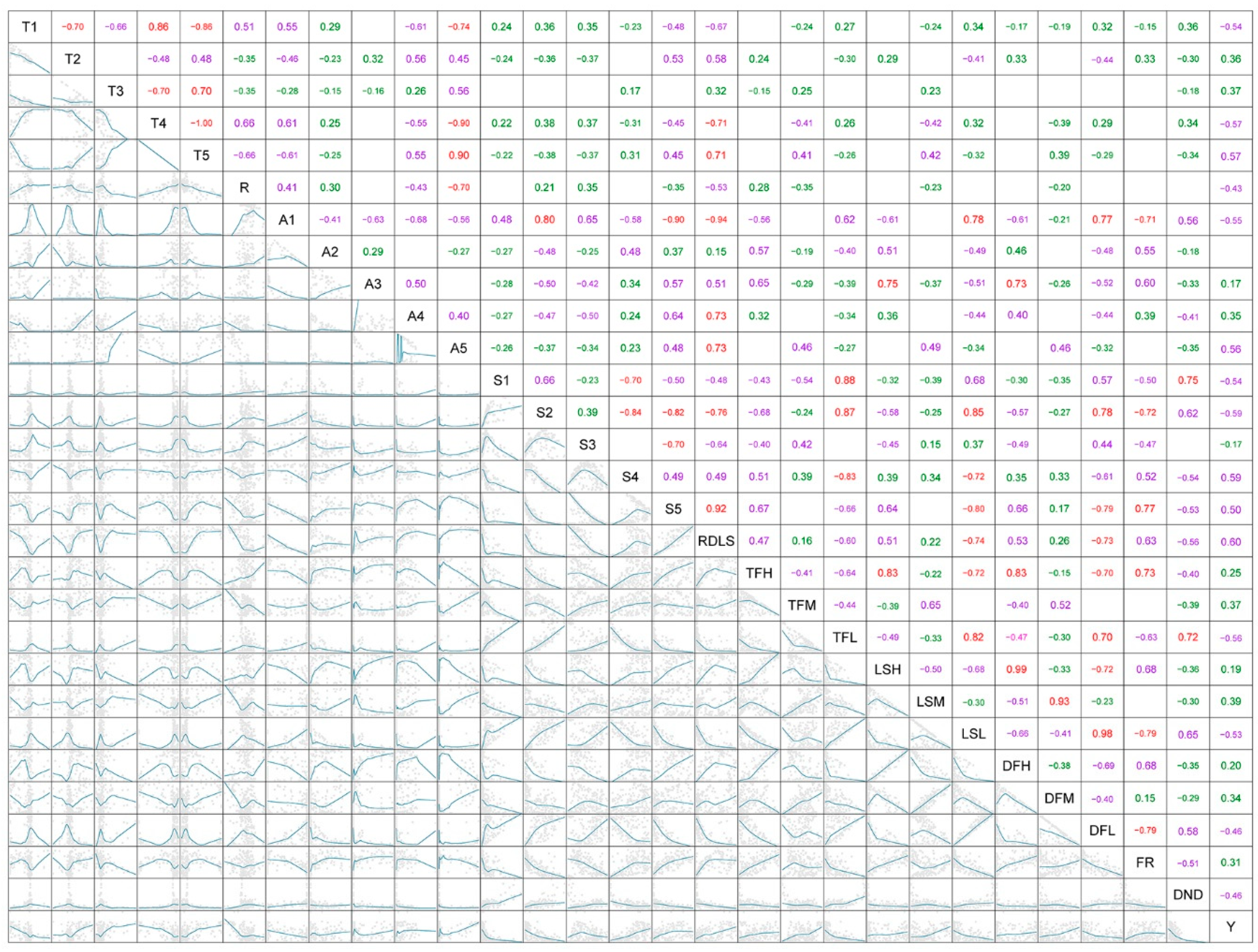
The Pearson correlation analysis of variables affecting poverty in all districts and counties in Sichuan province using R language [52] is illustrated in Figure 4. Variables, by groups, are shown on the diagonal. Bivariate scatter plots with fitted lines are displayed on the lower left corner of the diagonal, and the correlation coefficients are on the upper right corner of the diagonal. Their correlations were significant at the 0.05 level. Generally, if two variables’ correlation coefficient is equal to or above 0.7 (equal to or less than −0.7), we can say that the two variables have a strong correlation. If the correlation coefficient is equal to or above 0.4 and less than 0.7 (above −0.7 and equal to or less than −0.4), the two variables have a moderate correlation. Moreover, if the correlation coefficient is less than 0.4 (above −0.4), they have a weak correlation; and if the correlation coefficient is equal to 0, the two variables have no correlation [52]. In Figure 4, the colors of the numbers indicate the correlation strength between the variables—the red color indicates a strong correlation, the purple color indicates a moderate correlation, and the green color indicates a weak correlation.

Figure 4. The correlations and scatter plot matrices for all variable pairs.

More specifically, we could see that the fourth row and fifth column show that T4 and T5 had a perfect linear correlation. The correlation coefficient of the two variables was −1, with a p-value of less than 0.0001. In addition, the correlation coefficients of T1 and T2, T1 and T4, T1 and T5, T3 and T4, T3 and T5, T4 and A5, T4 and RDLS, T5 and A5, T5 and RDLS, A1 and S2, A1 and S5, A1 and RDLS, A1 and LSL, A1 and DFL, A1 and FR, A3 and LSH, A3 and DFH, A4 and RDLS, A5 and RDLS, S1 and S4, S1 and TFL, S1 and DND, S2 and S4, S2 and S5, S2 and RDLS, S2 and TFL, S2 and LSL, S2 and DFL, S2 and FR, S3 and S5, S4 and TFL, S4 and LSL, S5 and RDLS, S5 and LSL, S5 and DFL, S5 and FR, RDLS and LSL, RDLS and DFL, TFH and LSH, TFH and LSL, TFH and DFH, TFH and DFL, TFH and FR, TFL and LSL, TFL and DFL, TFL and DND, LSH and DFH, LSH and DFL, LSM and DFM, LSL and DFL, LSL and FR, and DFL and FR were equal to or above 0.7 or equal to or less than −0.7. They indicated strong correlation between these variables. For example, LSH-DFH = 0.99, LSL-DFL = 0.98, and LSM-DFM = 0.93, indicating high correlations between landslide and debris flow; S5-RDLS = 0.92, showing high correspondence between land slope and relief degree; and T5-A5 = 0.90, reflecting the lower temperature areas located at high altitude. Some strong negative correlations include T4-T5 = −1.0, indicating that temperature variations in colder areas are lower; A1-RDLS = −0.94, signifying that low slope were not in relief areas; and T4-A5 = −0.90, showing that areas at high altitude often face smaller temperature gaps for a typical day. For the poverty rate, with respect to each physical variable, the correlations range from Y-A2 = 0.07 to Y-RDLS = 0.60, specifying milder slopes for less poverty and high relief for higher poverty. All these make sense and correspond to historical records.

In the subsequent analysis of the OLS regression, if all factors with strong correlations were adopted in the model, it would cause the multicollinearity problem, which would make the model results unreliable. Therefore, before establishing the OLS regression model, we examined the 28 physical variables and eliminated multicollinearity.

5. Methods

5.1. Ordinary Least Squares Regression

In Section 4.2, we noticed that some factors have strong correlations. Therefore, prior to the GWR model regression analysis, the significance of the variables’ coefficients and the possible existence of multicollinearity problems [53] needed to be tested and identified to eliminate multicollinearity. Some methods exist to handle multicollinearity. They are stepwise regression, ridge regression, and principal component regression [54]. In this study, the stepwise regression method was used to deal with the multicollinearity problem in SPSS 22 [55]. Using stepwise regression, we found that temperature rate 2 (T2), temperature rate 3 (T3), annual average rainfall (R), altitude rate 4 (A4), slope rate 1 (S1), and slope rate 4 (S4) had reasonable VIFs (variable inflation factor), which were lower than 7.5. Furthermore, they were significant for the regression too. In this paper, the OLS regression model was used in GIS to examine the relationship between the independent variable (poverty rate) and the selected dependent variables at county level over the province. The OLS model was as below as:

$$PO={\beta }_0+{\beta }_1\mathrm{T}2+{\beta }_2\mathrm{T}3+{\beta }_3\mathrm{R}+{\beta }_4\mathrm{A}4+{\beta }_5\mathrm{S}1+{\beta }_6\mathrm{S}4+\epsilon$$

where dependent variable PO = poverty rate; ${\beta }_0$ = regression constant; ${\beta }_1 \mathrm{to} {\beta }_6$ = coefficients of independent physical geographic variables; and $\epsilon$ is the random error for the model.

Before running the OLS model, a spatial autocorrelation test for the poverty rate was performed to get its Moran’s I, which is defined as:

$$I=\frac{n}{{\displaystyle {\displaystyle \sum }_{i=1}^n}{\displaystyle {\displaystyle \sum }_{j=1}^n}{W}_{ij}}\times \frac{{\displaystyle {\displaystyle \sum }_{i=1}^n}{\displaystyle {\displaystyle \sum }_{j=1}^n}{W}_{ij}\left(x_i-\overline{x}\right)\left(x_j-\overline{x}\right)}{{\displaystyle {\displaystyle \sum }_{i=1}^n}{\left(x_i-\overline{x}\right)}^2}$$

where $n$ is the total number of counties in the province; $i$ and $j$ stand for different counties; $x_i$ is the residual of $i$; $\overline{x}$ is the mean of residuals; and $W_{ij}$ is a measure of spatial proximity pairs of $i$ and $j$. The values of Moran’s I are between −1 and 1 [56,57]. Negative autocorrelation values mean adjacent locations tend to be dispersed. Conversely, positive autocorrelation values indicate that the adjacent locations are similar. Moran’s I values are used with their z-scores and p-values for their significance to reject or accept the null hypothesis that a variable in a study area is or is not randomly distributed [58]. The Moran’s I value for poverty rate was 0.694089 and the z-score was 15.186465, which was much larger than the critical value of 2.58 for 99% confidence. Therefore, we could determine that the poverty rate had a spatial aggregation phenomenon with similar values, and the independent variables showed spatial heterogeneity. It was feasible to take the multivariate analysis of poverty through the OLS model. The results are shown in Table 3. We need to focus on the values of R², adjusted R², and AICc (Akaike’s Information Criterion) in this table.

Table 3. Results of Ordinary Least Squares (OLS) and spatial dependence tests.

Variable	Coefficient	StdError	p-Value	VIF
Intercept	0.307	4.045	0.93948	—
T2	0.174	0.044	0.00015	1.72
T3	0.179	0.042	0.00003	1.34
R	−0.009	0.002	0.00000	1.43
A4	−0.064	0.034	0.05941	1.81
S1	−0.085	0.027	0.00222	2.04
S4	0.221	0.038	0.00000	2.00
Moran’s I (residuals)	0.26	—	—	—
R2	0.60	—	—	—
Adjusted R2	0.59	—	—	—
AICc	1036.37	—	—	—

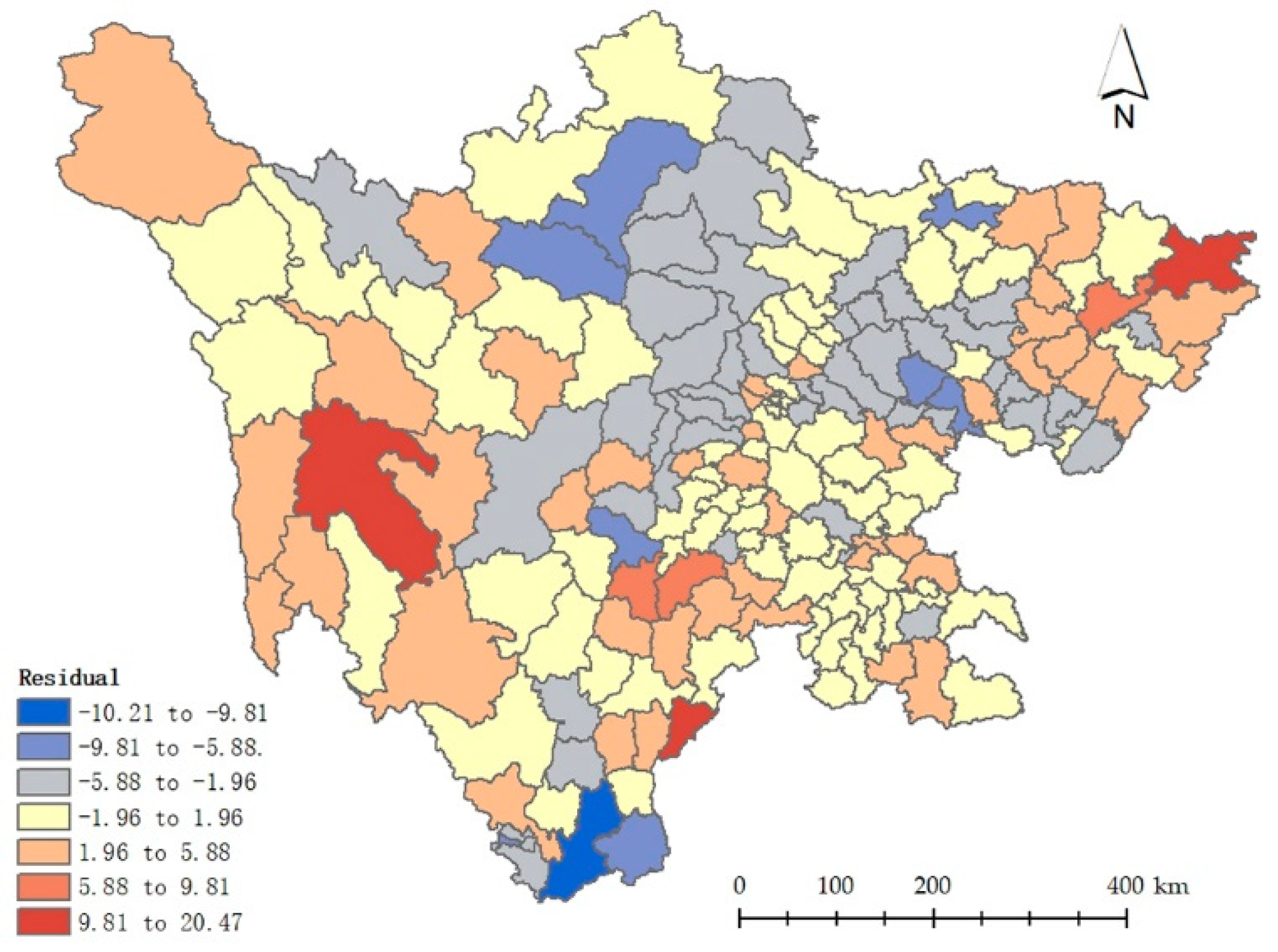
In Table 3, the variables T2, T3, and S4 with positive coefficients indicated that less warm and relatively high-slope areas are associated with poverty, while R, A4, and S1 with negative coefficients revealed that areas with more rain, at relatively high altitude, and relatively flat have lower poverty rates. All these results made sense. The adjusted R² was 0.59, indicating that the OLS model explained approximately 59% of the variation in the poverty rate by just six physical geographical variables. The Moran’s I of the residuals was 0.26 and the z-score was 5.79 (p < 0.01). The residuals of the OLS model shown in Figure 5 pointed to apparent spatial autocorrelation. However, as a global model, the OLS model was incapable of explaining some spatially correlated variabilities locally; we needed to select an alternative to better explore the relationship between the poverty rate and the independent variables. Since the local regression model can allow the regression coefficients to vary spatially [36], we needed to select a local regression model for the relationship between the poverty rate and geographic factors.

Figure 5. The residuals map of OLS model regression results.

5.2. GWR Model

The GWR model allows its coefficients to vary over the study area [33]. It helps understand the relationships between spatially unstable variables. The GWR model was formulated as:

$$P{O}_i={\beta }_{0i}+{\beta }_{1i}T2+{\beta }_{2i}T3+{\beta }_{3i}R+{\beta }_{4i}A4+{\beta }_{5i}S1+{\beta }_{6i}S4+{\epsilon }_i$$

where $P{O}_i$ is the poverty rate in county $i,$ and ${\beta }_{mi}$ are the estimated regression coefficients for the selected m variables from the OLS model about county $i$ in the study area. A series of related statistical tests were taken to examine whether an estimated local regression coefficient varies spatially [35]. A geographically weighted matrix $W_i$ was introduced to constrain the optimal solution of the GWR mode [36]:

$${\widehat{\beta }}_i={\left(X^T{W}_{i}X\right)}^{-1}{X}^T{W}_{i}Y$$

where $W_i$ is an n by n spatial weighting matrix as below:

$$W_i=\left(\begin{array}{ccccc}{w}_{i1}& 0& 0& \cdots & 0\\ 0& w_{i2}& 0& \cdots & 0\\ 0& 0& w_{i3}& \cdots & 0\\ ·& ·& ·& \cdots & ·\\ 0& 0& 0& \cdots & w_{in}\end{array}\right)$$

where n is the number of observations. Here, $w_{in}$ is the impact between location i and location n, and the values range between 0 and 1 [59]. In this study, spatially adaptive bandwidths were used.

6. Results

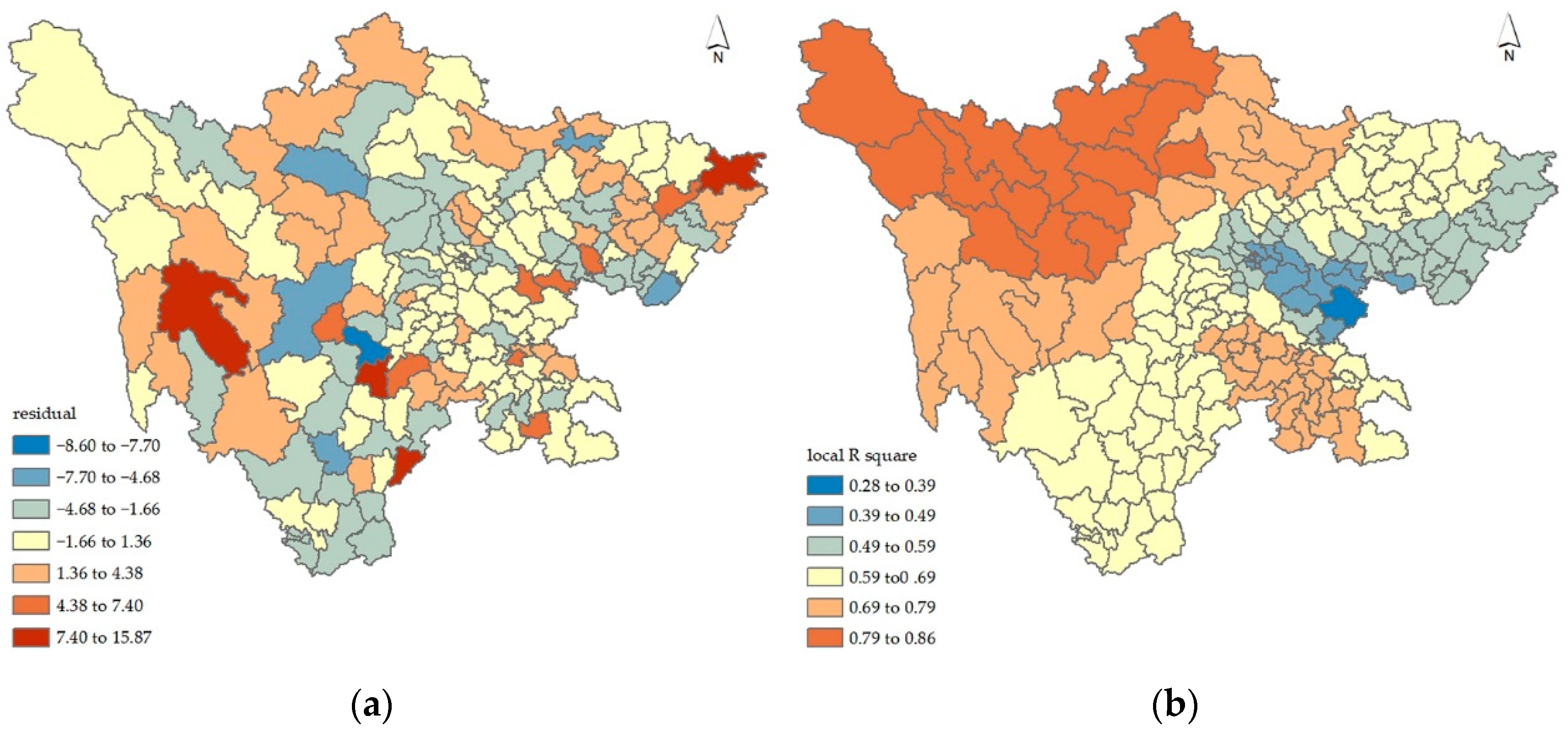
We utilized the GWR 4 package to perform the analysis. The results in Table 4 show that the GWR model was superior to the OLS model in terms of fitting the data. The overall R² = 0.76, the adjusted R² = 0.71, and AICc = 990.88. The results were much better than those of the OLS model (R² = 0.60, adjusted R² = 0.59, and AICc = 1036.37) in Table 3. The spatial distributions of the residuals and the local R² are displayed in Figure 6. Besides, the Moran’s I of the GWR model residuals = 0.02, and z-score = 0.47 (p-value = 0.64); this indicated that the spatial pattern of residuals showed no autocorrelation.

Table 4. Results of the GWR model and spatial dependence tests.

Variable	Min	25% Quartile	50% Quartile	75% Quartile	Max
Intercept	3.33	5.18	6.98	8.61	11.80
T2	−2.72	−0.44	0.42	1.11	2.59
T3	−1.38	1.06	1.67	2.85	4.40
R	−3.22	−2.38	−1.17	−0.15	1.52
A4	−2.42	−0.74	−0.10	2.05	9.72
S1	−2.65	−1.48	−1.35	−1.05	−0.43
S4	−0.39	0.93	1.80	2.27	2.78
Moran’s I (residuals)	0.02	-	-	-	-
R2	0.76	-	-	-	-
Adjusted R2	0.71	-	-	-	-
AICc	990.88	-	-	-	-

Figure 6. Spatial distributions of key results from the GWR model: (a) spatial distribution of residuals; (b) spatial distribution of local R² values.

In Figure 6b, we could see that the spatial distribution of local R² is not monotonic over the province. The counties in the northwest of the province had a high R² (up to 0.86), including Aba, Ganzi, Guangyuan, and Mianyang to Leshan, Yibin, Luzhou, and Zigong. The counties located in the east of the province had a low R², including Chengdu, Guang’an, Suining, and Ziyang. Most counties in the middle of the province had R² values in between. The clustering of R² values by different regions manifested the spatial effects of poverty rates regarding physical geographic features, indicating the advantage of GWR over OLS in revealing associations when regressing variables with spatial heterogeneity and spatial autocorrelation.

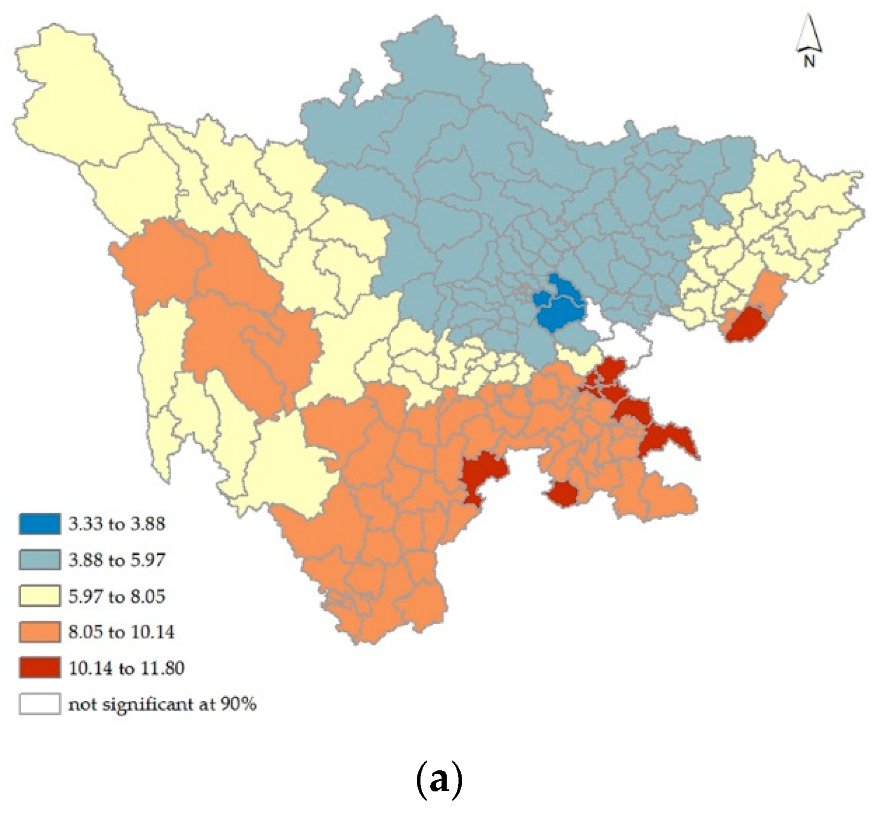
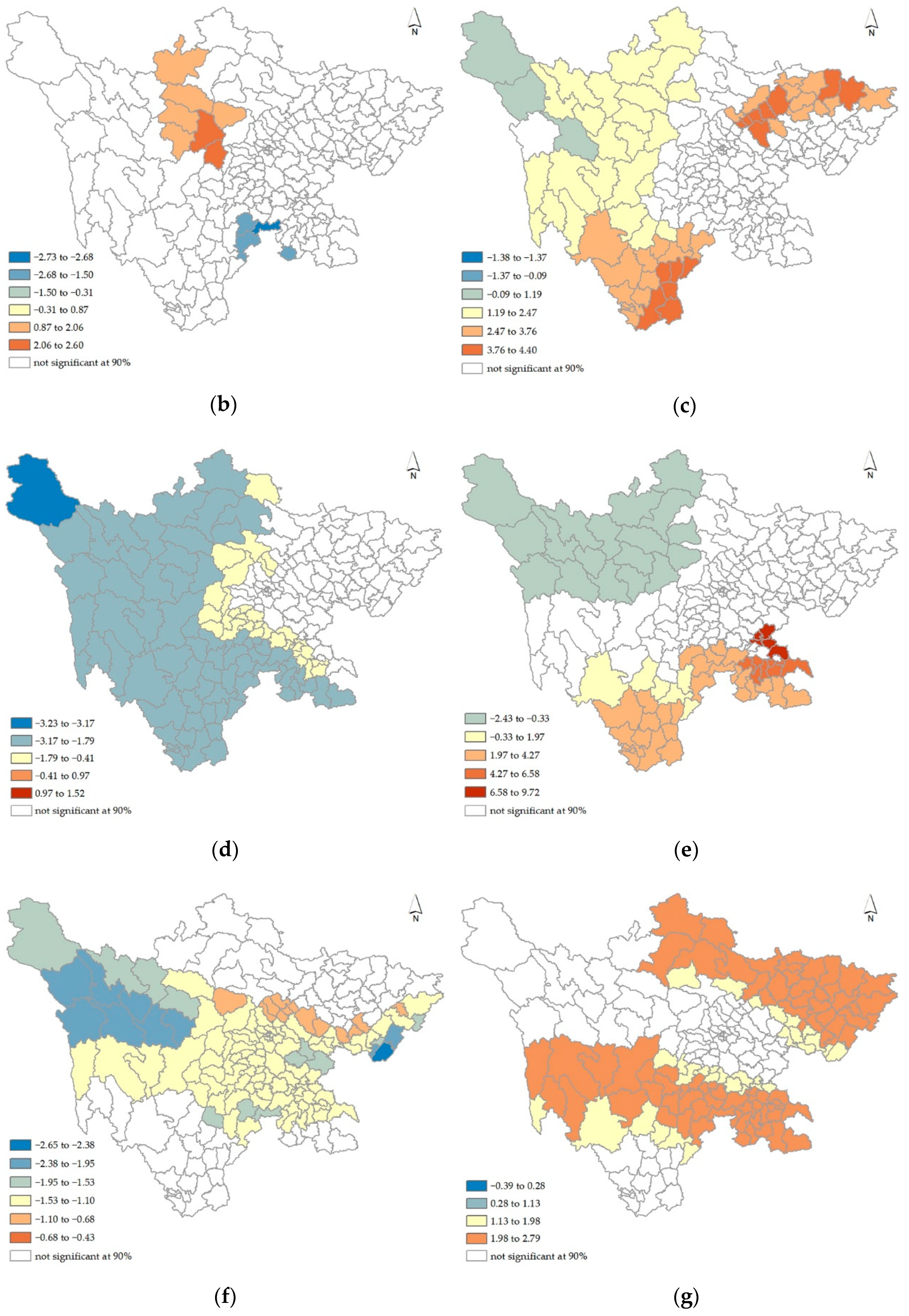
Figure 7 showed the spatial variation of the intercept and coefficients of independent variables from the GWR model. These maps were drawn using visualization methods in Mennis [60] and Matthews [61], including the modified classification method, standard deviation classification. The pseudo t values at the 90% significance level illustrate that the relationships between the dependent and each independent variable are not significant for some counties (in white color), meaning that the coefficients of each independent variable, regardless positive or negative, in these counties are meaningless [59].

Figure 7. Spatial distribution of Geographically Weighted Regression (GWR) regression coefficients: (a) intercept; (b) temperate rate 2 (T2); (c) temperature rate 3 (T3); (d) annual average rainfall (R); (e) altitude rate 4 (A4); (f) slope rate 1 (S1); (g) slope rate 4 (S4).

Specifically, we see that the intercept coefficients in Figure 7a were higher in the southeast of the province, mainly in Liangshan, Luzhou, Neijiang, and Yibin counties. This implied a generally higher poverty rate in these areas. Figure 7b shows that positive coefficients of temperature rate 2 (T2) were observed mainly for the northern counties Aba and Ya’an, and negative coefficients of T2 were mainly in the southeast counties Liangshan, Leshan, and Yibin. Positive coefficients between temperature rate 3 (T3) and the poverty rate were calculated for counties in the northeast, the south, and the west of the province, including Mianyang, Guangyuan, Bazhong, Dazhou, Liangshan, Panzhihua, Aba, and Ganzi, as shown in Figure 7c. Figure 7d shows annual average rainfall (R), with negative coefficients in the west and south of the Sichuan, including Aba, Ganzi, Ya’an, Liangshan, Meishan, Leshan, Yibin, and Zigong counties. Figure 7e presents altitude rate 4 (A4), with positive coefficients mainly in Liangshan, Panzhihua, Leshan, Yibin, Luzhou, and Neijiang counties and negative coefficients primarily for Aba and Ganzi counties. Slope rate 1 (S1) brought negative coefficients for counties in the middle of the province from the east to the west, as shown in Figure 7f. Slope rate 4 (S4) generated positive coefficients on both the north and south sides of the province, as shown in Figure 7g.

In summary, six variables of the GWR model were significant with positive and negative impacts on the poverty rate in the study area, and their associations with the poverty rate were spatially varied. The model helps us understand which and where physical geographic explanatory variables might have impacted poverty in Sichuan Province. It is important for smart and targeted policy-making for regional poverty reduction. Furthermore, these policies need to be adapted to local physical conditions.

7. Discussion

In this study, the global OLS regression model was able to generally capture the relationships between the poverty rate and the independent variables T2, T3, R, A4, S1, and S4. However, the OLS model results were not good enough in terms of discovering spatial variations. The six independent variables could only explain 59% of the spatial variety of the poverty rate, and the residuals showed obvious spatial autoregression. Comparatively, the local regression GWR model could characterize the independent variables’ spatial heterogeneity by their coefficients at the county level for the province. The six independent variables explained the spatial variation of the poverty rate by 71%, and the residuals had no spatial autoregression. Therefore, the GWR model was superior to the OLS model in this study [23,24,35].

Using GIS software, we can visually identify the spatial variation and significance of each independent variable coefficient. The study once again indicates that a local GWR-type regression model considering spatial dimension should be used rather than the general OLS regression model [58] for social and physical problems involving apparent spatial variations. For poverty research efforts, a good understanding of poverty’s spatial variations is key for making successful poverty-reduction policy making, implementation, and assessment.

In the selection of model variables, multicollinearity and significance are important selection criteria. Some variables have severe multicollinearity with others and need to be excluded from the regression analysis—for instance, RDLS, T1, T4, T5, TFH, TFM, TFL, LSH, LSM, LSL, DFH, DFM, DFL, A1, A2, A3, A5, S5, FR, DND, S2, and S3. Only T2, T3, R, A4, S1, and S4 were retained for the OLS and GWR regression analyses as significant variables. The fact that only six out of 28 variables were significant and, hence, selected by the models suggests, on the one hand, that definition and selection of variables are important, and on the other hand, significant variables need to be further explored [23,24,30,37,39].

8. Conclusions

In this paper, the associations between poverty and physical geographic factors were analyzed for the 183 counties of Sichuan province by using regression models and GIS software. We performed a Pearson correlation analysis and showed, in scatter plot matrices, an initial understanding of the relationship between each pair of variables, which include the dependent variable poverty rate and 28 physical geographic variables in seven groups. The OLS model was used to analyze the global regression relationships. Because the residuals of the model revealed spatial autocorrelation, the OLS model is considered unsuitable for describing the relationship between the poverty rate and physical geographic features. The GWR model was then applied to capture the spatial variations by county over the province and demonstrated its superiority [35].

We found that temperature rate 2 (T2), temperature rate 3 (T3), average annual rainfall (R), altitude rate 4 (A4), slope rate 1 (S1), and slope rate 4 (S4) had impacts on poverty rates in most counties [6,37,39], and the residuals of the model did not show spatial autocorrelation. The GWR model is more suitable for linking the poverty rate and physical geographic factors [23,24,30]. Furthermore, their relationships with poverty rate showed spatial heterogeneity. Specifically, the impact of temperature on poverty occurs in a specific temperature range, and it is necessary to improve the variety of crops or build facilities to improve the adaptability of agricultural production to temperature. As for the impact of precipitation on poverty, it is mainly the dry and hot river valleys in western Sichuan plateau areas on agricultural or animal husbandry production. Some altitudes and slopes had essential impacts on land use and transportation [13,14].

This research’s value lies in its exploratory findings on whether the persistent poverty problem is influenced by physical geographic factors as well as where and to what extent such influence by each factor exists [6,37]. Yet, more detailed investigations are much needed such as on the relationships between poverty rate and each factor group, for example, climate group, terrain group, or disaster group, and with other social and economic variables, including people’s perceptions and behaviors. Among many important research inquiries are the following: (1) What physical geographic factors can or should be modified to help reduce poverty? (2) Is mass relocating a population from poverty-prone locations to more affluent places a sound anti-poverty policy? (3) Why do people move or not move out of poverty regions, especially from severe ones, in terms of social, economic, cultural, religious, and institutional considerations? In short, we believe better modeled spatial variabilities, coupled with more socio-behavioral considerations in additional research, can better inform poverty reduction policy making, implementation, and assessment efforts for counties in Sichuan Province, its environs, and beyond. Moreover, from the perspective of ecology-economy-society coordinated development, this study can better promote regional sustainable development.

References

- Chinanews China Has Achieved Historic Achievements in the Five Years of Targeted Poverty Alleviation. Available online: https://www.chinanews.com/gn/2018/11-04/8667665.shtml (accessed on 1 September 2019).
- Bird, K.; Higgins, K.; Harris, D. Spatial Poverty Traps; Overseas Development Institute: London, UK, 2010. [Google Scholar]
- Montesquieu, C.d. The Spirit of Laws; Nourse and Vaillant: London, UK, 1748. [Google Scholar]
- Libby, O.G. Influences of Geographic Environment, on the Basis of Ratzel’s System of Anthropo-Geography. By Ellen Churchill Semple. (New York: Henry Holt and Company; London: Constable and Company. 1911. Pp. xvii, 683.). Am. Hist. Rev. 1912, 17, 355–357. [Google Scholar] [CrossRef]
- Huntington, E. Civilization and Climate; Yale University Press: London, UK, 1924. [Google Scholar]
- Thompson, J.H. What About a Geography of Poverty? Econ. Geogr. 1964, 40, i. [Google Scholar] [CrossRef]
- Elgie, R.A.; Ulch, C.L. The Geography of Poverty in the United States. Econ. Geogr. 1973, 49, 3. [Google Scholar] [CrossRef]
- Shaw, W. The Geography of United States Poverty: Patterns of Deprivation, 1980–1990; Garland Pub: New York, NY, USA, 1996; ISBN 9780815325369. [Google Scholar]
- Pringle, D.G.; Walsh, J.; Hennessy, M. Poor People, Poor Places: The Geography of Poverty and Deprivation in Ireland; Oak Tree Press: Dublin, Ireland, 1999; ISBN 1860761089. [Google Scholar]
- Shaw, M. Poor People, Poor Places: A Geography of Poverty and Deprivation in Ireland. J. Rural Stud. 2001, 17, 131–132. [Google Scholar] [CrossRef]
- Pacione, M. The geography of multiple deprivation in Scotland. Appl. Geogr. 1995, 15, 115–133. [Google Scholar] [CrossRef]
- Bramley, G.; Lancaster, S.; Gordon, D. Benefit Take-up and the Geography of Poverty in Scotland. Reg. Stud. 2000, 34, 507–519. [Google Scholar] [CrossRef]
- Jyotsna, J.; Mlartin, R. Spatial Poverty Traps? (Enlish); Policy Research Working Papers Series 1862; The World Bank: Washington, DC, USA, 1997. [Google Scholar]
- Jalan, J.; Ravallion, M. Geographic poverty traps? A micro model of consumption growth in rural China. J. Appl. Econom. 2002, 17, 329–346. [Google Scholar] [CrossRef]
- Straubhaar, T.; Suhrcke, M.; Urban, D.M. Divergence—Is It Geography? HWWA Discussion Papers 181; Hamburg Institute of International Economics (HWWA): Hamburg, Germany, 2002. [Google Scholar]
- Bloom, D.E.; Canning, D.; Sevilla, J. Geography and Poverty Traps. J. Econ. Growth 2003, 8, 355–378. [Google Scholar] [CrossRef]
- Paraguas, F.J.; Kamil, A.A. Spatial econometrics modeling of poverty. WSEAS Trans. Math. 2005, 4, 368. [Google Scholar]
- Deinne, C.E.; Ajayi, D.D. Spatial Dynamics of Urban Poverty in Delta State Nigeria. J. Poverty 2017, 22, 1–18. [Google Scholar] [CrossRef]
- Hu, Y.; Fang, Y.; Jiang, W. Spatial Correlation and Interaciton between Rocky Desertification and Poverty in Karst Mountainous Area in Guangxi. Resour. Ind. 2009, 11, 105–110. [Google Scholar]
- Wang, S.; Tian, J.; Wang, B.; Cheng, L.; Du, G. Regional Characteristics and Causes of Rural Poverty in Northeast China from the Perspective of Targeted Poverty Alleviation. Sci. Geogr. Sin. 2017, 37, 1449–1458. [Google Scholar]
- Zhao, Y.; Liu, X.; Guo, Y. Model Analysis for Spatial Poverty in the Poor Areas of Liupan Mountain in Ningxia Hui Autonomous Region Based on GIS. Res. Soil Water Conserv. 2014, 21, 94–99. [Google Scholar]
- Ma, Z.; Chen, X.; Jia, Z.; Lv, P. Poor people, or poor area? A geostatistical test for spatial poverty traps. Geogr. Res. 2018, 37, 1997–2010. [Google Scholar]
- Tong, X.; Liang, Q.; Wei, Y.; Liu, Q. Analysis of Influencing Factors of County Poverty in Guangxi Based on Geo Detector. Hunan Agric. Sci. 2018, 82–88. [Google Scholar] [CrossRef]
- Ding, J.; Leng, Z. Regional poverty analysis in a view of geography science. Acta Geogr. Sin. 2018, 73, 232–247. [Google Scholar]
- Liu, Y.; Liu, J.; Zhou, Y. Spatio-temporal patterns of rural poverty in China and targeted poverty alleviation strategies. J. Rural Stud. 2017, 52, 66–75. [Google Scholar] [CrossRef]
- Niu, T.; Chen, Y.; Yuan, Y. Measuring urban poverty using multi-source data and a random forest algorithm: A case study in Guangzhou. Sustain. Cities Soc. 2020, 54, 102014. [Google Scholar] [CrossRef]
- Haughton, J.; Khandker, S.R. Understanding the Determinants of Poverty. In Handbook on Poverty and Inequality; The World Bank: Washington, DC, USA, 2009; pp. 145–158. [Google Scholar]
- Xhafaj, E.; Nurja, I. Determination of the Key Factors that Influence Poverty through Econometric Models. Eur. Sci. J. 2014, 10, 65–72. [Google Scholar]
- Duarte, R. Socioeconomic Determinants of Poverty in Paraguay; Washington University in St. Louis: St. Louis, MO, USA, 2015. [Google Scholar]
- Petrucci, A.; Salvati, N.; Seghieri, C. Autologistic Regression Model for Poverty Mapping and Analysis. Metodoloski Zv. 2004, 1, 225–234. [Google Scholar]
- Achia, T.N.O.; Wangombe, A.; Khadioli, N. A logistic regression model to identify key determinants of poverty using demographic and health survey data. Eur. J. Soc. Sci. 2010, 13, 38–45. [Google Scholar]
- Karim, A.; Noy, I. Poverty and Natural Disasters: A Meta-Regression Analysis. Rev. Econ. Inst. Econ. Soc. Ist. 2016, 7, 1–26. [Google Scholar] [CrossRef]
- Brunsdon, C.; Fotheringham, A.S.; Charlton, M.E. Geographically Weighted Regression: A Method for Exploring Spatial Nonstationarity. Geogr. Anal. 1996, 28, 281–298. [Google Scholar] [CrossRef]
- Brunsdon, C.; Fotheringham, S.; Charlton, M. Geographically weighted regression-modelling spatial non-stationarity. J. R. Stat. Soc. Ser. D (Stat.) 1998, 47, 431–443. [Google Scholar] [CrossRef]
- Fotheringham, A.S.; Brunsdon, C.; Charlton, M. Quantitative Geography: Perspectives on Spatial Data Analysis; Sage: London, UK, 2000. [Google Scholar]
- Fotheringham, A.S.; Brunsdon, C.; Charlton, M. Geographically Weighted Regression: The Analysis of Spatially Varying Relationships; John Wiley & Sons: Hoboken, NJ, USA, 2002. [Google Scholar]
- Benson, T.; Chamberlin, J.; Rhinehart, I. An Investigation of the Spatial Determinants of the Local Prevalence of Poverty in Rural Malawi. Food Policy 2005, 30, 532–550. [Google Scholar] [CrossRef]
- Dawson, T.; Sandoval, J.S.; Sagan, V.; Crawford, T.; Dawson, T.; Sandoval, J.S.O.; Sagan, V.; Crawford, T. A Spatial Analysis of the Relationship between Vegetation and Poverty. ISPRS Int. J. Geo-Inf. 2018, 7, 83. [Google Scholar] [CrossRef]
- Wang, Y.; Wang, M.; Wu, D.; Zhao, L.; Ding, J. Spatial Patterns and Determinants of Rural Poverty: A Case of Guizhou Province, China. Sci. Geogr. Sin. 2017, 37, 217–227. [Google Scholar]
- Vaziri, M.; Acheampong, M.; Downs, J.; Rafee Majid, M. Poverty as a function of space: Understanding the spatial configuration of poverty in Malaysia for Sustainable Development Goal number one. GeoJournal 2019, 84, 1317–1336. [Google Scholar] [CrossRef]
- Guo, Y.; Chang, S.S.; Sha, F.; Yip, P.S.F. Poverty concentration in an affluent city: Geographic variation and correlates of neighborhood poverty rates in Hong Kong. PLoS ONE 2018, 13, 1–17. [Google Scholar] [CrossRef]
- Robinson, C.; Bouzarovski, S.; Lindley, S. Underrepresenting neighbourhood vulnerabilities? The measurement of fuel poverty in England. Environ. Plan. A Econ. Space 2018, 50, 1109–1127. [Google Scholar] [CrossRef]
- Lucas, K.; Philips, I.; Mulley, C.; Ma, L. Is transport poverty socially or environmentally driven? Comparing the travel behaviours of two low-income populations living in central and peripheral locations in the same city. Transp. Res. Part A Policy Pract. 2018, 116, 622–634. [Google Scholar] [CrossRef]
- Sichuan Yearbook Office. Sichuan Yearbook; Ma, X., Ed.; Sichuan Yearbook Society: Chengdu, China, 2017. [Google Scholar]
- Sichuan Statistical Bereau; NBS Survey Office in Sichuan. Sichuan Statistical Yearbook 2019; China Statistics Press: Beijing, China, 2019.
- Sichuan Statistics Bureau Population Statistics Bulletin of Sichuan Province in 2018. Available online: http://web.sctjj.cn/sjfb/tjgb/201903/t20190319_277120.html (accessed on 10 September 2019).
- Sichuan Provincial Committee of the Communist Party of China Decision on Commending Advanced Cities and Counties for Poverty Alleviation in 2016. Sichuan Dly. 2017. Available online: https://epaper.scdaily.cn/shtml/scrb/20170423/161450.shtml (accessed on 22 September 2019).
- Li, M.; Hou, C. 45 Poverty-Stricken Counties Reduced Poverty by 446,000 in Three Years. Sichuan Dly. 2017. Available online: https://epaper.scdaily.cn/shtml/scrb/20170816/171006.shtml (accessed on 22 September 2019).
- Gallup, J.L.; Sachs, J.D. Agriculture, climate, and technology: Why are the tropics falling behind? Am. J. Agric. Econ. 2000, 82, 731–737. [Google Scholar] [CrossRef]
- Yang, J. A GWR-Based Study on Impoveriishment Factors of Guizhou Province: A Case Study of Jianhe County; Guizhou University: Guiyang, China, 2018. [Google Scholar]
- Zhao, Y. Research on the Spatial Poverty Trap of Concentrated Contiguous Area with Particular Difficulties on Basis of the Geographic Capital; Ningxia University: Yinchuan, China, 2015. [Google Scholar]
- Akoglu, H. User’s guide to correlation coefficients. Turkish J. Emerg. Med. 2018, 18, 91–93. [Google Scholar] [CrossRef]
- Wheeler, D.; Tiefelsdorf, M. Multicollinearity and correlation among local regression coefficients in geographically weighted regression. J. Geogr. Syst. 2005, 7, 161–187. [Google Scholar] [CrossRef]
- Garg, A.; Tai, K. Comparison of statistical and machine learning methods in modelling of data with multicollinearity. Int. J. Model. Identif. Control 2013, 18, 295. [Google Scholar] [CrossRef]
- Liu, R.X.; Kuang, J.; Gong, Q.; Hou, X.L. Principal component regression analysis with SPSS. Comput. Methods Programs Biomed. 2003, 71, 141–147. [Google Scholar] [CrossRef]
- Wong, D.W.-S.; Lee, J. Statistical Analysis of Geographic Information with ArcView GIS and ArcGIS; John Wiley & Sons: Hoboken, NJ, USA, 2005. [Google Scholar]
- Wong, D.W.S.; Wang, F. Spatial Analysis Methods. In Comprehensive Geographic Information Systems; Huang, B., Ed.; Elsevier: Amsterdam, The Netherlands, 2018; pp. 125–147. [Google Scholar]
- Xu, Y.; Wang, L. GIS-based analysis of obesity and the built environment in the US. Cartogr. Geogr. Inf. Sci. 2015, 42, 9–21. [Google Scholar] [CrossRef]
- Lin, C.-H.; Wen, T.-H.; Lin, C.-H.; Wen, T.-H. Using Geographically Weighted Regression (GWR) to Explore Spatial Varying Relationships of Immature Mosquitoes and Human Densities with the Incidence of Dengue. Int. J. Environ. Res. Public Health 2011, 8, 2798–2815. [Google Scholar] [CrossRef]
- Mennis, J. Mapping the results of geographically weighted regression. Cartogr. J. 2006, 43, 171–179. [Google Scholar] [CrossRef]
- Matthews, S.A.; Yang, T.-C. Mapping the results of local statistics: Using geographically weighted regression. Demogr. Res. 2012, 26, 151–166. [Google Scholar] [CrossRef]
Publisher’s Note: MDPI stays neutral with regard to jurisdictional claims in published maps and institutional affiliations. |
© 2020 by the authors. Licensee MDPI, Basel, Switzerland. This article is an open access article distributed under the terms and conditions of the Creative Commons Attribution (CC BY) license (http://creativecommons.org/licenses/by/4.0/).