Abstract
Impact assessments on climate change are essential for the evaluation and management of irrigation water in farming practices in semi-arid environments. This study was conducted to evaluate climate change impacts on water productivity of maize in farming practices in the Lower Chenab Canal (LCC) system. Two fields of maize were selected and monitored to calibrate and validate the model. A water productivity analysis was performed using the Soil–Water–Atmosphere–Plant (SWAP) model. Baseline climate data (1980–2010) for the study site were acquired from the weather observatory of the Pakistan Meteorological Department (PMD). Future climate change data were acquired from the Hadley Climate model version 3 (HadCM3). Statistical downscaling was performed using the Statistical Downscaling Model (SDSM) for the A2 and B2 scenarios of HadCM3. The water productivity assessment was performed for the midcentury (2040–2069) scenario. The maximum increase in the average maximum temperature (Tmax) and minimum temperature (Tmin) was found in the month of July under the A2 and B2 scenarios. The scenarios show a projected increase of 2.8 °C for Tmax and 3.2 °C for Tmin under A2 as well as 2.7 °C for Tmax and 3.2 °C for Tmin under B2 for the midcentury. Similarly, climate change scenarios showed that temperature is projected to decrease, with the average minimum and maximum temperatures of 7.4 and 6.4 °C under the A2 scenario and 7.7 and 6.8 °C under the B2 scenario in the middle of the century, respectively. However, the highest precipitation will decrease by 56 mm under the A2 and B2 scenarios in the middle of the century for the month of September. The input and output data of the SWAP model were processed in R programming for the easy working of the model. The negative impact of climate change was found under the A2 and B2 scenarios during the midcentury. The maximum decreases in Potential Water Productivity (WPET) and Actual Water Productivity (WPAI) from the baseline period to the midcentury scenario of 1.1 to 0.85 kgm−3 and 0.7 to 0.56 kgm−3 were found under the B2 scenario. Evaluation of irrigation practices directs the water managers in making suitable water management decisions for the improvement of water productivity in the changing climate.
1. Introduction
Climate change is a real threat to agriculture and food security, and it has caused a shortage of water worldwide [1,2]. Variation in temperature, uneven distribution of precipitation, and untimely floods have affected the water resources in Pakistan [3]. Different studies show that the uncertainties in climate change decreased the per capita water availability from 5300 m3 in the 1950s to 1000 m3 in 2011, and successive decreases are expected to continue in the future, from 855 m3 in 2020 to 769 m3 in 2050 [4]. Reduced water supplies in the changing climate would, thus, pose a serious threat to food security in the near future. As climate change is enhancing water scarcity in the arid and semi-arid regions of the world [5,6], including Pakistan, efficient management of water resources is crucial to meet crop water requirements [7,8].
Maize is the most important food and forage crop in the world [9]. The production area for maize is the third largest in Pakistan after wheat and rice. Its shares in value-added agriculture (VAA) and gross domestic product (GDP) are 2.1% and 0.4%, respectively. Still, there is a big difference between the actual and potential yields of maize in the ideally considered environment of Pakistan due to the improper use of water and fertilizer [10]. Improper irrigation scheduling has resulted in 30–96% and 28–32% reduction in the yield and biomass production, respectively, of maize crops [11,12]. As maize is also sensitive to water stagnation, the increase in rainfall intensity due to changing climate is a real threat to the ideal climatic conditions of the maize crop in Pakistan. Agricultural production will be impacted by climate change from the regional to the global scale based on the research studies carried out at local, regional, and global levels [13,14,15].
Studies on maize production show variations in the yield under different treatments and levels of fertigation and irrigation scheduling. Huang et al. [16] described a reduction in maize yield in a semi-arid environment due to changes in temperature and variations in the rainfall intensity. Bergamaschi et al. [17] found a significant decrease in maize yield due to rainfall uncertainty. Lobell et al. [18] revealed a reduction in yield from 1.7% to 1% as the temperature exceeded 30 °C under water-stressed conditions. Ahmad et al. [19] revealed a 43% reduction in maize yield resulting from a minimum temperature increase of 2.2 °C and maximum of 4.4 °C. Abbas et al. [20] found a potential decrease in yield due to changes in maize phenology under changing climate.
Soil–Water–Atmosphere–Plant (SWAP) is an ecohydrological model that is used to estimate crop yield, transpiration, evapotranspiration, and percolation [21]. The SWAP model can evaluate the system at different spatio-temporal scales based on field measurements [21]. The projected global warming is likely to disturb hydrological systems and eventually change the occurrence of extreme events and disturb the dynamics of water availability [22]. However, the trend of climate change impact on hydrological systems varies from region to region. Due to the complexity in hydrological systems, most climate change studies have fixated on temperature, precipitation, and evapotranspiration [23]. In the last two decades, hydrological and General Circulation Models (GCMs) were coupled to project the climate change impact on the water resources of a watershed. GCMs are important and recent tools for regional- to global-scale analyses of climatic parameters like minimum and maximum temperature and rainfall. These models are numerically coupled and represent the global system, i.e., atmosphere, ocean, and sea ice [24]. Due to the coarse spatial resolution, downscaling techniques, i.e., statistical and dynamical, have been developed for use in GCMs at the regional scale [25,26,27]. Statistical downscaling techniques aid in developing the relation between GCM and observed variables [22]. The climate scientific community has widely adopted statistical downscaling due to its faster and inexpensive computation [27].
The agricultural perspective of food security requires more crops per drop of water applied in the field in the changing climate. Assessment of water productivity is the evaluative indicator for irrigation system performance in farmers’ practices. Water productivity is considered as a water-saving indicator at different stages of utilization in the agricultural sector [28]. Molden and Rust [29] defined water productivity at different stages of water utilization. The purpose of this study was to quantify the impact of climate change on water productivity of the maize crop under irrigated conditions and evaluate the irrigation system performance under the changing climate.
2. Methodology
2.1. Research Sites
The study was performed in the Lower Chenab Canal (LCC) system in the Punjab province of Pakistan, as shown in Figure 1. Two farmers’ fields were selected and extensively monitored in the LCC, represented as MZ1 and MZ2. The LCC command is the oldest and largest canal water distribution system in Punjab, Pakistan, and it is a true representative of the irrigation system of Pakistan. The mean historical maximum and minimum temperatures during the autumn season are 35 and 21 °C, respectively. The maximum sunshine duration during this season is almost twelve hours. Maize is the third major crop of the study area, following wheat and rice [30]. In the autumn season, maize is sown from mid-July to mid-August and harvested from the end of October to the middle of December.
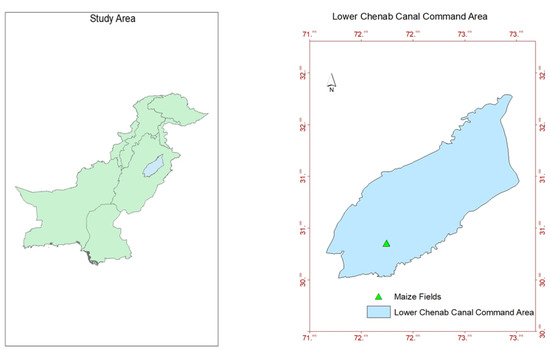
Figure 1.
Research sites in the Lower Chenab Canal system.
2.2. Climate Change Scenarios
In this research, the most widely used GCM, the Hadley Center Coupled Model version 3 (HadCM3) (Hadley Centre, Exeter, UK), was used. HadCM3 is considered as the major important GCM in the development of the Third and the Fourth Assessment reports of the Inter-Governmental Panel on Climate Change (IPCC) [31]. HadCM3 is successfully applied for the attribution, prediction, climate detection, and sensitivity analyses in climatic research. HadCM3 is still considered as a highly ranked GCM compared to others because it does not use flux adjustment and it decently simulates of the present climate. It can also capture the time-reliant patterns of past climate change in reaction to anthropogenic and natural forcing [32]. The global frame of HadCM3 has been divided into a grid for the ease of data acquisition by portioning it into seven subframes. The portions are based on the significant representation of land area and land–sea boundaries as defined according to its land–sea cover. Data of the HadCM3 predictors were acquired from the site-representative X and Y grid from the Canadian website http://climate-scenarios.canada.ca/index.php?page=pred-hadcm3&wbdisable=true. A total of 26 predictors of the National Centers for Environmental Prediction (NCEP) and HadCM3 (H3A2 and H3B2) from 1961–2001 and 1961–2099 were downloaded, respectively.
2.2.1. Statistical Downscaling of GCM Data
In statistical downscaling, large-scale climatic conditions describe the regional climate based on local physical environmental features. The Statistical Downscaling Model (SDSM) (Department of Geography, Loughborough Unuiversity, Loughborough, UK), developed by Wilby et al. [33], is based on Multiple Linear Regression and Stochastic Weather Generator. SDSM has been used extensively all over the globe [34] for downscaling precipitation, temperature and evaporation. In the current study, SDSM was used to downscale HadCM3 A2 and B2 scenarios for the maximum and minimum temperature and precipitation for the duration of 2011–2099 in the LCC command area. SDSM approaches are quicker and have lower computational costs; therefore, SDSM methods have been extensively approved by the technical community working on climate [35]. The A2 scenario models a diverse world with very relaxed regulations throughout regions, an unceasing growth in worldwide population, locally driven economic development, extra uneven fiscal development per person, and a rapid change and increase in technology as compared to the other scenarios. Conversely, the B2 scenario highlights the global importance on socio-environmental sustainability and models an indigenous way to carry out economic growth. In the B2 scenario, the world population will be lower, as compared to A2, with intermediate development in economic growth. B2 also models more diverse changes in technology at a slower rate compared to other scenarios, i.e., A1 and B1 [36].
2.2.2. Bias Correction
In this study, to remove biases from the daily temperature and rainfall downscaled data, Bias Correction (BC) was performed by following the methods of Salzmann et al. [37] and Mahmood and Babel [38]. In this technique, first, biases are estimated by subtracting the mean monthly observed data from the mean monthly simulated data. Then, future daily simulated data are corrected based on their respective monthly de-biased factors.
A mathematical representation for the estimation of biases is given below (Equations (1) and (2)) to de-bias the daily temperature and rainfall data, respectively:
where Tdb and Rdb are the future de-biased daily data of temperature and precipitation, respectively. Tsdf and Rsdf represent SDSM-based downscaled data for the duration of 2011–2099, and Tsdp and Rsdp represent SDSM-based downscaled data for the baseline period 1980–2010. and are the mean monthly values of temperature and rainfall, respectively, for the 31-year SDSM base period. and represent the mean monthly observed values for temperature and rainfall for the 31 years.
Precipitation variability is affected by its frequency and intensity [39]. In the application of SDSM, precipitation quantity, and not in the frequency, is highlighted, and any methodological errors due to SDSM-based downscaling must be eliminated. In the case of frequency, it is assumed that SDSM is precise.
2.3. Soil-Water-Atmosphere-Plant (SWAP) Model
SWAP version 3.0 (Wageningen University and Research, Wageningen, The Netherlands) was coupled with GCM output using R to assess climate change impact. SWAP is an ecohydrological model based on deterministic and physical laws vital to biochemical and hydrological processes occurring in the continuum of soil, water, plant, and atmosphere [40]. SWAP simulates vertical soil water flow and salt transport in close interaction with crop growth. Richards’ equation [41] is used to compute the transient soil water flow in Equation (3) below:
where Cw is the differential soil water capacity (L1), h is the soil water pressure head (L), K is the hydraulic conductivity (L T1), Sa is the rate of root water extraction (T1), and z is the vertical coordinate (L) (positive upward). The numerical solution of Equation (3) is based on defined initial and boundary conditions, and relationships between soil hydraulic variables such as soil moisture (), pressure head (h), and hydraulic conductivity (K) are needed. The following relations between these variables have been used [42,43]:
where res is the residual water content (L3 L−3), the saturated water content (L3 L−3), is the relative saturation (–), an empirical shape factor (L−1), n is an empirical shape factor (–), is the saturated hydraulic conductivity (L T−1), and l is an empirical coefficient (–).
Salt transport in the soil profile mainly is due to convention, diffusion, and dispersion. The diffusion process under irrigated conditions is too slow, and in this study it was neglected. A convection–dispersion equation, Equation (6), was applied for salt transport [44,45]:
Equation (6) is valid for dynamic, one-dimensional, and convective–dispersive salt transport, and it simulates the reduction of root water uptake caused by salt stress in unsaturated/saturated soils. SWAP numerically solves Equation (6) using a defined initial salt concentration and concentration of salts via irrigation.
2.3.1. Data Collection for the Calibration and Validation of the SWAP Model
In this study, soil sampling was performed up to a depth of 120 cm. Sampling intervals of 0–15, 15–30, 30–60, 60–90, and 90–120 cm were selected for the comprehensive analysis of the required parameters. Soil salinity was measured by a 1:2 soil–water suspension using a conductivity meter. Similarly, the physical properties of soil were analyzed using standard methods, i.e., soil texture using the international pipette method [46], United States Department of Agriculture (USDA) classification, bulk density using the core method, saturated and residual soil moisture using the gravimetric method, and hydraulic conductivity using the constant water head method [47].
2.3.2. Input Parameters of the SWAP Model
Most of the SWAP input parameters were directly measured in the laboratory and field. Two farmers’ fields, represented as MZ1 and MZ2, were monitored in the LCC area for measurements of the soil-water and crop data. In the LCC, maize sowing is practiced twice a year. SWAP input parameters could be grouped to define the initial conditions, upper and lower boundary conditions, and also the detailed characteristics of crop and soil.
The rainfall, potential evapotranspiration (ETp), and irrigation define the upper boundary of the soil profile. The Penman–Monteith equation was used to estimate ETp using daily meteorological data. For the lower boundary condition, free drainage conditions were applied due to the deep groundwater level greater than 3 m depth from the soil surface [28]. Initial conditions of the salinity and soil moisture were directly measured from the fields.
The crop parameters were estimated based on multiple field observations, i.e., stages of crop development (emergence, anthesis, maturity, and harvest), number of tillers, plant density and height, dry matter, and yield. Leaf area index was measured using the leaf area meter. The crop height and rooting depth were prescribed as a function of crop development stage, which was assumed to be linear in time from emergence to harvest [28]. Considering the less optimal farming practices of the farmers, crop parameters such as light use efficiency ε (kg ha−1 hr−1/ J m2 s−1) and maximum CO2-assimilation rate A (kg ha−1 hr−1) were considered as decreasing based on the crop measurements [21]. The various input parameters used are summarized in Table 1.

Table 1.
Main crop parameters specified for the SWAP model.
2.3.3. Soil Hydraulic Parameters: Inverse Modeling
In this study, only the upper 300 cm of the soil column was considered for simulation, as most of the desired hydrological processes occur in the upper soil column. The soil column was divided into three soil layers based on the measured soil profile up to 120 cm, and the last observed soil characteristics were given to the depth of 120–300 cm soil layer. The soil column was further divided into 40 parts, with a width of 1 cm for the top 10 parts, then 5 cm for the succeeding 10 parts, and 10 cm for the remaining soil column. For salt transport in the irrigated field, the dispersion length Ldis was set to 5 cm [48]. Furthermore, a coefficient of 0.35 cm d−1, according to [49], was used to reduce the rate of evaporation from the soil. In this study, the methods of Singh et al. [28] were followed by linking the parameter estimation technique (PEST) with the SWAP model.
2.4. Water Productivity Assessment
In the system of crop production, water productivity (WP) is defined as the crop yield per unit amount of water used [50]. Additionally, WP is defined in different ways by different stockholders, referring to different types of yield from crop production system (dry matter or grain yield) and amount of water consumed (transpiration, evapotranspiration, and irrigation) [29]. Actual evapotranspiration (ETa) represents the actual amount of water required for crop production, and the consumed water via ETa is not reusable for the crop production system. It must be used as productively as possible, and it is logical to express potential water productivity as (). The inevitable loss of water due to evaporation decreases water productivity from the ideal water productivity () to WPET. However, in reality, percolation losses increase the denominator in the expression of WP, hence decreasing the WP from WPET to actual water productivity (). Climate change impact assessments were performed on each level of the defined water productivity hierarchy. This assessment was performed for the baseline (1980–2010) and midcentury periods (2040–2069) under the A2 and B2 scenarios for both maize fields, as shown in Figure 2.
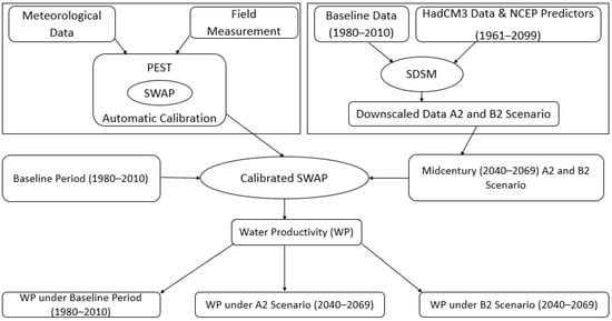
Figure 2.
Flow diagram of the methodology.
3. Results and Discussion
3.1. Optimized Soil Hydraulic Parameters of SWAP
The measured soil moisture and soil salinity from the farmers’ fields were used to optimize the soil hydraulic parameters with automatic calibration using the parameter estimation technique (PEST). PEST inverse solution optimizes the α and n for the different soil layers. Uniqueness of the solution was obtained when iterations in the inverse solution with different initial constraints of α and n resulted in the same values [28]. Table 2 shows the optimized values of α and n along with Ks, θs, and θr that were used in the SWAP.
Table 2.
Optimized soil hydraulic parameters for the maize fields.
3.2. Calibration and Validation of SWAP
The measured soil-water and crop data from the monitored maize fields MZ1 and MZ2 were used in the calibration and the validation of the SWAP. Calibration was performed from mid-July to the end of August, and validation was performed from the start of September to crop harvest. A graphical representation of the MZ1 field is given in Figure 3.
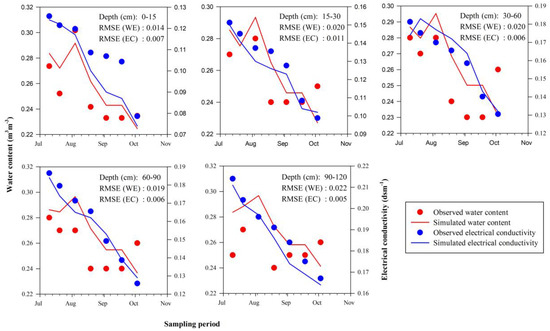
Figure 3.
Graphical representation of the calibration and validation of MZ1 field (RMSE is the Root Mean Squre Error, WE is the Water Content and EC is Electrical Conduvtivity).
Figure 3 shows the measured and simulated soil moisture and soil salinity during the calibration and validation periods, respectively. The results showed good agreement between the simulated and observed moisture content and the electrical conductivity (EC) during the calibration and validation periods. The maximum Root Mean Squre Error (RMSE) of the moisture content was 0.022 during the validation period. The maximum RMSE for the EC was 0.010 during the calibration period of MZ2. Details of the statistical analyses for all samples are presented in Table 3.
Table 3.
Statistical analysis of the SWAP model during calibration and validation.
3.3. Future Climatic Data under A2 and B2 Scenarios
The highest increase in the average minimum and maximum temperatures, 2.8 °C and 3.3 °C respectively, was found for the month of July under the A2 scenario. While under the B2 scenario, the highest increase in temperature was also found in the month of July, with a maximum increase of 3.2 °C and minimum 2.7 °C. A decrease in temperature was also found during the study period, and maximum decrease in the average maximum and minimum temperatures, 7.7 °C and 6.8 °C respectively, was found under the B2 scenario. The rainfall trend showed a significant decrease during the study period, as the average annual rainfall of the study area was about 400 mm [51]. The highest decrease in rainfall was 56 mm under both A2 and B2 scenarios during the month of September. Detailed changes in the climatic parameters are presented in Table 4.
Table 4.
Maximum and minimum temperature and precipitation changes under A2 and B2 midcentury scenarios.
3.4. Climate-Induced Salt and Water Balances
In this study, significant groundwater recharge variations were found, as shown in Table 5. This possibly was due to heavy irrigation during the maize cropping season. Heavy rainfall left the soil wet; thus, less water was required for application.
Table 5.
Simulation of groundwater recharge and soil salinity built up.
Groundwater recharge variations for the baseline period were found to be significant. Negative values indicate depletion of the aquifer. Depletion of the aquifer was high due to higher crop water demand in the maize season (July to October). This showed a higher rate of groundwater extraction for the months of July to October. In this period, irrigation water availability from the irrigation network was at its peak, and the occurrence of rainfall was also at maximum due to the monsoon period.
Salt accumulation was found to increase as the groundwater recharge rate decreased. For the midcentury A2 scenario, the groundwater recharge rate was also found higher. The average mean recharge was increased midcentury as compared to the baseline period. Similarly, this increase in rainfall reduced the mean average salt accumulation during the A2 midcentury scenario. While the groundwater recharge in the midcentury was reduced, as compared to the baseline period, due to the significant decrease in rainfall during the monsoon season.
Similarly, under the B2 scenario for the midcentury, variations in the groundwater recharge and salt accumulation were found. Groundwater recharge was found to increase as compared to the baseline period. It further reduced aquifer depletion due to the higher rate of groundwater pumping, as rainfall intensity increased the groundwater recharge rate and also leached down the salts from the root zone. Under the B2 scenario, groundwater recharge was less like the A2 scenario due to the decrease in rainfall during the monsoon season (Table 5).
3.5. Climate-Induced Water Productivity
In this study, flood irrigation was the main method, and no effects of other improved irrigation methods were considered. Higher evaporative demand during the summer season reduces water productivity. Table 6 represents a detailed description of water productivity analyses for the baseline period under different farming practices. Maize crops showed a high water productivity of 1.1 kgm−3 under the MZ1 field in the baseline period and the lowest water productivity of 0.85 kgm−3 in the MZ2 field during the midcentury B2 scenario. Similarly, water losses were high during the B2 scenario in the MZ2 field and showed the lowest water productivity of 0.56 kgm−3. Improved irrigation practices showed the potential of water productivity under current and changing climatic conditions. The impact of climate change and improved irrigation practices show potential improvement of 0.54 kgm−3 (1.1 kgm−3 WPET at MZ1 under baseline period (BLP) and 0.56 kgm−3 WPAI at MZ2 under B2 scenario), which is almost double the predicted water productivity under the B2 scenario.
Table 6.
Water productivity.
Table 6 reveals the water productivity analyses of farmers’ fields for the midcentury A2 scenario. Reduction in water productivity was observed due to climate change. This reduction was due to an increase in temperature that increased the evapotranspiration from the fields. A larger reduction in water productivity was observed under the B2 scenario as compared to the A2 scenario from the baseline period analysis.
4. Discussion
Global-scale climatic variable predictions under changing climate are derived from Global Climate Models (GCMs) under different emission scenarios [24]. However, these GCMs have a very low resolution for regional-scale studies. Studies at the regional scale require a finer resolution to capture the variations occurring at this scale. A high resolution captures intricate geographical features when the hydrological and ecological impacts of the changing climate are under investigation. In this study, fine-resolution data were required to cover the regional-scale study parameters. To address this issue of course resolution of the GCMs, numerous dynamical and statistical models have been developed to downscale GCM output at a finer regional-scale resolution [38]. Xu [52] defined 5050 km as the global scale and 0–50 km as the regional scale. In the presence of downscaling models, the Statistical Downscaling Model (SDSM) has been acknowledged and widely used all over the world to downscale climatic variables for extreme and average event studies [15,33,38]. In this study, Waqas et al.’s [15] guidelines were followed to downscale the data at the canal command level in the Indus Basin Irrigation System.
In this study, temperature variations were assessed based on the monthly mean. An increase in mean temperature was found in the month of July, and a decrease in temperature was found in October. Mahmood and Babel [38] reported a projected increase in temperature for the midcentury scenario using HadCM3. IPCC [53] showed the projected increase in temperature for all early-, mid-, and late-century scenarios. Abbas et al. [20] found an increase in temperature in the maize-dominated area of Punjab. Similarly, a decrease in rainfall was found for the month of September. Egeru et al. [54] found a decrease in rainfall in district-level studies under Representative Concentration Pathways (RCP 4.5). Production in semi-arid areas will be affected more due to these extreme events, especially Punjab, Pakistan [14,55]. The current study shows a reduction in water productivity due to the anomalies in rainfall, as water application efficiency is reduced during catastrophic rainfall events. An increase in temperature in the early stage causes water stress and eventually reduces yield. Abbas et al. [20] further reported a potential reduction in maize yield due to increased temperature, which decreases the length of the growing season. In this study, due to the impact of climate change, water productivity of the maize crop decreased under A2 and B2 scenarios. Schlenker and Roberts [56] reported yield reduction under B1 and A1FI scenarios by using the Hadley III model.
5. Conclusions
The agriculture-based economy of Pakistan is highly dependent upon improved water productivity under the changing climate. This study assessed the impact of climate change on maize water productivity under A2 and B2 scenarios of the HadCM3 in the Lower Chenab Canal System. SDSM was used for the statistical downscaling of HadCM3 data. Further, bias correction was applied to the downscaled data to enhance accuracy of the results. SWAP was used to assess water productivity based on the climate change data from the HadCM3. SWAP was automatically calibrated using the PEST. Statistical analyses of the calibration and validation showed 0.022 maximum RMSE moisture content during the validation period and 0.010 for the electrical conductivity during the calibration period. In this study, a climate change impact assessment was performed for the baseline period (1980–2010) and the midcentury scenario (2040–2069). Climate change scenarios showed a decrease in water productivity due to an increase in temperature and increase in extreme rainfall events. The WPET decreased from 1.1 kgm−3 to 0.85 kgm−3 from the baseline period to the B2 scenario. The WPAI decreased from 0.7 kgm−3 to 0.56 kgm−3 from the baseline period to the B2 scenario. In total, this research shows the negative impacts of climate change and the huge potential for improved irrigation practices to enhance water productivity under the current and changing climate in a semi-arid environment.
Author Contributions
M.M.W., S.H.H.S., U.K.A., and M.W. contributed most to the manuscript in terms of model development, calibration, simulation, integration with the GCM and manuscript writing and are responsible for the model simulation results. I.A., M.F., Y.N., and S.A. contributed to proofreading and manuscript modification. M.M.W., U.K.A., and M.W. did the manuscript final review. All authors have read and agreed to the published version of the manuscript.
Funding
The APC was funded by the Open access Department, University of Rostock.
Acknowledgments
The authors are thankful to Ranvir Singh, Massey University, New Zealand, for help during the SWAP model setup. The authors are also thankful to the climatology lab, UAF, for the provision of climatic data. The authors are also thankful to the anonymous reviewers for the constructive comments. The authors are thankful to the Open access Department, University of Rostock, for their willingness to pay the article processing charges.
Conflicts of Interest
The authors declare no conflict of interest.
References
- Ma, Y.; Feng, S.; Song, X. Evaluation of optimal irrigation scheduling and groundwater recharge at representative sites in the North China Plain with SWAP model and field experiments. Comput. Electron. Agric. 2015, 116, 125–136. [Google Scholar] [CrossRef]
- Vo, C.J.; Green, P. Global Water Resources: Vulnerability from Climate Change and Population Growth. Science 2000, 289, 284–289. [Google Scholar]
- Ahmed, I.; ur Rahman, M.H.; Ahmed, S.; Hussain, J.; Ullah, A.; Judge, J. Assessing the impact of climate variability on maize using simulation modeling under semi-arid environment of Punjab, Pakistan. Environ. Sci. Pollut. Res. 2018, 25, 28413–28430. [Google Scholar] [CrossRef]
- Monheit, A.C. The View from Here: Running on Empty. Inquiry 2011, 48, 177–182. [Google Scholar] [CrossRef] [PubMed]
- Abu-Allaban, M.; El-Naqa, A.; Jaber, M.; Hammouri, N. Water scarcity impact of climate change in semi-arid regions: A case study in Mujib basin, Jordan. Arab. J. Geosci. 2015, 8, 951–959. [Google Scholar] [CrossRef]
- Council, A.W. Vulnerability of arid and semi-arid regions to climate change–Impacts and adaptive strategies. In Perspective Document for the 5th World Water Forum, World Water Council, Marseille, Co-Operative Programme on Water and Climate (CPWC); The Hague, IUCN, Gland and International Water Association (IWA): The Hague, The Netherlands, 2009. [Google Scholar]
- Bizikova, L.; Parry, J.E.; Karami, J.; Echeverria, D. Review of key initiatives and approaches to adaptation planning at the national level in semi-arid areas. Reg. Environ. Chang. 2015, 15, 837–850. [Google Scholar] [CrossRef]
- Ragab, R.; Prudhomme, C. Climate change and water resources management in arid and semi-arid regions: Prospective and challenges for the 21st century. Biosyst. Eng. 2002, 81, 3–34. [Google Scholar] [CrossRef]
- Tahir, M.; Tanveer, A.; Ali, A.; Abbas, M.; Wasaya, A. Comparative Yield Performance of Different Maize (Zea mays L.) Hybrids under Local Conditions of Faisalabad-Pakistan. Pak. J. Life Soc. Sci. 2008, 6, 118–120. [Google Scholar]
- Sharar, M.S.; Ayub, M.; Nadeem, M.A.; Ahmad, N. Effect of Different Rates of Nitrogen and Phosphorus on Growth. Asian J. Plant Sci. 2003, 2, 347–349. [Google Scholar]
- Amiri, S.; Gheysari, M.; Trooien, T.P.; Asgarinia, P.; Amiri, Z. Maize response to a deficit-irrigation strategy in a dry region. In ASABE/CSBE North Central Intersectional Meeting; American Society of Agricultural and Biological Engineers: St. Joseph, MI, USA, 2017; pp. 42–55. [Google Scholar]
- Cakir, R. Effect of water stress at different development stages on vegetative and reproductive growth of corn. Field Crops Res. 2004, 89, 1–16. [Google Scholar] [CrossRef]
- Lobell, D.B.; Hammer, G.L.; McLean, G.; Messina, C.; Roberts, M.J.; Schlenker, W. The critical role of extreme heat for maize production in the United States. Nat. Clim. Chang. 2013, 3, 497–501. [Google Scholar] [CrossRef]
- Ahmad, S.; Nadeem, M.; Abbas, G.; Fatima, Z.; Khan, R.J.Z.; Anjum, M.A.; Ahmed, M.; Khan, M.A.; Porter, C.H.; Rasul, G.; et al. Quantification of the effects of climate warming and crop management on sugarcane phenology. Clim. Res. 2016, 71, 47–61. [Google Scholar] [CrossRef]
- Waqas, M.M.; Shah, S.H.H.; Awan, U.K.; Arshad, M.; Ahmad, R. Impact of climate change on groundwater fluctuation, root zone salinity and water productivity of sugarcane: A case study in lower Chenab canal system of Pakistan. Pak. J. Agric. Sci. 2019, 56, 443–450. [Google Scholar]
- Huang, J.; Ji, M.; Xie, Y.; Wang, S.; He, Y.; Ran, J. Global semi-arid climate change over last 60 years. Clim. Dyn. 2016, 46, 1131–1150. [Google Scholar] [CrossRef]
- Bergamaschi, H.; Dalmago, G.A.; Bergonci, J.I.; Bianchi, C.A.M.; Müller, A.G.; Comiran, F.; Heckler, B.M.M. Water supply in the critical period of maize and the grain production. Pesqui. Agropecu. Bras. 2004, 39, 831–839. [Google Scholar] [CrossRef]
- Lobell, D.B.; Bänziger, M.; Magorokosho, C.; Vivek, B. Nonlinear heat effects on African maize as evidenced by historical yield trials. Nat. Clim. Chang. 2011, 1, 42–45. [Google Scholar] [CrossRef]
- Ahmad, I.; Wajid, S.A.; Ahmad, A.; Jehanzeb, M.; Cheema, M.; Judge, J. Optimizing irrigation and nitrogen requirements for maize through empirical modeling in semi-arid environment. Environ. Sci. Pollut. Res. 2019, 26, 1227–1237. [Google Scholar] [CrossRef]
- Abbas, G.; Ahmad, S.; Ahmad, A.; Nasim, W.; Fatima, Z.; Hussain, S.; ur Rehman, M.H.; Khan, M.A.; Hasanuzzaman, M.; Fahad, S.; et al. Quantification the impacts of climate change and crop management on phenology of maize-based cropping system in Punjab, Pakistan. Agric. For. Meteorol. 2017, 247, 42–55. [Google Scholar] [CrossRef]
- Singh, R.; Van Dam, J.C.; Feddes, R.A. Water productivity analysis of irrigated crops in Sirsa district, India. Agric. Water Manag. 2006, 82, 253–278. [Google Scholar] [CrossRef]
- Mahmood, R.; Jia, S. Assessment of impacts of climate change on the water resources of the transboundary Jhelum River basin of Pakistan and India. Water 2016, 8, 246. [Google Scholar] [CrossRef]
- Wang, H.; Zhang, M.; Zhu, H.; Dang, X.; Yang, Z.; Yin, L. Hydro-climatic trends in the last 50 years in the lower reach of the Shiyang River Basin, NW China. Catena 2012, 95, 33–41. [Google Scholar] [CrossRef]
- Fowler, H.J.; Wilby, R.L. Beyond the downscaling comparison study. Int. J. Climatol. 2007, 27, 1543–1545. [Google Scholar] [CrossRef]
- Gebremeskel, S.; Liu, Y.B.; De Smedt, F.; Hoffmann, L.; Pfister, L. Analysing the effect of climate changes on streamflow using statistically downscaled GCM scenarios. Int. J. River Basin Manag. 2004, 2, 271–280. [Google Scholar] [CrossRef]
- Ahmadalipour, A.; Rana, A.; Moradkhani, H.; Sharma, A. Multi-criteria evaluation of CMIP5 GCMs for climate change impact analysis. Theor. Appl. Climatol. 2017, 128, 71–87. [Google Scholar] [CrossRef]
- Wilby, R.L.; Hay, L.E.; Gutowski, W.J.; Arritt, R.W.; Takle, E.S.; Pan, Z.; Leavesley, G.H.; Clark, M.P. Hydrological responses to dynamically and statistically downscaled climate model output. Geophys. Res. Lett. 2000, 27, 1199–1202. [Google Scholar] [CrossRef]
- Singh, R.; Kroes, J.G.; van Dam, J.C.; Feddes, R.A. Distributed ecohydrological modelling to evaluate the performance of irrigation system in Sirsa district, India: I. Current water management and its productivity. J. Hydrol. 2006, 329, 692–713. [Google Scholar] [CrossRef]
- MoldenD, M.; RustH, S. A Water Productivity Framework for Understanding and Action; Workshop on Water Productivity: Wadduwa, SriLanka, 2001. [Google Scholar]
- Waqas, M.M.; Awan, U.K.; Cheema, M.J.M.; Ahmad, I.; Ahmad, M.; Ali, S.; Shah, S.H.H.; Bakhsh, A.; Iqbal, M. Estimation of Canal Water Deficit Using Satellite Remote Sensing and GIS: A Case Study in Lower Chenab Canal System. J. Indian Soc. Remote Sens. 2019, 47, 1153–1162. [Google Scholar] [CrossRef]
- Parry, M.; Parry, M.L.; Canziani, O.; Palutikof, J.; Van der Linden, P.; Hanson, C. Climate Change 2007-Impacts, Adaptation and Vulnerability: Working Group II Contribution to the Fourth Assessment Report of the IPCC; Cambridge University Press: Cambridge, UK, 2007; Volume 4. [Google Scholar]
- Reichler, T.; Kim, J. How well do coupled models simulate today’s climate? Bull. Am. Meteorol. Soc. 2008, 89, 303–312. [Google Scholar] [CrossRef]
- Wilby, R.L.; Dawson, C.W.; Barrow, E.M. SDSM—A decision support tool for the assessment of regional climate change impacts. Environ. Model. Softw. 2002, 17, 145–157. [Google Scholar] [CrossRef]
- Huang, J.; Zhang, J.; Zhang, Z.; Xu, C.; Wang, B.; Yao, J. Estimation of future precipitation change in the Yangtze River basin by using statistical downscaling method. Stoch. Environ. Res. Risk Assess. 2011, 25, 781–792. [Google Scholar] [CrossRef]
- Stott, P.A.; Tett, S.F.B.; Jones, G.S.; Allen, M.R.; Mitchell, J.F.B.; Jenkins, G.J. External control of 20th century temperature by natural and anthropogenic forcings. Science 2000, 290, 2133–2137. [Google Scholar] [CrossRef] [PubMed]
- Nakicenovic, N.; Swart, R. Emissions Scenarios. Special Report of the Intergovernmental Panel on Climate Change; Cambridge University Press: Cambridge, UK, 2000. [Google Scholar]
- Salzmann, N.; Frei, C.; Vidale, P.-L.; Hoelzle, M. The application of Regional Climate Model output for the simulation of high-mountain permafrost scenarios. Glob. Planet. Chang. 2007, 56, 188–202. [Google Scholar] [CrossRef]
- Mahmood, R.; Babel, M.S. Evaluation of SDSM developed by annual and monthly sub-models for downscaling temperature and precipitation in the Jhelum basin, Pakistan and India. Theor. Appl. Climatol. 2013, 113, 27–44. [Google Scholar] [CrossRef]
- Sharma, D.; Gupta, A.D.; Babel, M.S. Spatial disaggregation of bias-corrected GCM precipitation for improved hydrologic simulation: Ping River Basin, Thailand. Hydrol. Earth Syst. Sci. Discuss. 2007, 11, 1373–1390. [Google Scholar] [CrossRef]
- Van Dam, J.C.; Huygen, J.; Wesseling, J.G.; Feddes, R.A.; Kabat, P.; Van Walsum, P.E.V.; Groenendijk, P.; van Diepen, C.A. Theory of SWAP Version 2.0; Simulation of Water Flow, Solute Transport and Plant Growth in the Soil-Water-Atmosphere-Plant Environment; DLO Winand Staring Centre: Wageningen, The Netherlands, 1997. [Google Scholar]
- Richards, L.A. Capillary conduction of liquids through porous mediums. Physics 1931, 1, 318–333. [Google Scholar] [CrossRef]
- Van Genuchten, M.T. A closed-form equation for predicting the hydraulic conductivity of unsaturated soils 1. Soil Sci. Soc. Am. J. 1980, 44, 892–898. [Google Scholar] [CrossRef]
- Mualem, Y. A new model for predicting the hydraulic conductivity of unsaturated porous media. Water Resour. Res. 1976, 12, 513–522. [Google Scholar] [CrossRef]
- Van Genuchten, M.T.; Cleary, R.W. Movement of solutes in soil: Computer-simulated and laboratory results. In Developments in Soil Science; Elsevier: Amsterdam, The Netherlands, 1979; pp. 349–386. [Google Scholar]
- Boesten, J.; Van der Linden, A.M.A. Modeling the influence of sorption and transformation on pesticide leaching and persistence. J. Environ. Qual. 1991, 20, 425–435. [Google Scholar] [CrossRef]
- Piper, C.S. Soil and Plant Analysis; Hans Publishers: Bombay, India, 1966. [Google Scholar]
- Klute, A.; Dirksen, C. Hydraulic conductivity and diffusivity: Laboratory methods. In Methods Soil Anal Part 1—Physical Mineral Methods; Methodsofsoilan1; American Society of Agronomy-Soil Science Society of America: Madison, WI, USA, 1986; pp. 687–734. [Google Scholar]
- Nielsen, D.R.; Van Genuchten, M.T.; Biggar, J.W. Water flow and solute transport processes in the unsaturated zone. Water Resour. Res. 1986, 22, 89S–108S. [Google Scholar] [CrossRef]
- Black, T.A.; Gardner, W.R.; Thurtell, G.W. The Prediction of Evaporation, Drainage, and Soil Water Storage for a Bare Soil 1. Soil Sci. Soc. Am. J. 1969, 33, 655–660. [Google Scholar] [CrossRef]
- Molden, D. Accounting for Water Use and Productivity; SWIM Paper 1; International Irrigation Management Institute: Colombo, Sri Lanka, 1997. [Google Scholar]
- Awan, U.K.; Ismaeel, A. A new technique to map groundwater recharge in irrigated areas using a SWAT model under changing climate. J. Hydrol. 2014, 519, 1368–1382. [Google Scholar] [CrossRef]
- Xu, C. Climate change and hydrologic models: A review of existing gaps and recent research developments. Water Resour. Manag. 1999, 13, 369–382. [Google Scholar] [CrossRef]
- Climate Change 2014: Synthesis Report. Available online: https://www.ipcc.ch/site/assets/uploads/2018/05/SYR_AR5_FINAL_full_wcover.pdf (accessed on 9 May 2020).
- Egeru, A.; Barasa, B.; Nampijja, J.; Siya, A.; Makooma, M.T.; Majaliwa, M.G.J. Past, Present and Future Climate Trends Under Varied Representative Concentration Pathways for a Sub-Humid Region in Uganda. Climate 2019, 7, 35. [Google Scholar] [CrossRef]
- Rasul, G.; Mahmood, A.; Sadiq, A.; Khan, S.I. Vulnerability of the Indus delta to climate change in Pakistan. Pak. J. Meteorol. 2012, 8, 89–107. [Google Scholar]
- Schlenker, W.; Roberts, M.J. Nonlinear temperature effects indicate severe damages to US crop yields under climate change. Proc. Natl. Acad. Sci. USA 2009, 106, 15594–15598. [Google Scholar] [CrossRef]
© 2020 by the authors. Licensee MDPI, Basel, Switzerland. This article is an open access article distributed under the terms and conditions of the Creative Commons Attribution (CC BY) license (http://creativecommons.org/licenses/by/4.0/).