Article

A Comparative Analysis of Machine Learning Approaches for Short-/Long-Term Electricity Load Forecasting in Cyprus

Electric Vehicle Development Center, Eastern Mediterranean University, 99628 Famagusta, North Cyprus, Turkey
Sustainability 2020, 12(9), 3612; https://doi.org/10.3390/su12093612
Submission received: 23 January 2020 / Revised: 23 February 2020 / Accepted: 27 April 2020 / Published: 30 April 2020
(This article belongs to the Collection Power System and Sustainability)

Abstract

:
Estimating the electricity load is a crucial task in the planning of power generation systems and the efficient operation and sustainable growth of modern electricity supply networks. Especially with the advent of smart grids, the need for fairly precise and highly reliable estimation of electricity load is greater than ever. It is a challenging task to estimate the electricity load with high precision. Many energy demand management methods are used to estimate future energy demands correctly. Machine learning methods are well adapted to the nature of the electrical load, as they can model complicated nonlinear connections through a learning process containing historical data patterns. Many scientists have used machine learning (ML) to anticipate failure before it occurs as well as predict the outcome. ML is an artificial intelligence (AI) subdomain that involves studying and developing mathematical algorithms to understand data or obtain data directly without relying on a prearranged model algorithm. ML is applied in all industries. In this paper, machine learning strategies including artificial neural network (ANN), multiple linear regression (MLR), adaptive neuro-fuzzy inference system (ANFIS), and support vector machine (SVM) were used to estimate electricity demand and propose criteria for power generation in Cyprus. The simulations were adapted to real historical data explaining the electricity usage in 2016 and 2107 with long-term and short-term analysis. It was observed that electricity load is a result of temperature, humidity, solar irradiation, population, gross national income (GNI) per capita, and the electricity price per kilowatt-hour, which provide input parameters for the ML algorithms. Using electricity load data from Cyprus, the performance of the ML algorithms was thoroughly evaluated. The results of long-term and short-term studies show that SVM and ANN are comparatively superior to other ML methods, providing more reliable and precise outcomes in terms of fewer estimation errors for Cyprus’s time series forecasting criteria for power generation.

1. Introduction

Energy is vital for the sustainable development of any country. Over the past decade, global energy demand has grown exponentially. Accurate energy forecasting is crucial for sustainable economic prosperity and environmental security. Energy is correlated with industrial production, agricultural production, nutrition, water access, economy, employment, quality of life, etc. Energy demand forecasting is required for the proper allocation of available resources. Over the last decade, several new techniques have been used for energy forecasting to accurately predict future energy needs. Energy demand management involves effective utilization and management of energy resources, reliability of the supply, energy conservation, combined heat and power systems, renewable and integrated energy systems, independent power delivery systems, etc. Demand management has to consider a series of technical, organizational, or behavioral solutions to decrease energy consumption and demand. Cost-effective options, commercially viable alternatives, and environmentally friendly solutions need to be explored.
Energy demand is closely linked to the price of energy, gross domestic product, and population, among other aspects. Managing energy demand would help to achieve self-sufficiency and cost efficiency in order to ensure sustainable economic growth. Energy demand management should thus help in planning for future requirements, identifying conservation measures, identifying and prioritizing energy resources, optimizing energy utilization, formulating strategies for improved energy efficiency, framing policy decisions, and identifying strategies for reduced emissions. Energy models are developed using macroeconomic variables to forecast energy demand. They assist in the preparation and design of energy management strategies on the demand side [1].
Cyprus has one of Europe’s highest electricity prices, caused by high dependence on liquid fuel for electricity generation. Nevertheless, a significant change in the electricity supply is imminent. On the one hand, indigenous natural gas discoveries are to be developed in the near future. On the other hand, the cost of renewable energy options has dropped significantly, and in the meantime, concerns about greenhouse gas emissions and regional pollutants have increased, reflecting strict EU regulations. A key challenge for Cyprus is its high dependence on fossil fuels for energy, which is actually the largest share in the EU, making it vital for the country to develop both its hydrocarbon and renewable energy sources. Cyprus is reliant on fossil fuel imports for its electricity needs, and spends over 8% of its gross domestic product to cover the costs. The country has witnessed the highest increase in energy consumption in the EU28, from 1.6 million tons of oil equivalent in 1990 to 2.3 million tons in 2015, a 41% increase. However, Cyprus is determined to find a cleaner solution until it can exploit its own reserves. The energy industry is changing rapidly, challenging long-term estimates. Long-term demand for natural gas is expected to rise before 2050 and decrease over time. This is not something that will happen suddenly. In fact, most of the forecasts predict growth in global gas demand over the next 20 years or so, followed by a gradual decline [2].
It is a challenging task to predict power demand with high precision. An electricity time series is complex, with nonlinear dependencies, and contains both periodic and random components. The periodic components are due to nested intervals on a weekly and daily basis. The random components are due to the inherent fluctuations in household electricity usage, changes in industry usage (e.g., big consumers with unknown hours of operation), and variations due to weather changes, special events, calendar and economic factors, and malfunctioning of measuring devices [3].
Electricity load forecasting is crucially important for proper operation, maintenance, and planning of the electric power system. Electricity load forecasting can be classified into four categories, according to the time period: long-term: 1–50 years; mid-term: one month to one year; short-term: estimates of the day or week ahead; and very short-term: a few minutes to an hour ahead of electricity consumption. Both long- and mid-term forecasts are important for strategic planning in the development of electric power systems. This includes scheduling of construction of new generation or transmission facilities, maintenance scheduling, and long-term demand-side measurement and management planning [4].
Zachariadis [5] provided a forecast of electricity consumption in Cyprus up to 2030, based on an econometric analysis of energy use as a function of macroeconomic variables, prices, and weather conditions. If past trends continue, electricity use is expected to triple in the next 20–25 years, with the residential and commercial sectors increasing their already high shares of total consumption [5]. Zachariadis assessed the additional peak electricity load requirements in the future due to climate change, and claimed that the extra load could amount to 65–75 megawatts in 2020 and 85–95 megawatts in 2030. Zachariadis [6] also presented an energy outlook for Cyprus up to 2020, quantifying the energy savings that could be attained depending on the degree of implementation of policies on energy efficiency and the use of natural gas for energy generation.
Accurate load forecasting is essential for effective power system operation, but electricity load is nonlinear with a high level of volatility. Predicting such complex signals requires suitable prediction tools. The general techniques applied for forecasting can be divided into artificial intelligence (AI) and statistics-based approaches. Energy forecasting models can be categorized into three basic parts: gray box, white box, and black box [7]. When sufficient climate and energy consumption data are accessible, data-driven black-box and gray-box algorithms consider an exceptional part. The black-box algorithms are further categorized, such as linear autoregressive algorithms (ARAs), as shown in [8]. Touretzky and Patil proposed an ARA to predict the energy required for energy management in the building sector, specifically demand response and supervisory control [9]. Ferracuti et al. assessed various complex algorithms to precisely estimate hourly energy usage requirements for district energy management [10]. Comprehensive studies of information-driven and wide-scale methods for energy prediction and management, future load requests, and short-, medium-, and long-term energy estimation were conducted [11,12,13].
Wan [14] considered load forecasting as an autoregressive process and used iteratively reweighted least-squares procedures to estimate model parameters. Hamlich [15] presented a regression-based method with a transformation technique to predict the load of each hour of the day. Stochastic time series models have also been employed, since the list of power load data is actually a time series. Shilpa [16] developed an adaptive autoregressive moving-average model to conduct for Karnataka electrical load pattern forecasts. Dash [17] used the new hybrid adaptive autoregressive moving-average model for forecasting day-ahead mixed short-term demand and electricity prices in smart grids. Yu [18] proposed the usage of a support vector machine and the model is created by using the categories of the forecast day membership. Slama [19] used a random forest to integrate various features such as customer behaviors, load profiles, and special holidays in one-day-ahead load prediction. Wavelet Recurrent Neural Networks and neuro-wavelet based approaches [20,21] have also been introduced in energy and load forecasting.
The AI-based approaches include ANN, SVM, genetic models, and fuzzy logic; however, statistical forecasting model techniques are used to compare the energy required for their causal impact on mathematical algorithms. Examples of such algorithms are Kalman filters, multiple regression approaches, and autoregressive moving-average [22,23,24]. The nature of electricity load is well suited to machine learning (ML) algorithms, as they can model complex nonlinear relationships through a learning process involving historical data trends. Recently, many researchers have utilized ML for energy forecasting. AI methods have recently been proposed for load forecasting, including artificial neural networks expert systems [25], fuzzy inference methods [26,27], genetic programming [28], evolutionary computation [29], support vector regression (SVR) [30], etc. These studies highlight the recent progress in the application of approaches used to predict future energy usage and requirements. Recently, several ML methods have been used for predicting energy demand, such as support vector machine (SVM) [31], multiple regression [32,33], and neural network-based methods [34,35]. Table 1 shows a general review of models for forecasting electricity consumption in Cyprus.
In this paper, machine learning approaches including artificial neural network (ANN), multiple linear regression (MLR), adaptive neuro-fuzzy inference system (ANFIS), and support vector regression (SVR) were applied to forecast electricity load requirements in Cyprus with long-term and short-term analysis. The control variables used for forecasting electricity load are time, temperature, humidity, solar irradiation, population GNI per capita ($), and electricity price per kWh (Euro-cent). The aim of this paper is to develop mathematical models for energy forecasting in Cyprus and comparing the performance of the models for long term and short term forecasting.

2. Factors Affecting Electricity Load

Energy consumption forecasting is critical for energy policy and national economics. It is, indeed, a complex and uncertain problem influenced by the external environment and several causes of uncertainty. Power load consumption is influenced by many factors, thus load forecasting is a rather complicated problem. From the data perspective, more training data are usually required to achieve better performance, and we need more relevant characteristics, such as hourly temperature and humidity. Kavaklioglu et al. derived electricity consumption as a function of socioeconomic indicators such as population, gross national product, imports, and exports. It has been observed that electricity load is a function of temperature, humidity, solar irradiation, time, population, and electricity price per kilowatt-hour [39].

Data Feature

The daily electric generation data compiled from Cyprus was managed as monthly electric generation datasets for the input of this investigation. There were 34,944 datasets of electricity generation for 2016 and 2017, data were collected in 15 min intervals, and long-term and short-term electricity load forecasting were applied for the two years (long term, yearly), and a week per year for each year (short term, weekly). Table 2 shows data story of the analysis.

3. Machine Learning Algorithms

Machine learning is a branch of artificial intelligence. It is an approach that teaches computers to do something that comes naturally to humans and learn from experience. As the number of samples for learning increases, the performance of the algorithm adaptively improves [40]. Since 2006, deep learning has emerged as a growing research field exploring performance in a wide range of areas such as machine translation, image segmentation, speech recognition, and object recognition. Deep learning began from ANN as a branch of machine learning. Most deep learning methods imply a neural network architecture, which is why sometimes they are represented as deep neural networks. Deep learning exploits the technique of multiple nonlinear processing of layers for supervised or unsupervised learning and tries to learn from hierarchical descriptions of data. Deep learning has been applied to industries from automated driving to medical devices [41]. Wuest et al. distinguished supervised and unsupervised machine learning algorithms. Supervised machine learning was found to be good for most manufacturing applications because most of these applications provide labeled data [42]. 
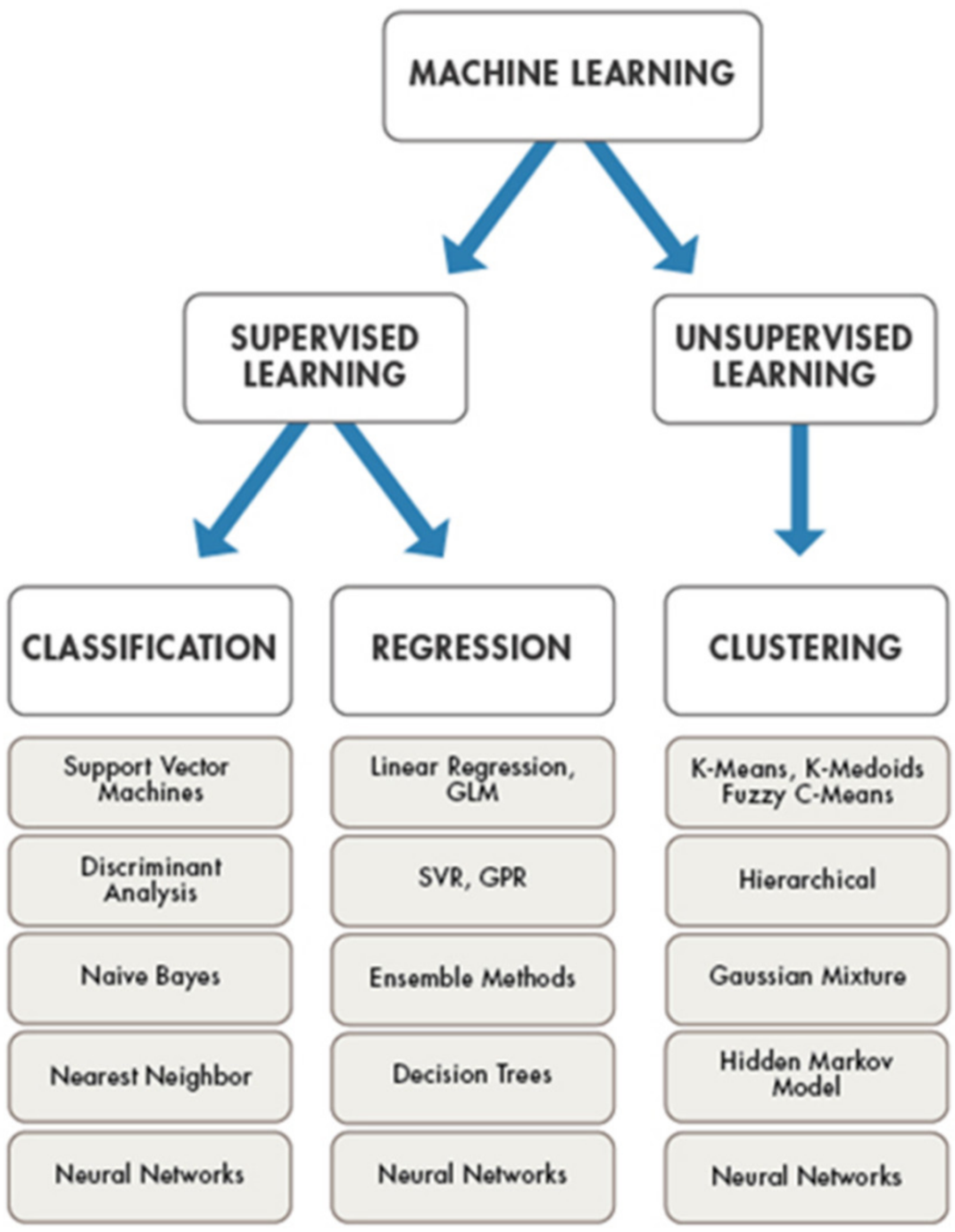
Figure 1 shows a simplified classification diagram of machine learning algorithms including generalized linear model (GLM), support Vector Regression (SVR) and gaussian process regression (GPR).
In manufacturing, SVM is the most commonly used algorithm in supervised machine learning. Machine learning is a powerful tool and its value will increase in the coming days. Machine learning is finding applications in many fields; some commercial fields are face recognition, image processing, manufacturing, and medical areas.
Machine learning (ML) can be applied in the domains of all industries. Machine learning approaches are implemented in procedural compliance, documentation of processes and orientation, and risk and quality frameworks of the manufacturing industry. The ability of machine learning to predict failure before it occurs is a useful feature, and some manufacturing firms are already using it in production to minimize financial losses and reduce risk [43].
Prediction   error % = | Expt .   Value     Pred .   Value | Expt .   Value × 100
Prediction error which is shown in Equation (1) is a principal tool that processes the performance of a training model, in which the estimation model is confirmed with new data that were not used earlier to examine the model. This tool was used to define the error percentage of the training models. Additionally, Root Mean Square Error (RMSE) is a common method of measuring a model’s error in numerical information estimation. It is described formally as follows Equation (2):
R M S E = 1 N i = 1 N p i q i 2
where N is the complete training data, pi is the estimation of the deliberate information, and qi is the actual value. RMSE method has been applied to evaluate the prediction performance of this study.

3.1. Artificial Neural Network

Neural network (NN) technology is an important branch of statistical machine learning and has been frequently used in various kinds of forecasting tasks. Artificial neural networks (ANNs) are the most widely used AI models; they simulate the ability of brain neurons to process information. The use of ANNs to solve forecasting problems has recently attracted considerable research attention because they substantially outperform previously implemented techniques for forecasting based on nonlinear input variables. ANNs are extremely good at modeling the nonlinearities in data in many fields and have theoretically proven capability to approximate any complex function with arbitrary precision. ANNs are inspired by natural neural networks and are computer programs developed to obtain information in a manner similar to the human brain. Artificial intelligence is a combination of neural networks that were developed based on research on cognitive talent and machinery design. ANN is a tool commonly used for prediction and categorization in data processing inspired by the attributes of biological neuron systems that learn by experience. It has many features that make it attractive for problems such as pricing options, with the capability of developing nonlinear model relationships that do not depend on the restrictive assumptions implied in the parametric approach, or on the specification of the theory that connects the prices of underlying assets to the prices of options. The implementation of an ANN model is considered successful when it has the ability to learn from the provided data and use the data in a new way [44,45,46,47,48].
The ANN’s model strength lies in the relationship between the input and output variables, which can be complex and difficult to get from mathematical formulation [49]. Staub et al. explored the features that make ANN the most important tool to solve complex nonlinear problems [50]. ANNs modify their own values and are able to adapt to the exact solution of the problem. During the training process, ANNs are able to create the desired response. In the past, expert systems and neural networks were used extensively for electricity load forecasting. In the past, professional models and neural networks were commonly used to predict power loads. In recent times, they are also being used to estimate long-term energy demand, taking into account macroeconomic variables. Neural networks are used to model the energy consumption of appliances, lighting, and space cooling in the Canadian residential sector [51]. Kandananond applied artificial neural networks to forecast electricity demand in Thailand [44]. In this study, an ANN prediction model is trained for each component using the Levenberg–Marquardt algorithm, which shows stable and fast convergence. 
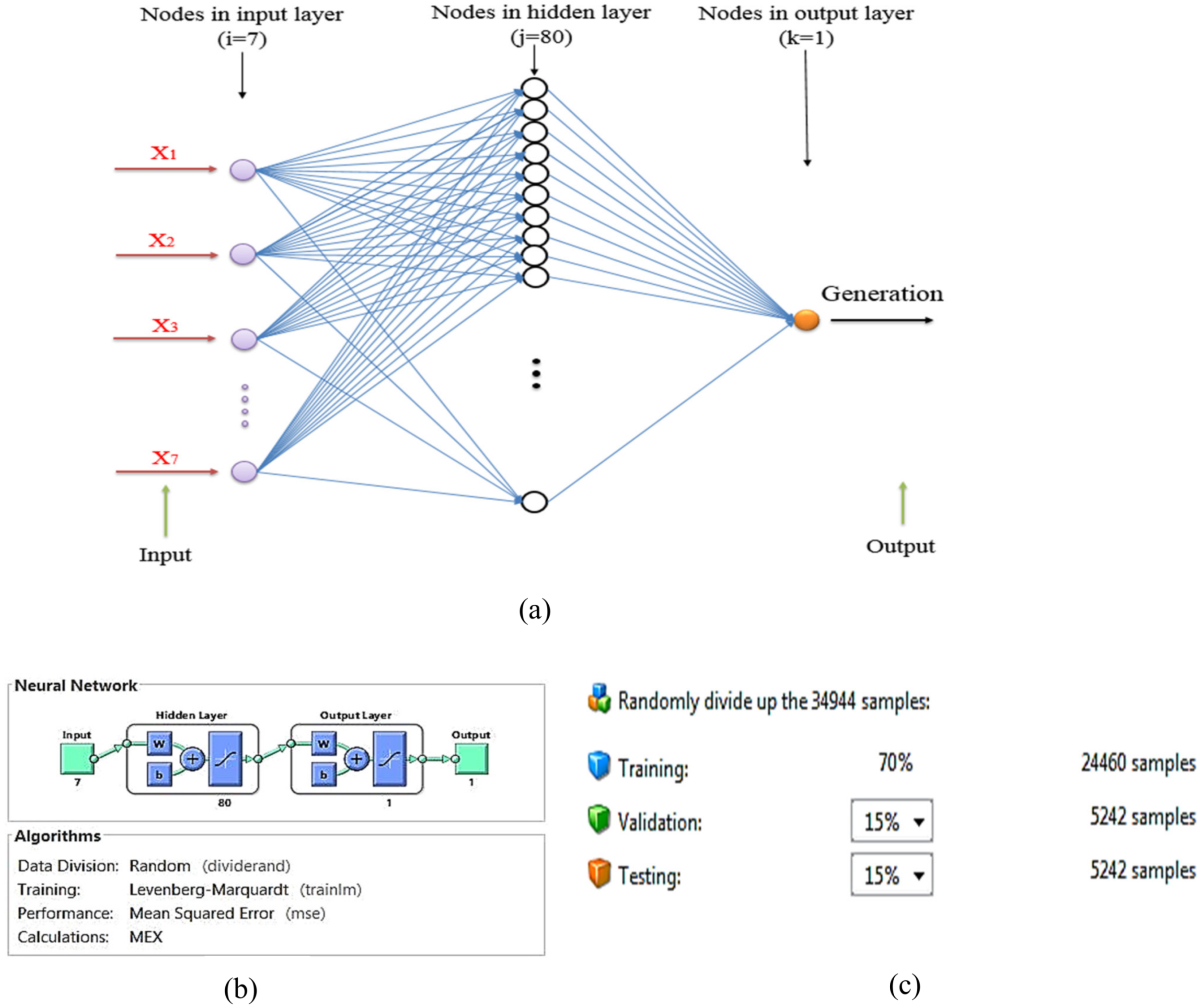
Figure 2 shows the design of this ANN: three layers with full connection and seven input nodes are logged into the input layer to describe one output. Input nodes (X) include time, temperature, humidity, solar irradiation, population, GNI, and electricity price per kWh. The output of this design is electricity generation.
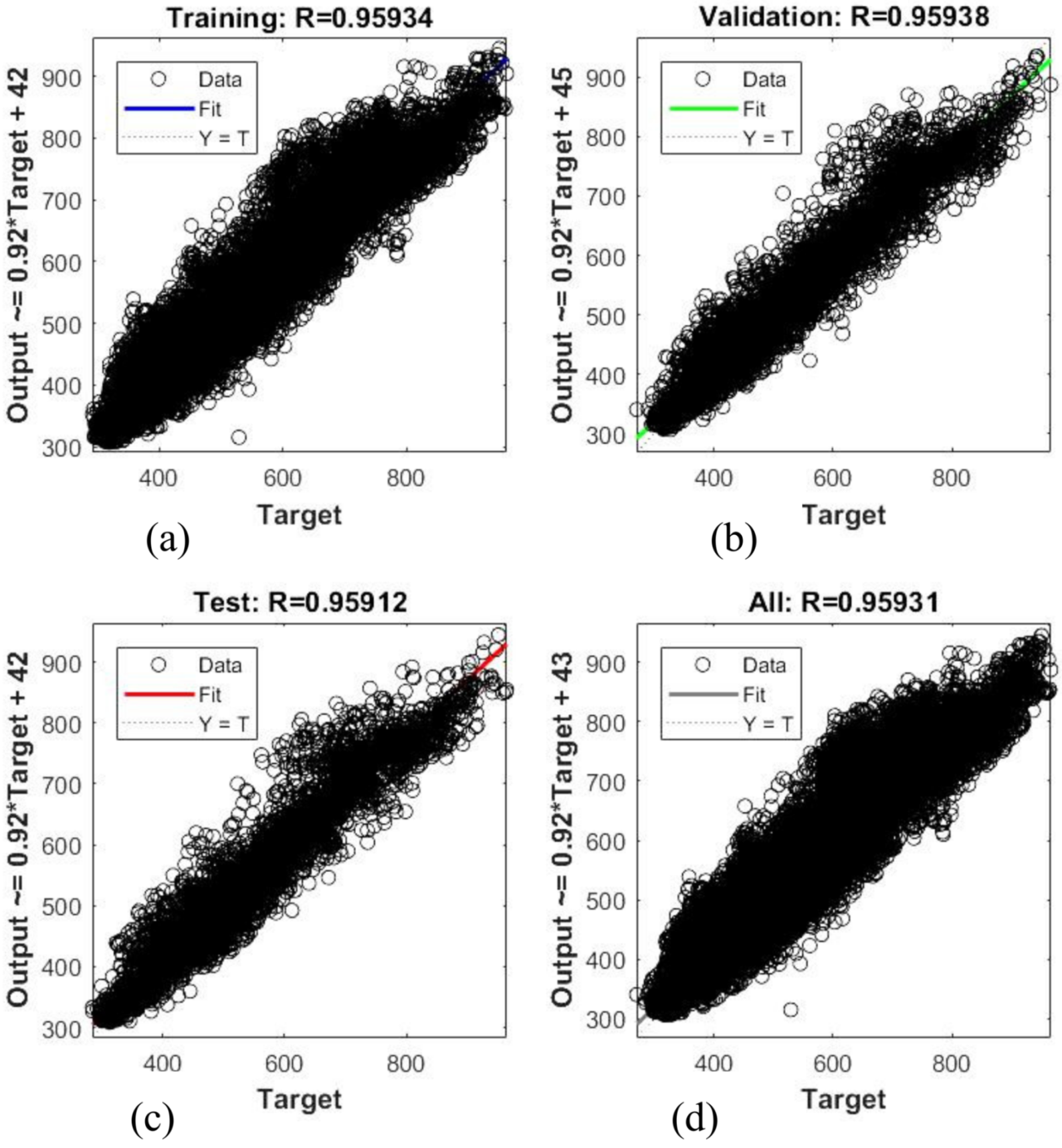
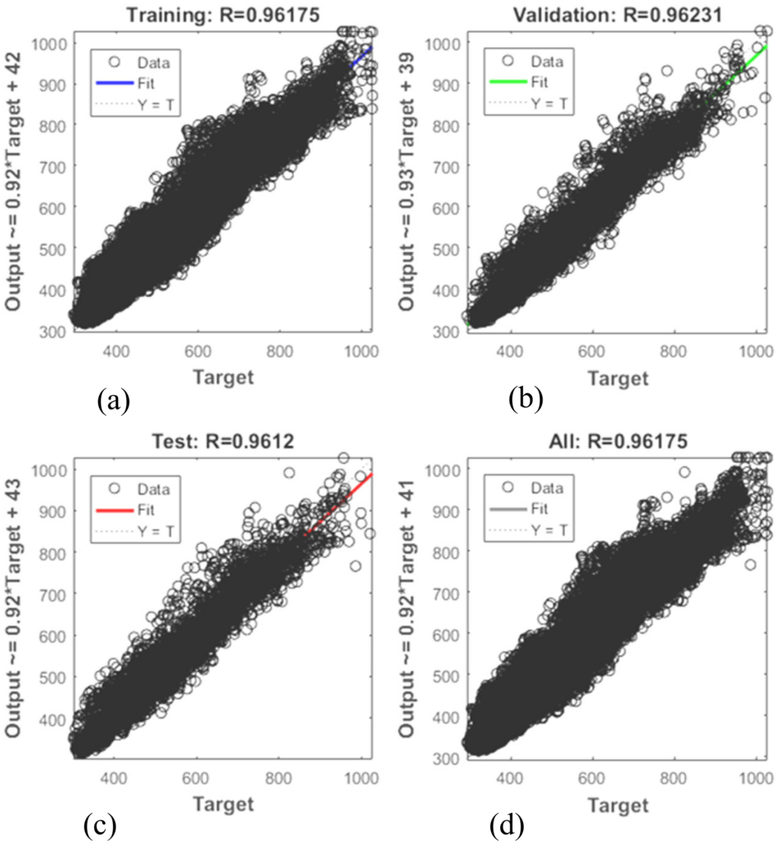
Figure 3 and Figure 4 show the schemes of long-term record regressions for all datasets for 2016 and 2017, respectively. This figures explain the correlation between the target (experimental data) and the ANN model output. The dashed line in each figure represents the targeted values. The best-fit linear regression line between the outputs and targets is represented by a solid line.
The regression coefficient of both ANN models is very close to one, which is satisfactory. The average error of the training model for 2016 and 2017 is 5.57% and 5.28%, respectively. Additionally, Figure 5 and Figure 6 show outlines of short-term record regressions for all datasets for 2016 and 2017, respectively. Similarly, the regression coefficient of ANN models for short-term analysis is near one, which is desired. The average prediction error of short-term analysis for 2016 and 2017 is 0.97% and 1.67%, respectively.

3.2. Adaptive Neural Fuzzy Inference System

ANFIS stands for adaptive neuro-fuzzy inference system. The ANFIS toolbox feature forms a fuzzy inference system whose membership structure parameters are calibrated (adjusted) either using a backpropagation method or in combination with a least-squares-type method. This adjustment allows the fuzzy systems to learn from the data they are modeling. Neuro-adaptive training strategies provide a mechanism for fuzzy modeling to learn details about a dataset. The Mamdani fuzzy inference system’s basic structure is a framework that maps input features to input membership functions, input membership features to rules, rules to a series of output features, output characteristics to output membership features, and output membership functions to a single-valued output or a decision associated with the output. Such a system uses fixed membership functions that are chosen arbitrarily and a rule structure that is essentially predetermined by the user’s interpretation of the characteristics of the variables in the model. The fuzzy inference style utilized in this paper contains seven inputs, three membership functions for every input. The Sugeno fuzzy design is made consistent with two IF rules, which are established as follows [52]. The ANFIS utilized in this investigation was settled with MATLAB. 
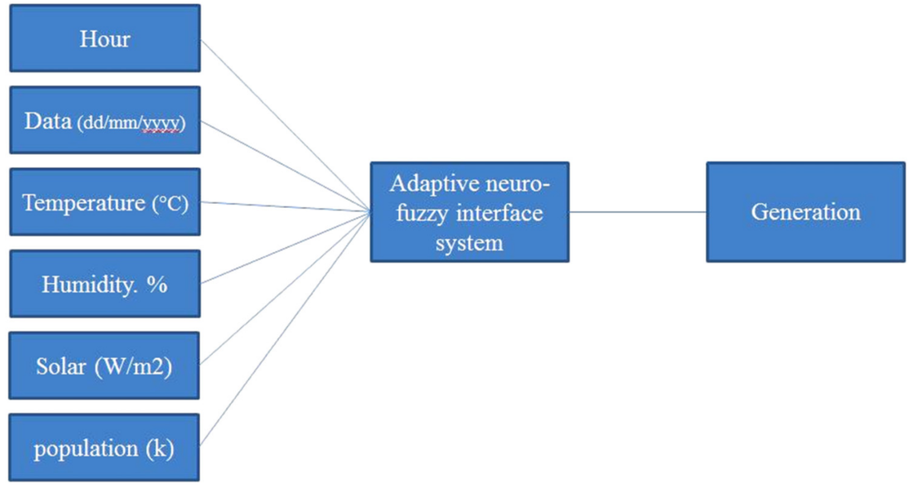
Figure 7 demonstrates the developed ANFIS model.
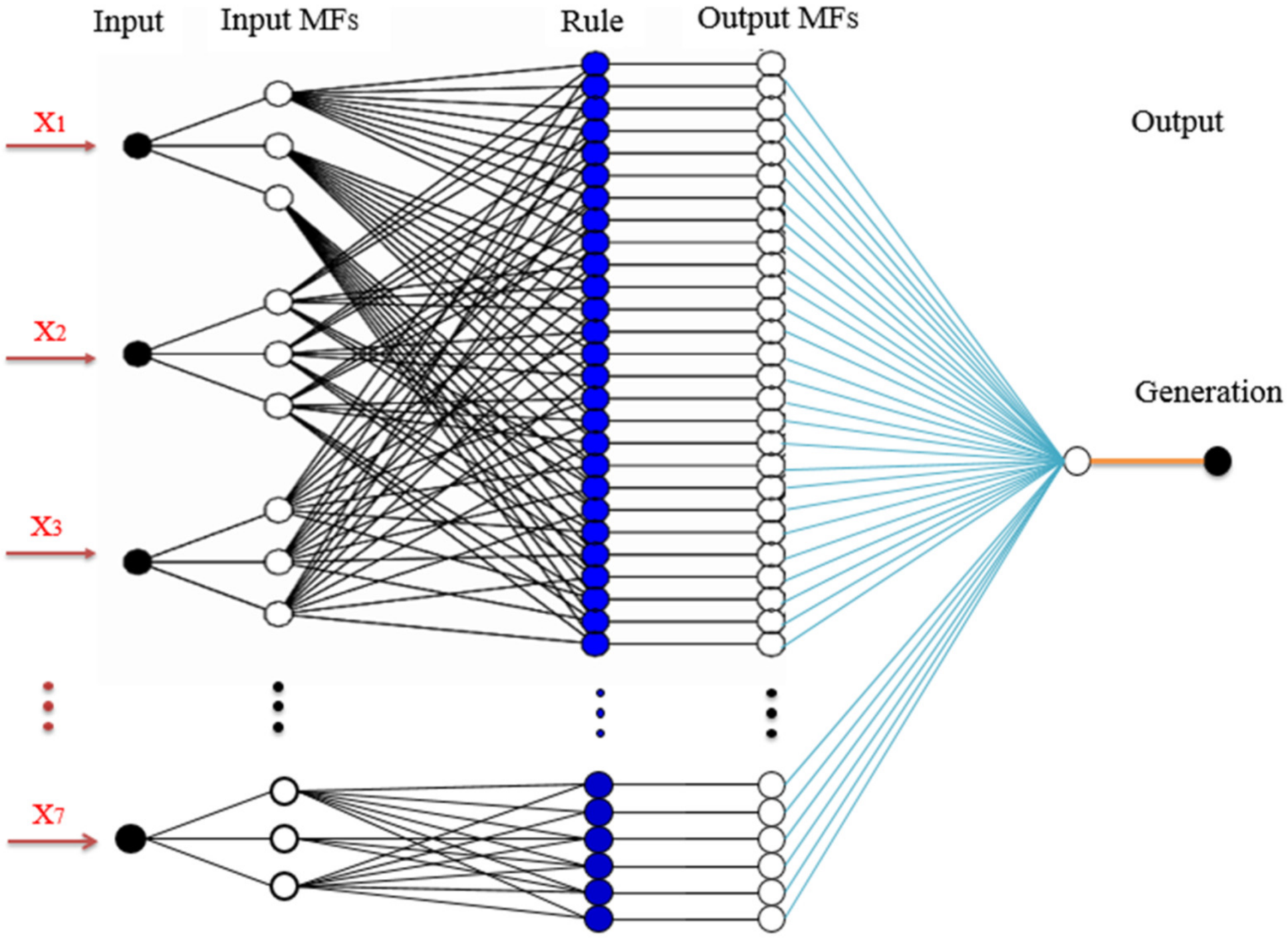
The planned ANFIS design for the generation is shown in Figure 8. It includes seven nodes in the input layer, 100 nodes in the hidden layer, and one node (generation) in the output layer.
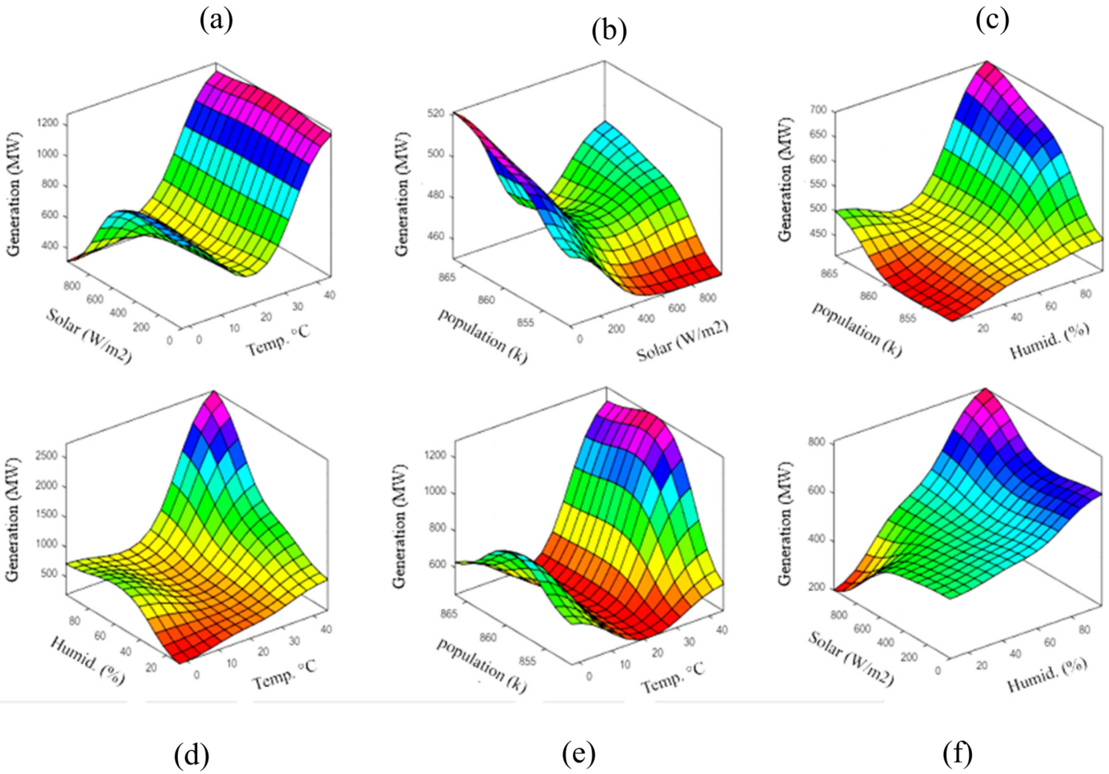
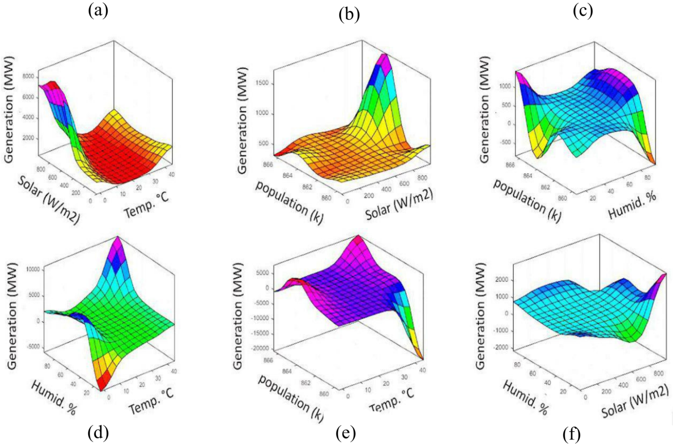
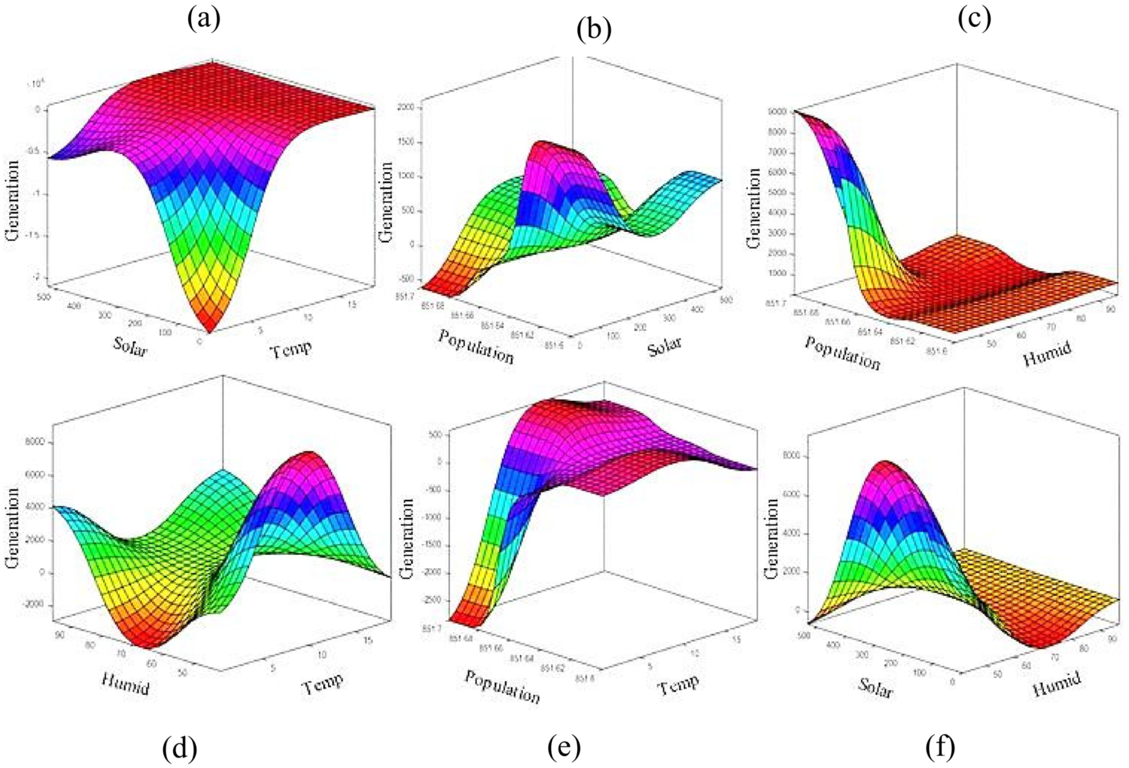
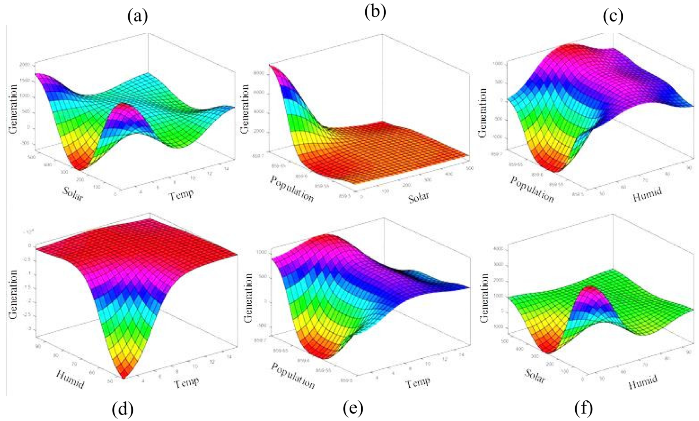
 Figure 9 and Figure 10 show the contour and 3D graphs of generation values with different input parameters for long-term analysis. Figure 11 and Figure 12 show the contour and 3D graphs of generation values for short-term analysis. The results of the graphs show that generation increases with increased humidity, solar irradiation, and temperature. On the other hand, generation decreases with decreased humidity and population.
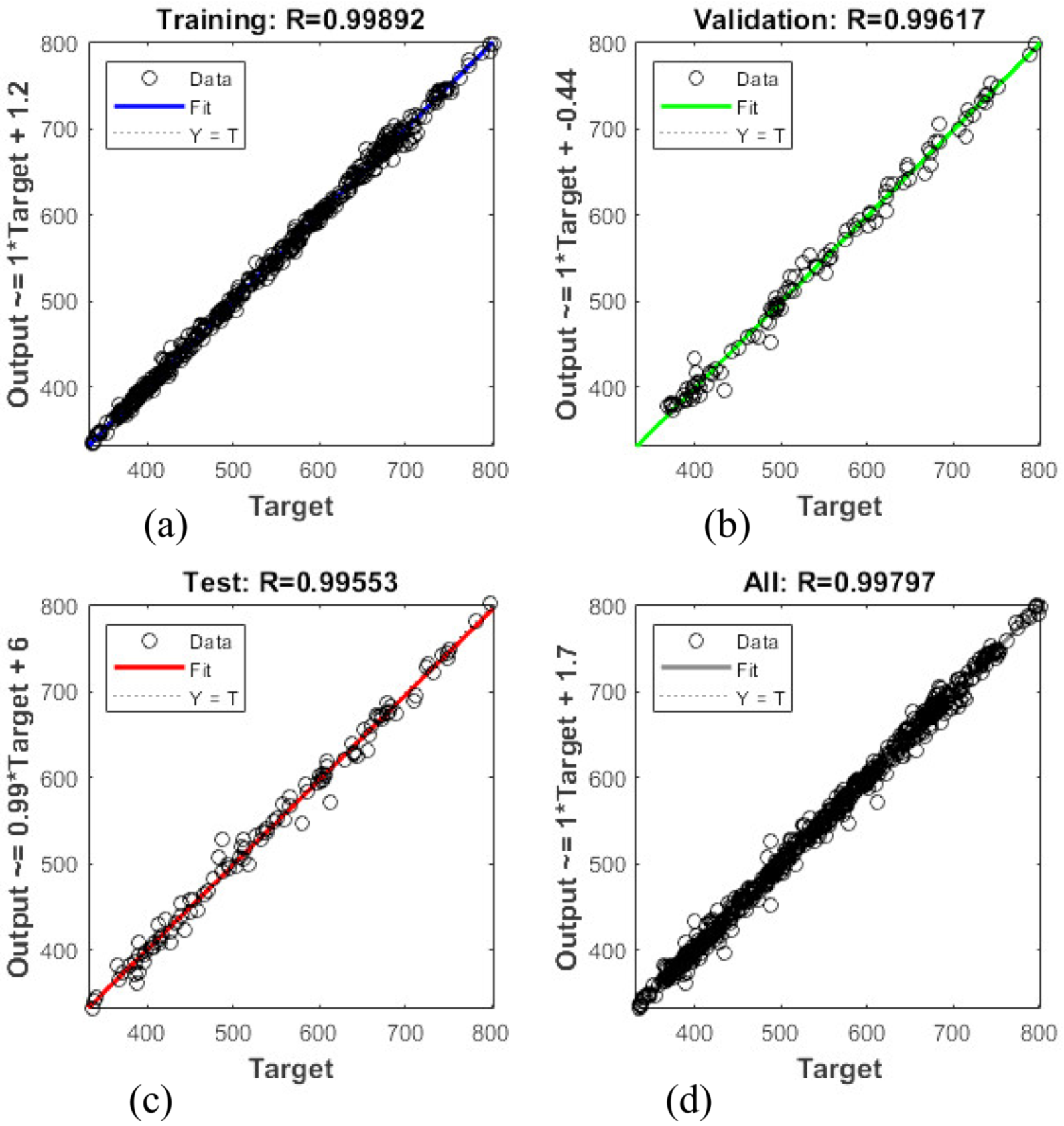
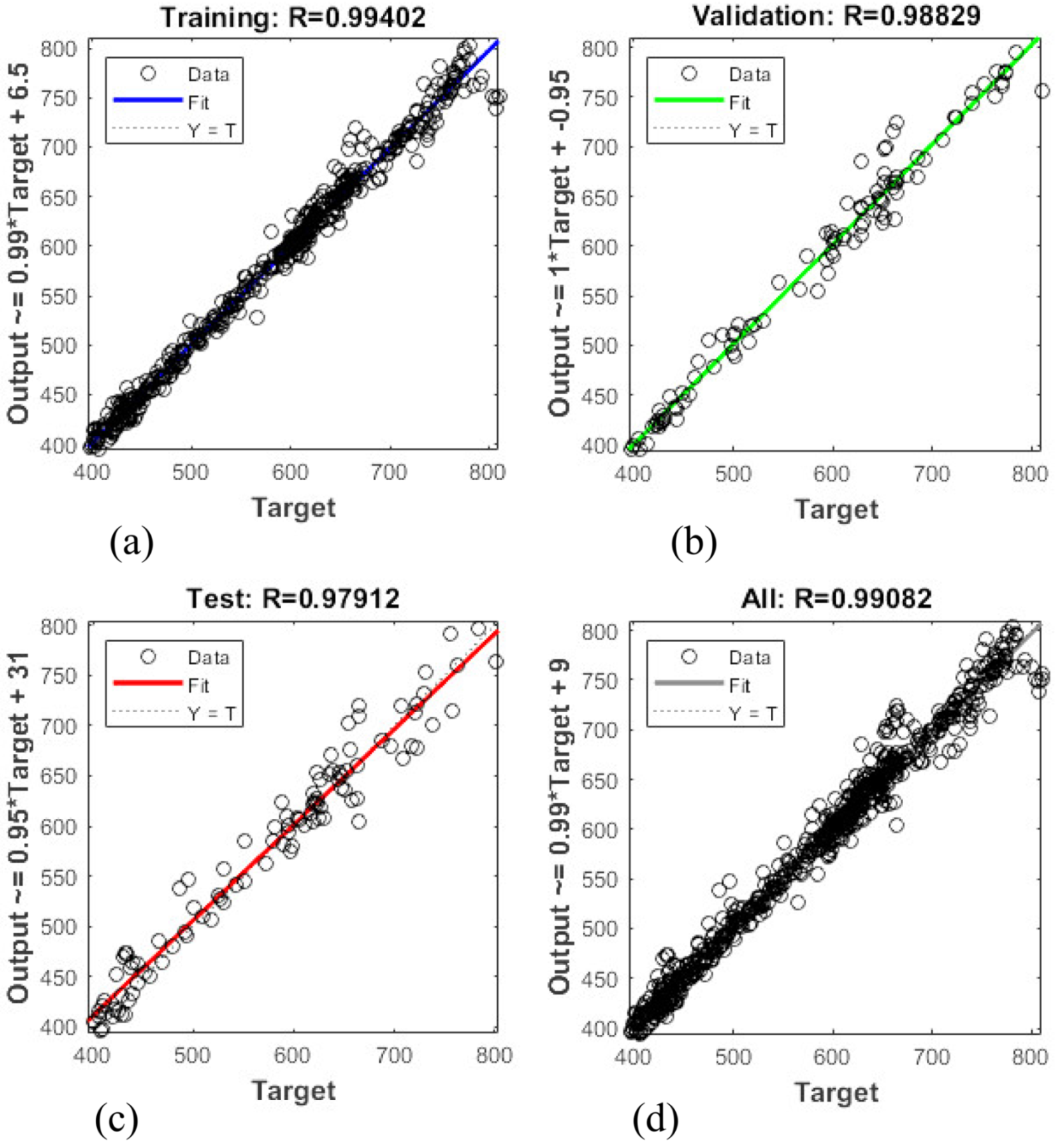
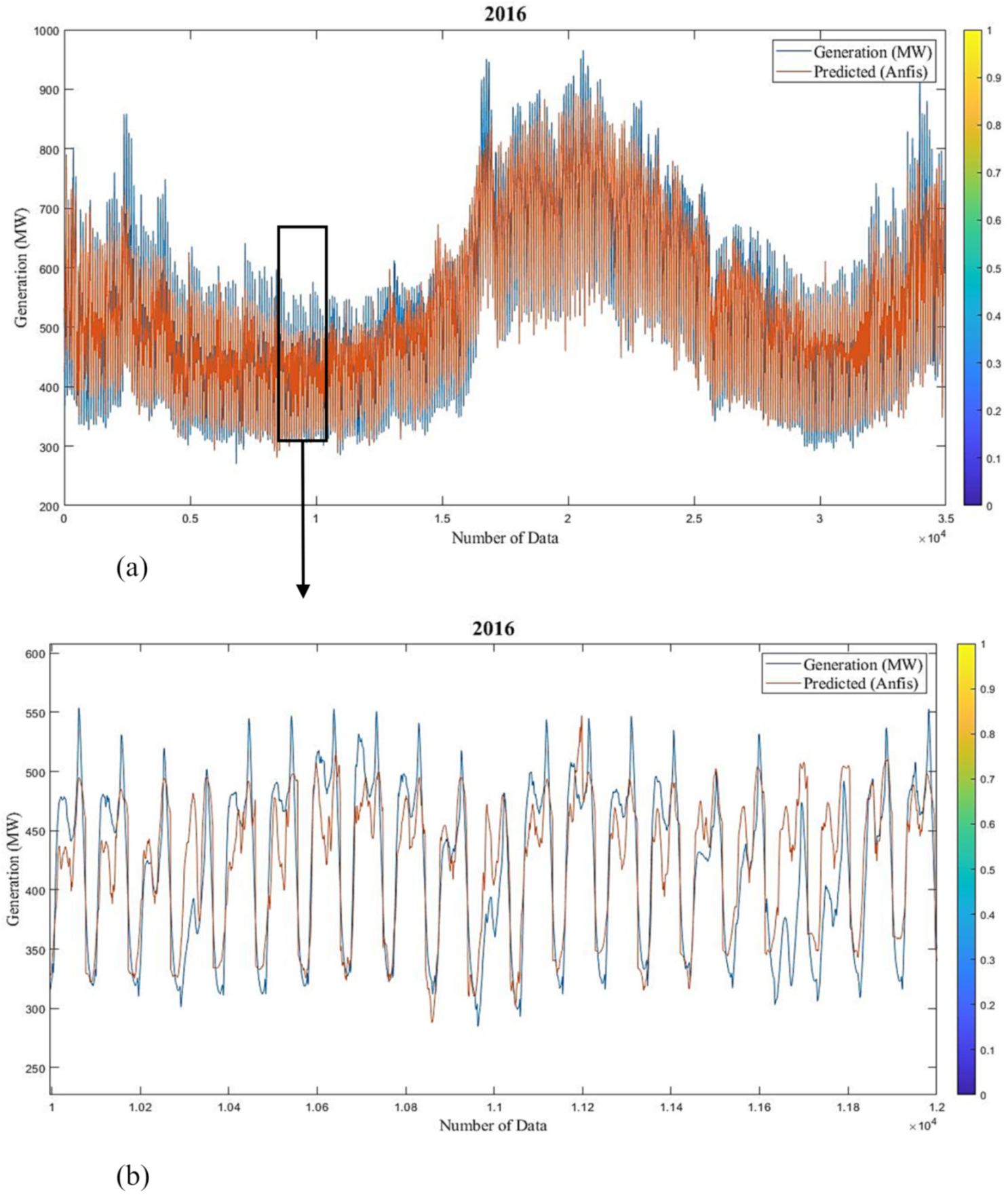
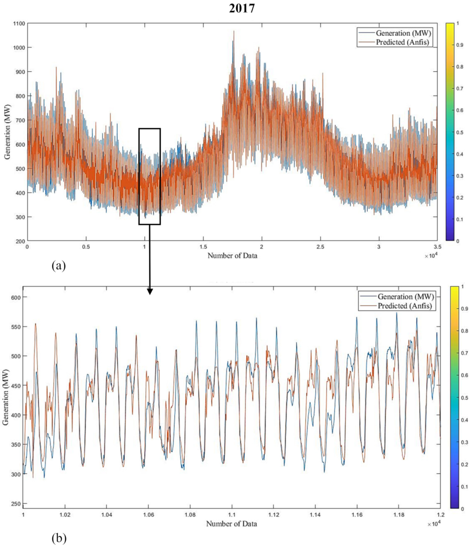
 Figure 13 and Figure 14 show graphs of estimated versus actual values of long-term study for 2016 and 2017, respectively.
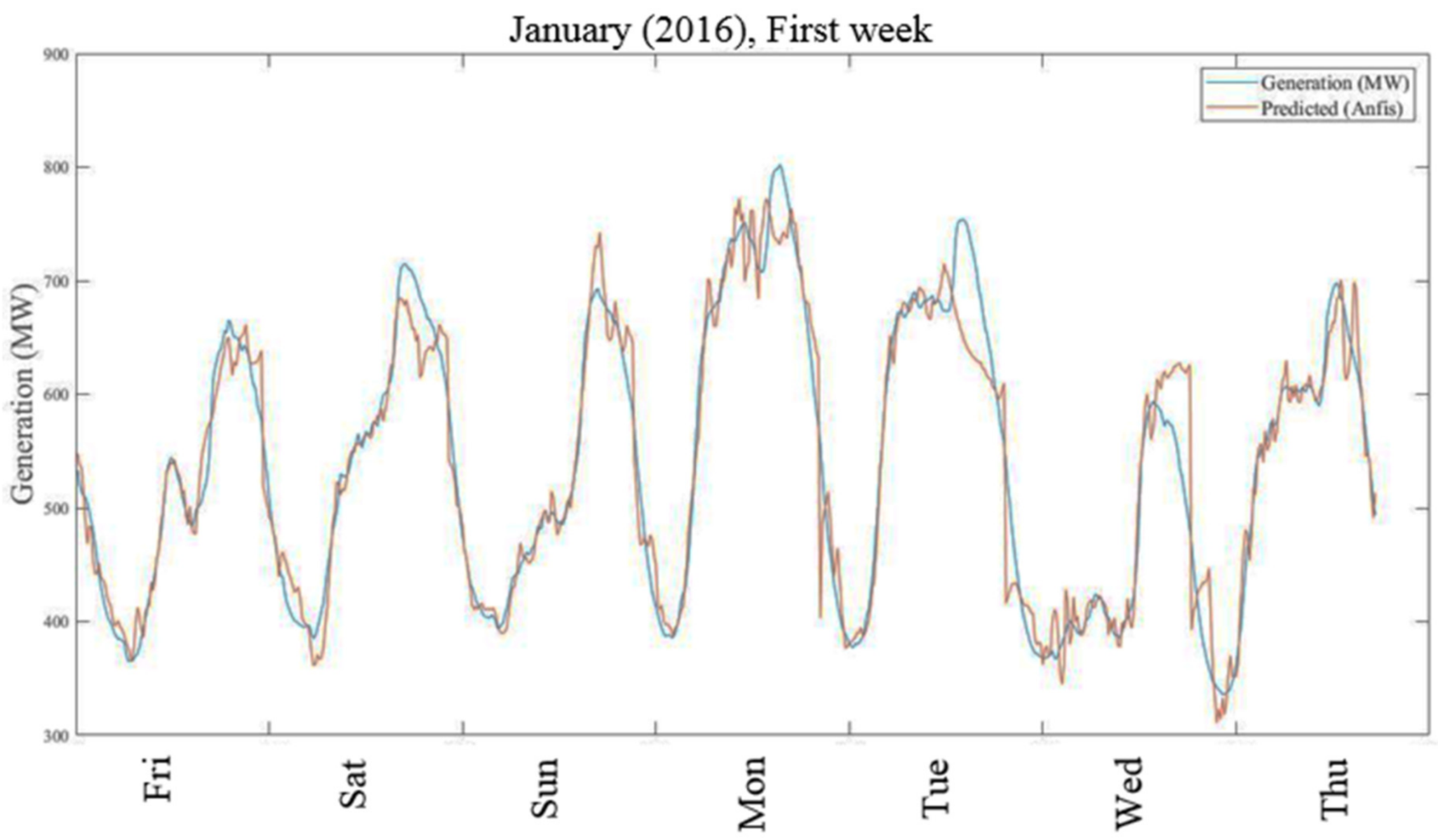
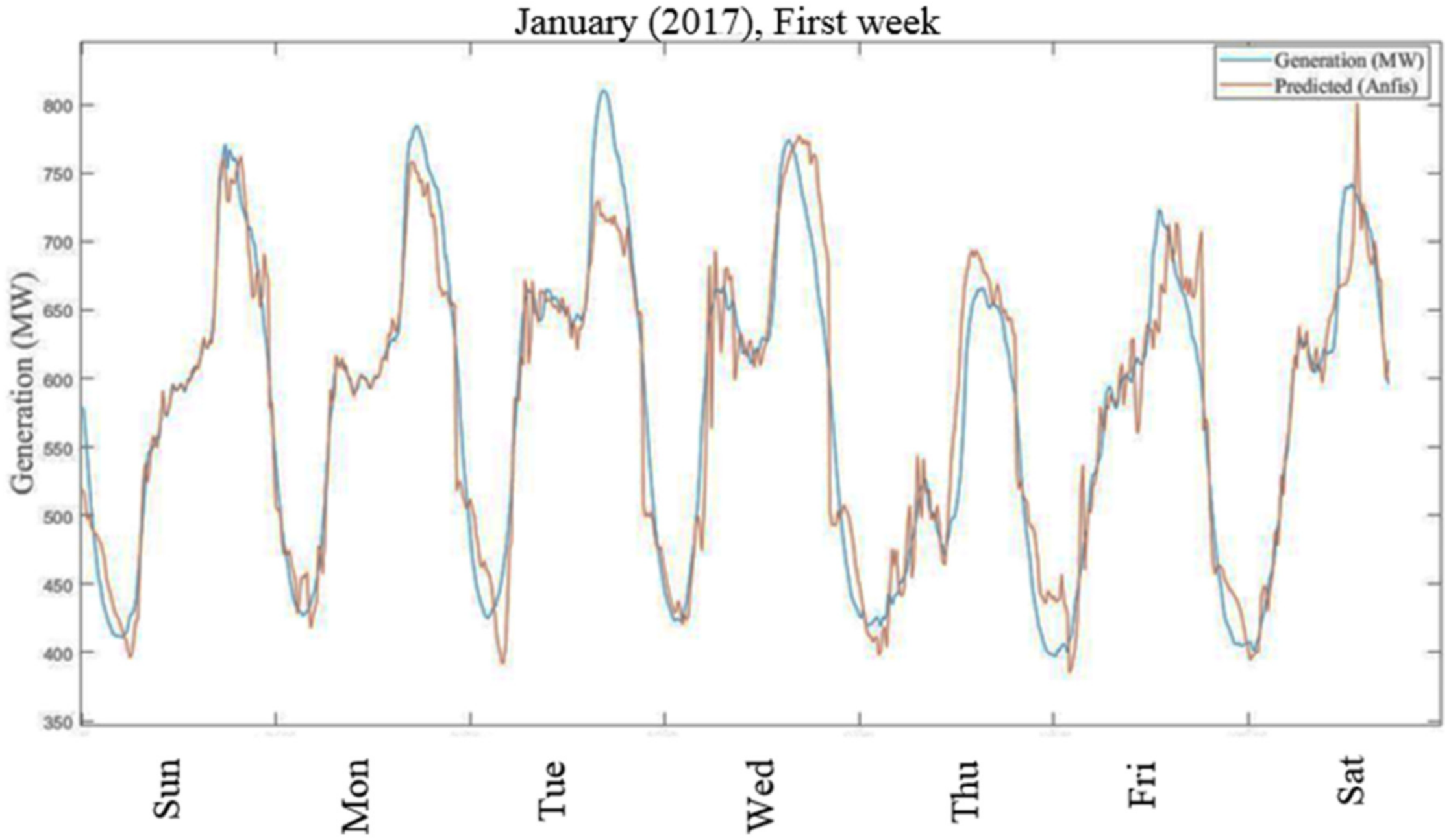
 Figure 15 and Figure 16 show graphs of predicted versus actual values of short-term study for 2016 and 2017, respectively. Results show that estimated values are in good agreement with the actual responses. The average prediction errors of the long- and short-term ANFIS training models for 2016 and 2017 are 7.69% and 6.11%, and 3.75% and 3.89%, respectively.

3.3. Multiple Linear Regression

Regression analysis is one of the most commonly used traditional forecasting/prediction techniques to identify causality between dependent and independent (explanatory) variables. The association between dependent and predictor variables is formulated as a linear model in Equation (3):
Y = β_0 + ∑β_i X_i + ε_i
In this formula, β0–βp are the regression coefficients to be estimated according to observations. To avoid multicollinearity problems, correlations between predictors should be controlled (the correlation coefficient of the explanatory variables should not exceed 0.7) [53]. The last term in the formula, ε, denotes the random error and is referred to as the residual to check the overall significance of the model and each regression coefficient [54]. The error term is independently and normally distributed, with a mean of zero and a constant variance of σ2 [55]. Regression models describe the relationships between output values and one or more input values. A multiple regression model is a parametric model. There are many statistical and machine learning methods to generate results, such as linear, generalized, and nonlinear regression models, containing mixed effects and stepwise models. The relationship between the numeric predictor and the continuous target is approximated by simple linear regression by using a straight line. The relationship between a set of p > 1 predictors and a single continuous target approximates multiple regression modeling using a P-dimensional plane [56]. One of the main objectives of regression modeling is to select the best suitable regression that can develop an accurate response variable. Regression trees (RTs) and ANNs are ambitious techniques for modeling regression problems. Multiple linear regression (MLR) is a classic technique that delivers many benefits: clarity, interpretability, the potential to be modified over parametric transformations, and reasoning, assuming the normality hypothesis, homoscedasticity, and inter-correlation between the error ε and the predictor variables.
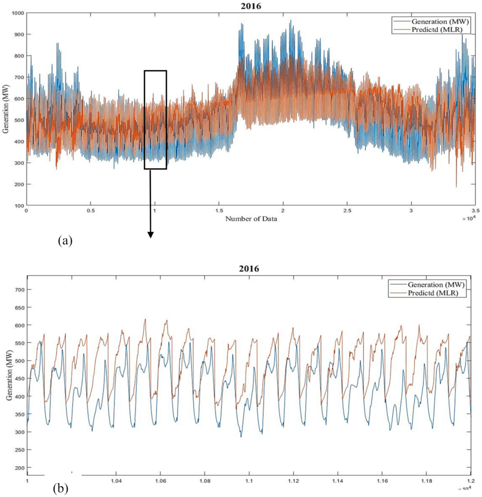
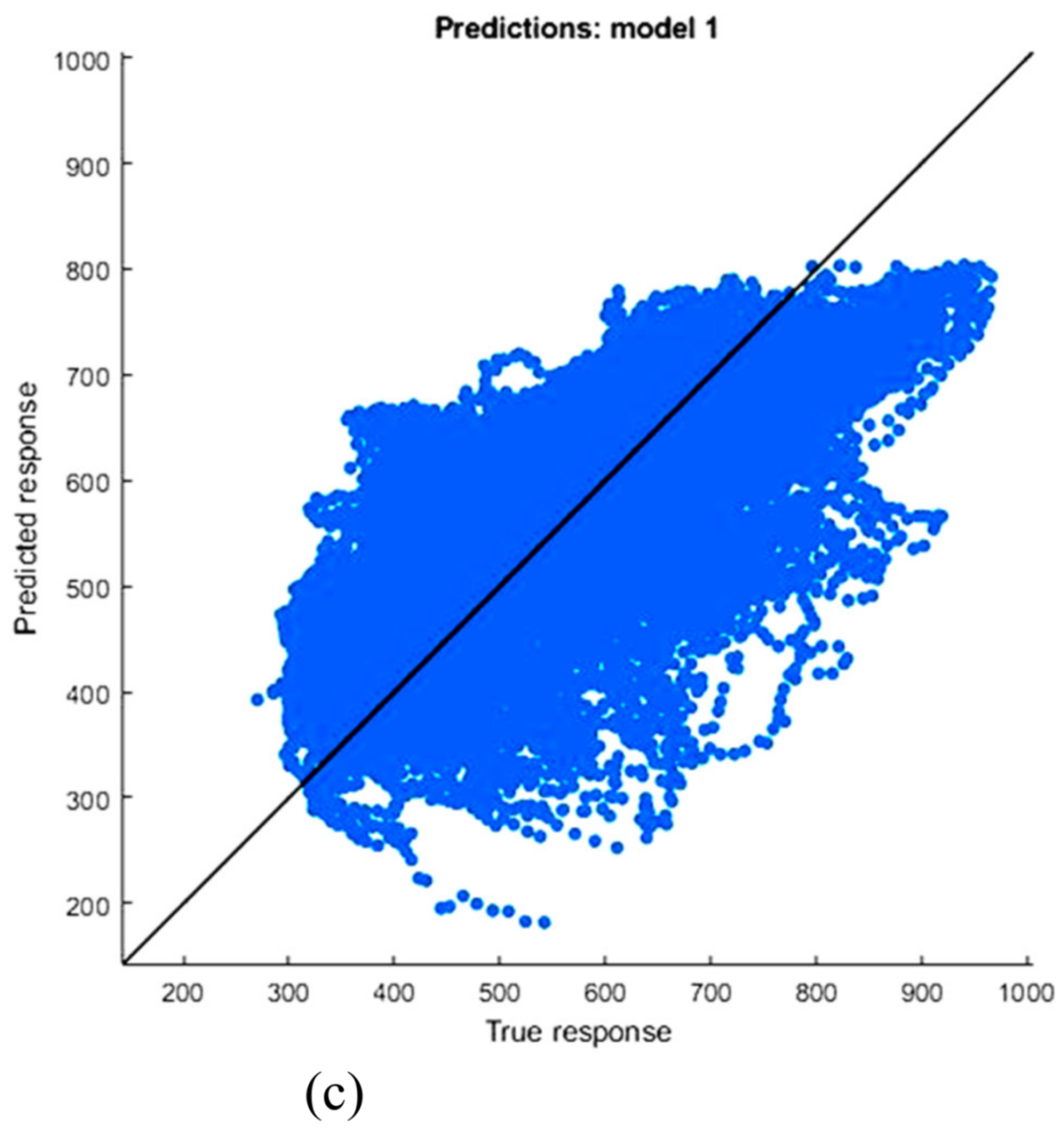
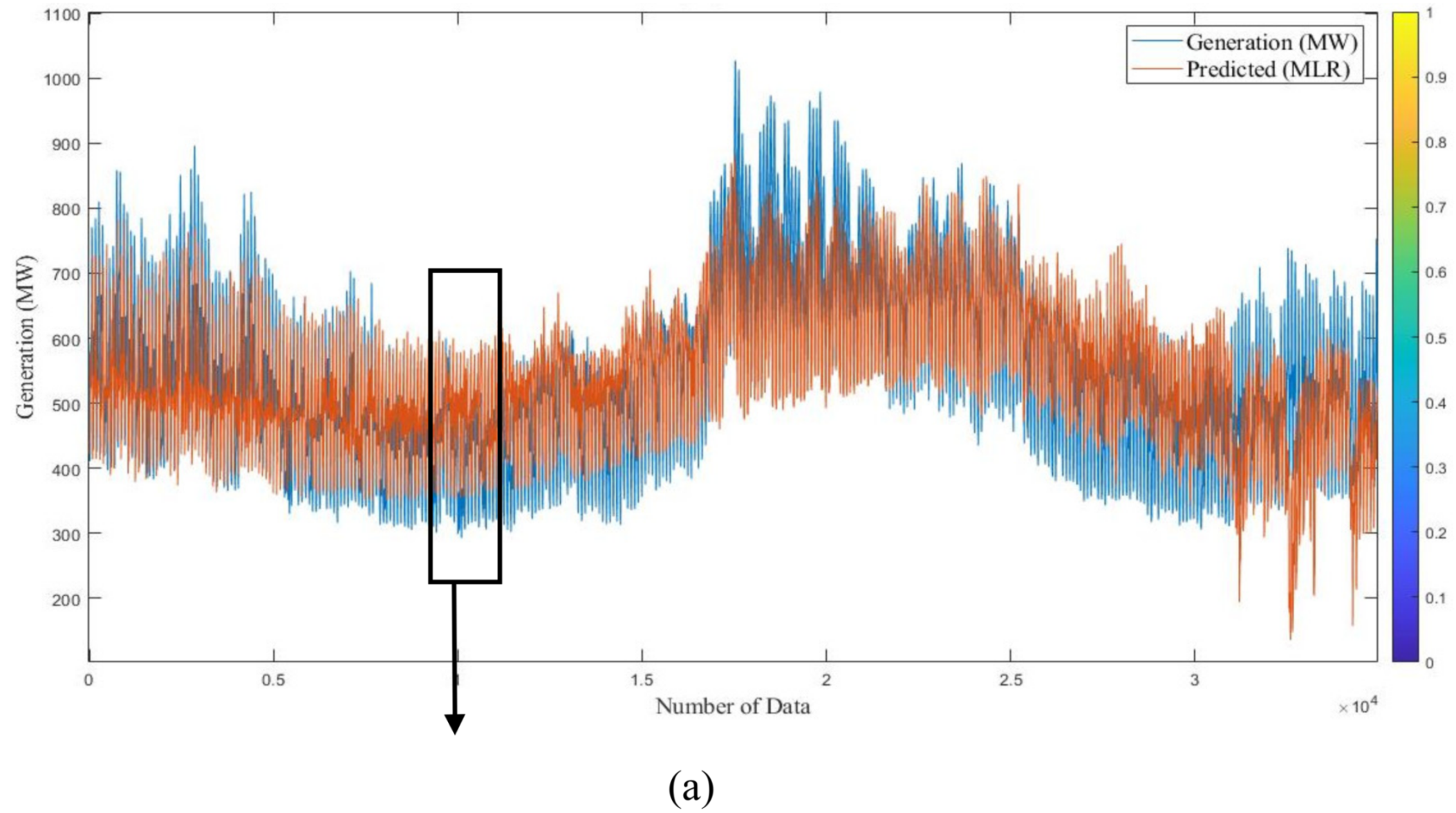
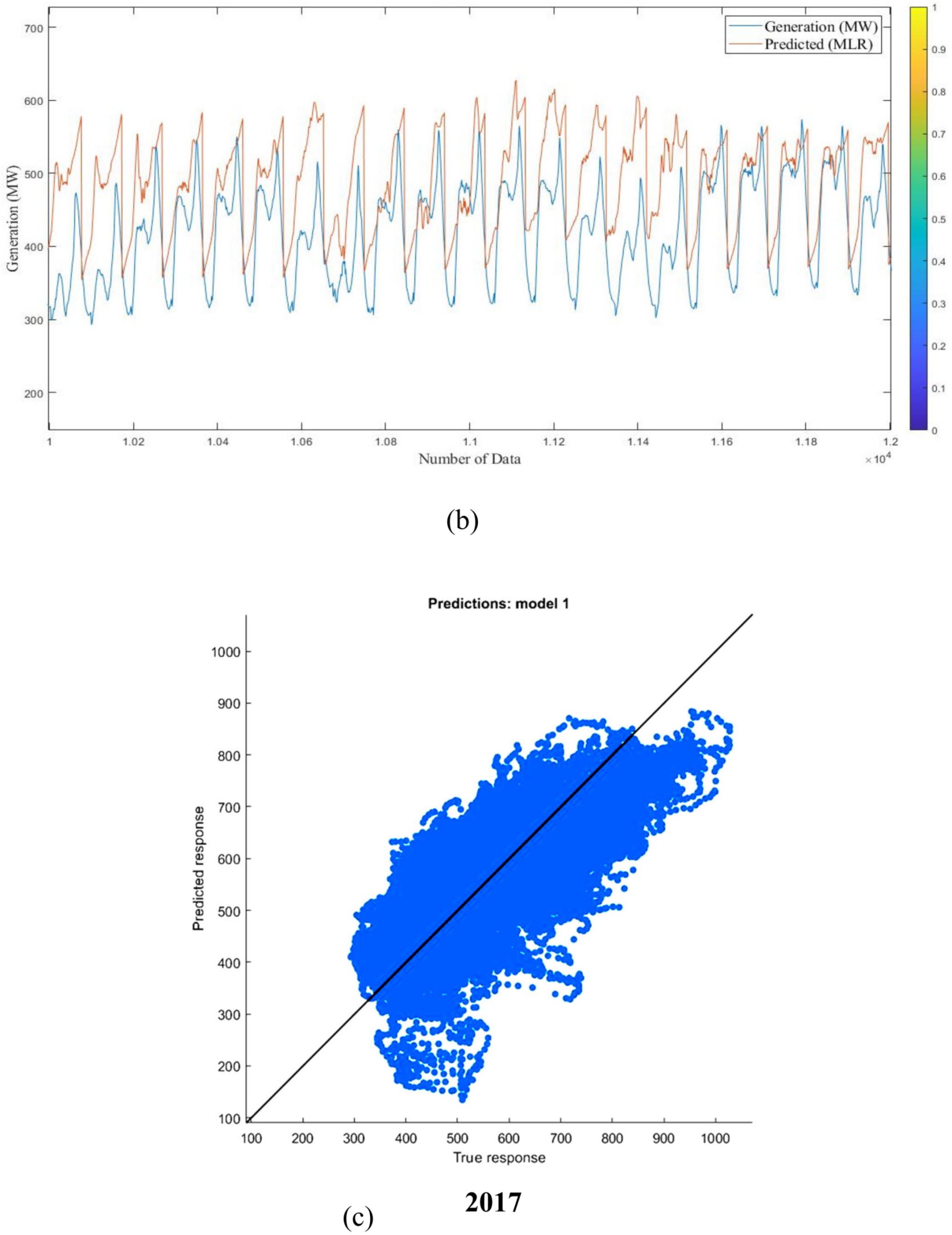
 Figure 17 and Figure 18 show outcomes of MLR numerical investigation of estimated versus actual responses of long-term examination, with scaled coefficients, where the solid line symbolizes the fitting line. Figure 19 and Figure 20 demonstrate the results of the MLR numerical study of predicted versus actual responses of short-term examination. The graphs show that estimated and actual data are not well matched. The average prediction errors of long-term and short-term MLR models for 2016 and 2017 are 15.18% and 13.4%, and 10.44% and 9.08%, respectively.

3.4. Support Vector Machine

Support vector machines are used in many machine learning tasks, such as pattern recognition, object classification, and time series prediction, including especially the forecasting of energy consumption. Support vector regression (SVR) is an SVN method specifically for regressions. SVMs are based on the principle of structural risk minimization. The SVM constructs one or more hyperplanes in a high dimensional space. The objective of SVR is to minimize the probability that the model generated from the input dataset will make an error on an unseen data instance. The objective is achieved by finding a solution that best generalizes the training examples. Ma et al. (2018) applied SVM to predict building energy consumption in China [57]. The SVM algorithm was used to find a hyperplane with N-dimensional space (where N means number of characteristics) that clearly segregate the data points, and many possible hyperplanes were used to separate the two classes of data points. Finding a maximum margin plane is the main objective, for example, the utmost distance between data points of both classes. Overestimating the margin distance provides some support so that future classification of data points can be done with greater confidence [58,59].
Guo et al. and Fu used a support vector model for electricity load [60,61]. Kavaklioglu et al. derived electricity consumption as a function of socioeconomic indicators such as population, gross national product, and imports and exports [39]. This method was constructed on the structural possibility of minimization standard.
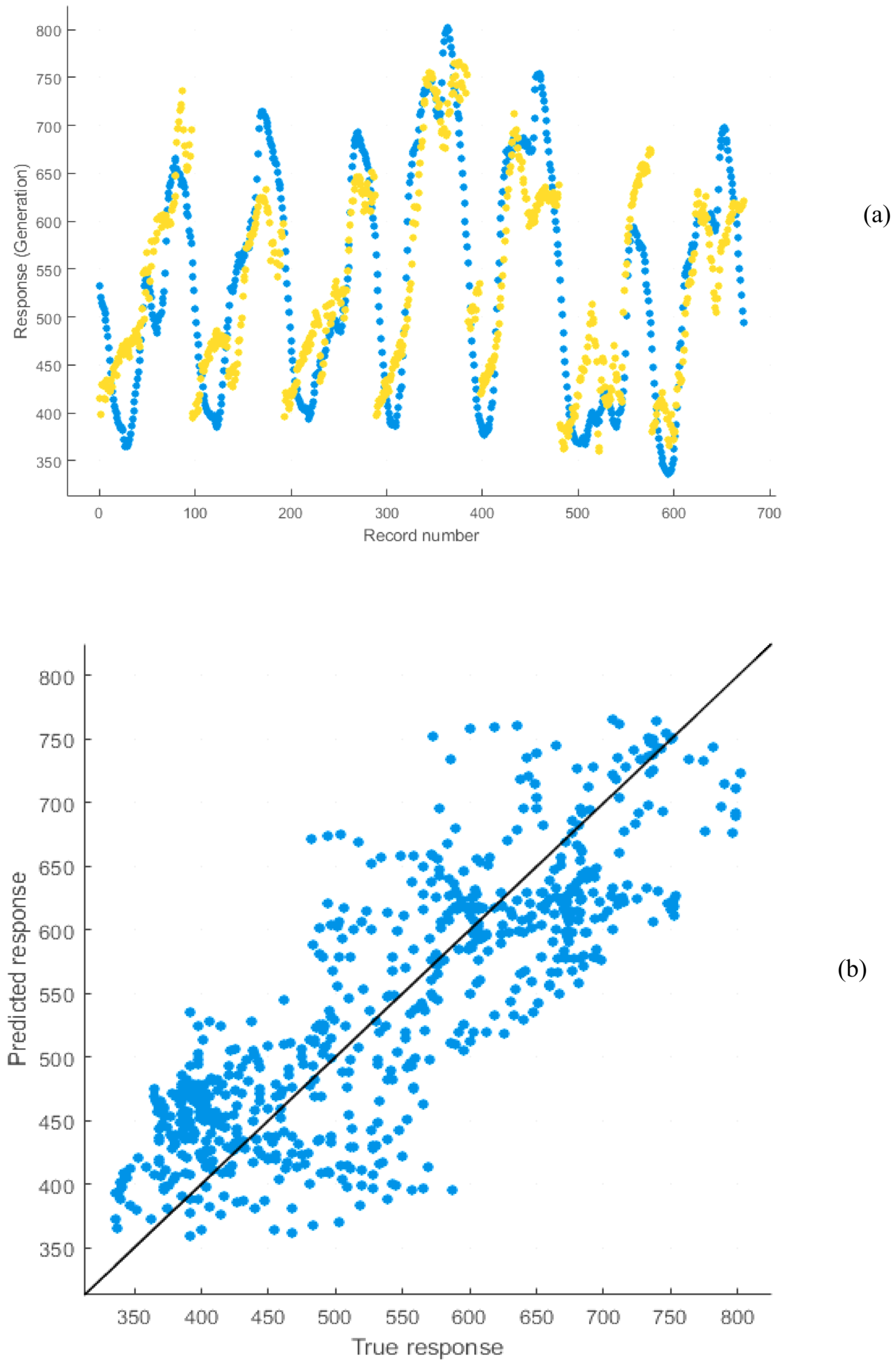
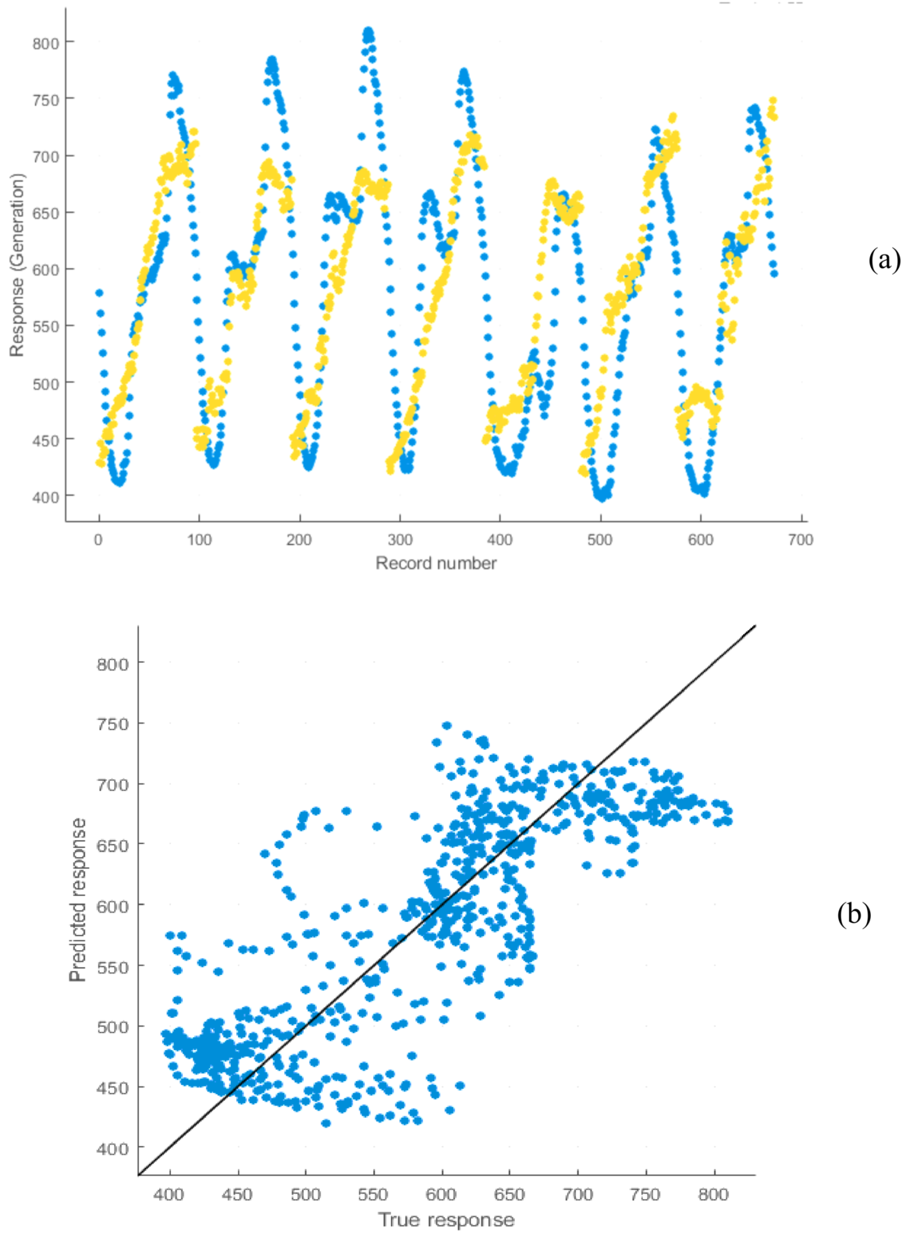
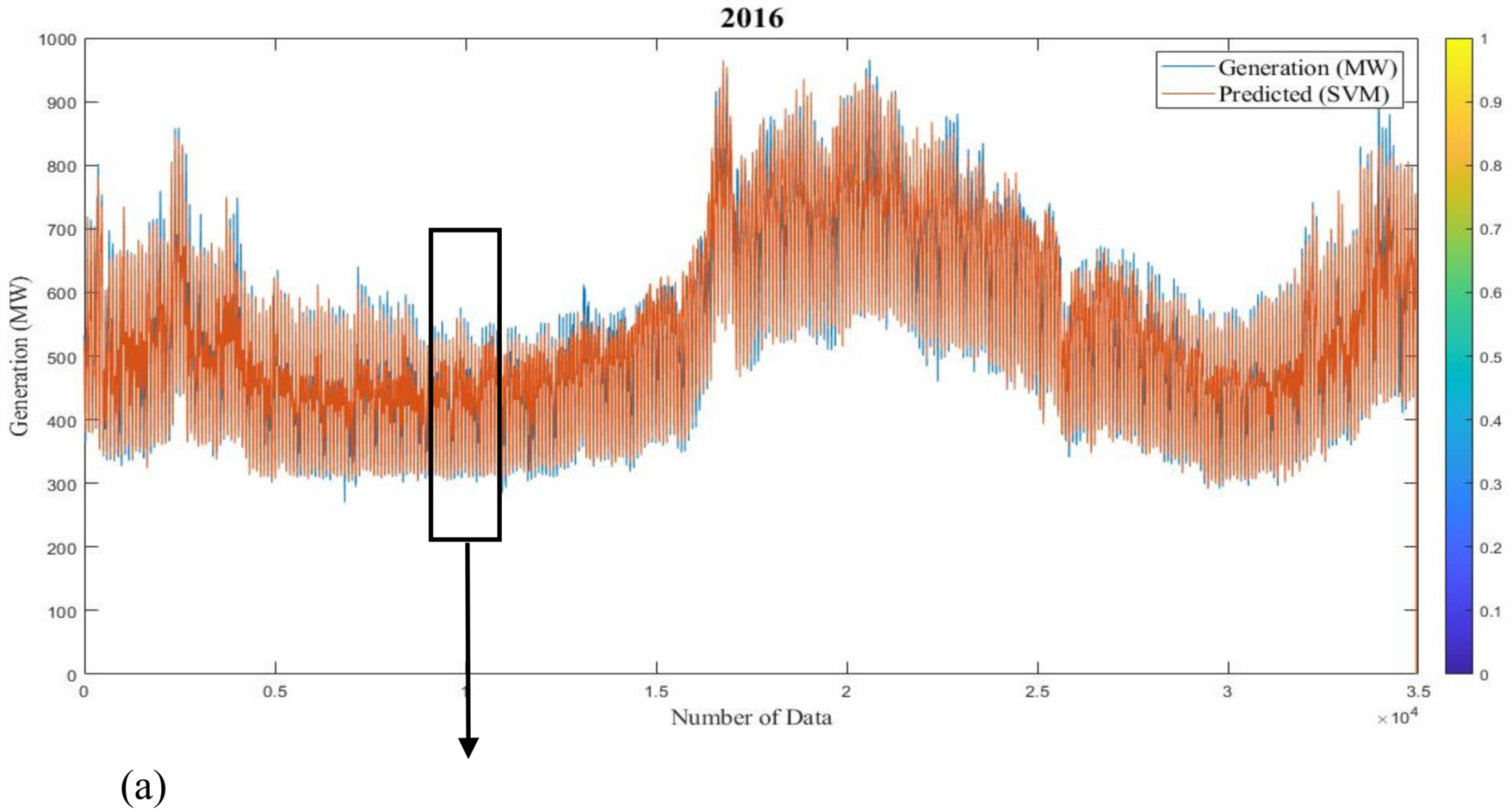
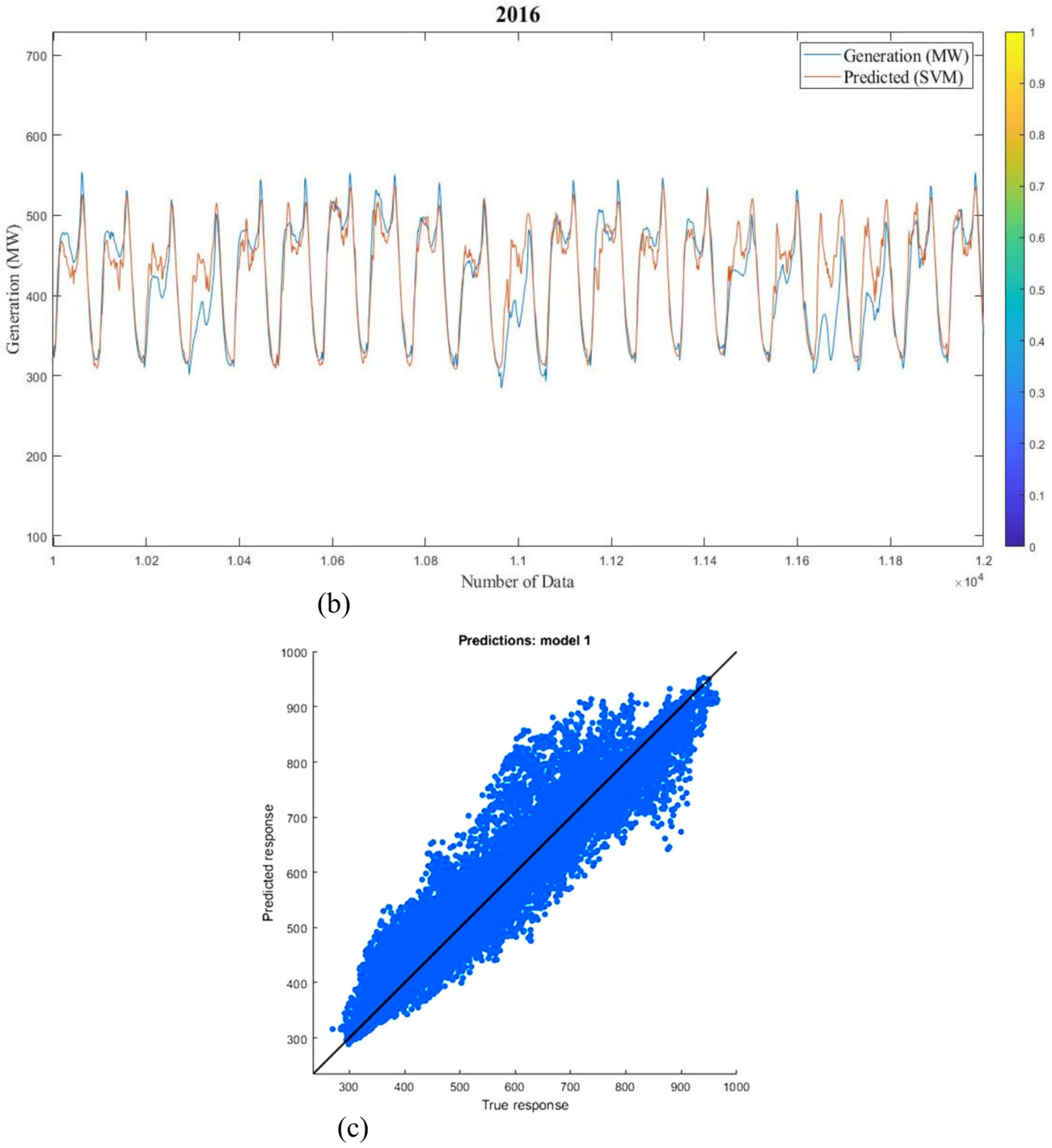
Figure 21 and 
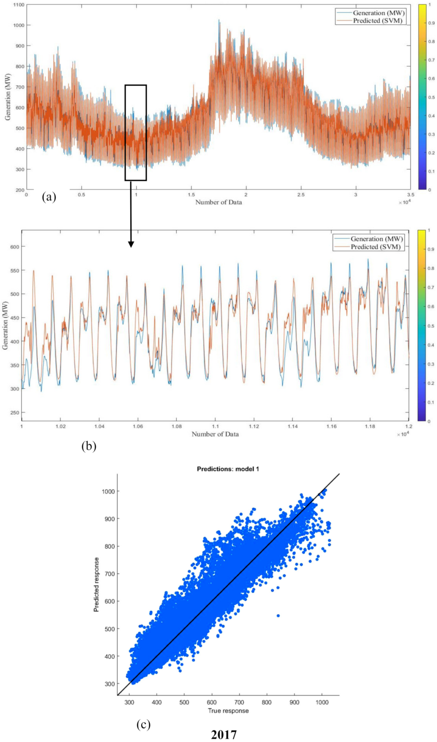
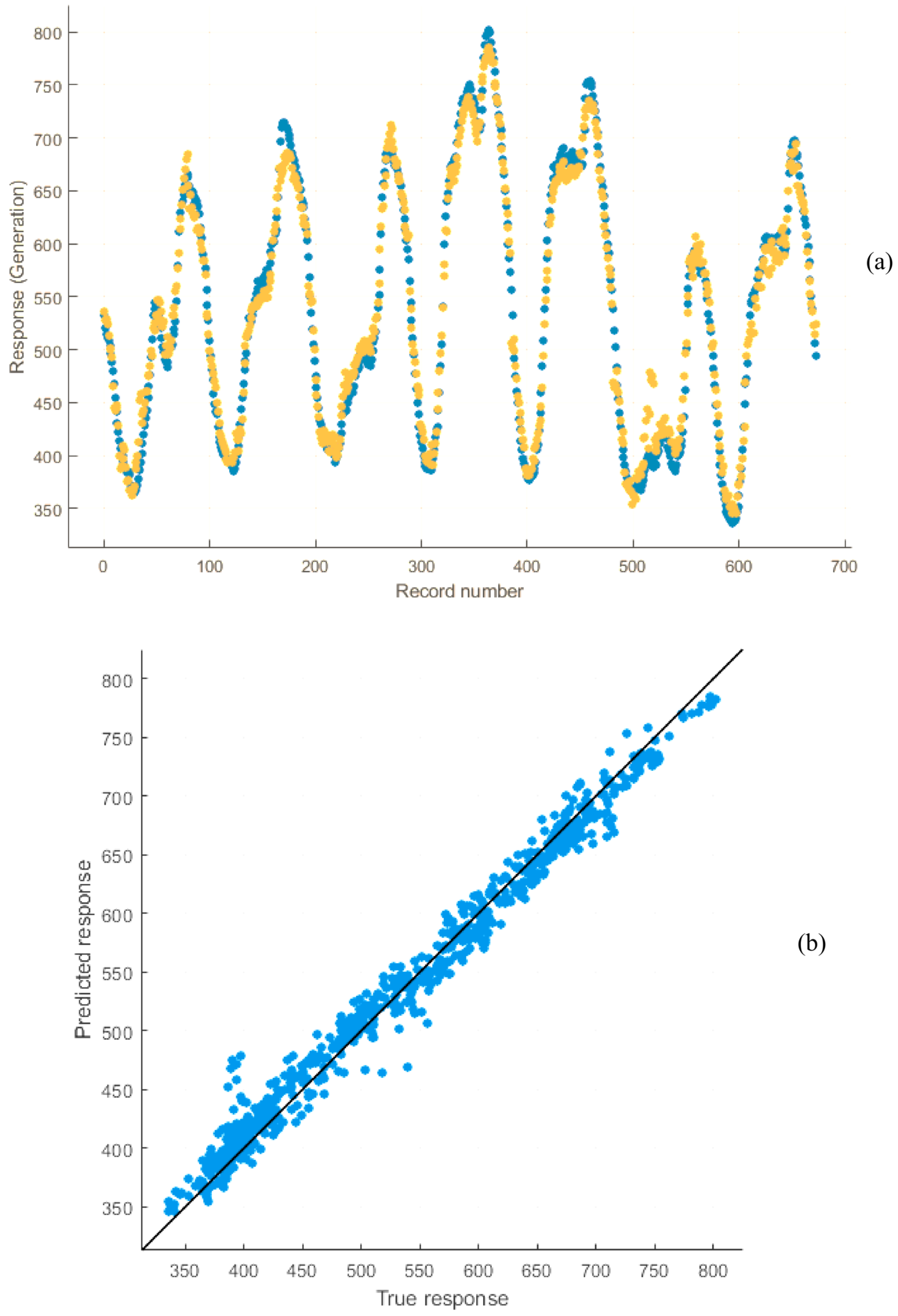
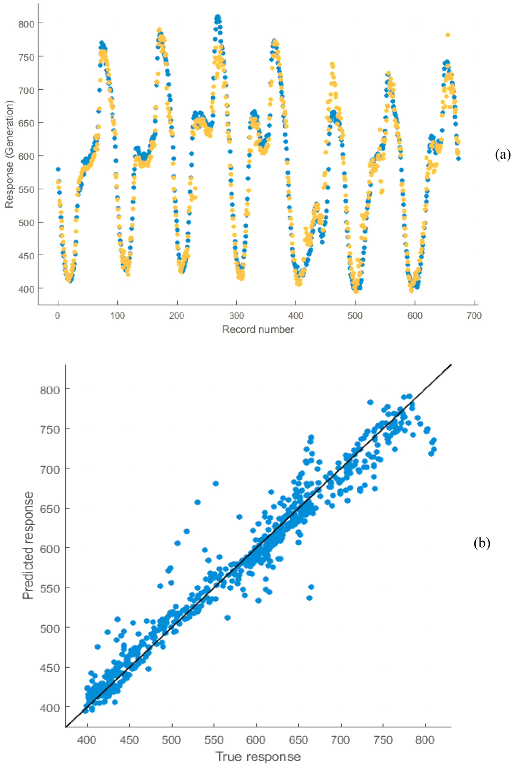
Figure 22 show the output generated via regression investigation for the training and testing datasets for long-term study. Figure 23 and Figure 24 show the output created by regression analysis for training and testing datasets for short-term training. The model responses (estimated) are designed against the targets (actual response). The greatest linear fitting is designated by the diagonal line. The results of the graphs show that predicted responses are not in good agreement with actual responses. It is concluded that the SVM method is not acceptable for this training. The average prediction errors of the SVM long-term model for 2016 and 2017 are 4.34% and 4.49%, and for the short-term model are 2.24% and 2.12%, respectively.

4. Methodology

The proposed forecasting procedure has three main phases: (a) determine the most suitable technique for estimating the electricity demand in Cyprus; (b) choose the best features that will provide the most information about the expected forecasting risk; and (c) offer recommendations for decision makers.
Step 1:
The inputs of the proposed forecasting model are electricity consumption of past months, temperature forecast, and various time features such as season and month of the year. This step includes data collection, its analysis, and extraction of its features.
Step 2:
The second step involves applying a simple seasonal exponential smoothing technique to forecast future temperature data that will be used as input in the regression model. Data are split into two sets: training and testing datasets. The training dataset is used to calculate the model parameters, while the testing dataset is utilized to measure the model’s performance.
Step 3:
In the third step, various machine learning techniques including SVR, ANN, ANFIS, and MLR are used to construct the forecasting models.
Step 4:
In the fourth step, the performance of the forecasting models is compared through the mean absolute percentage error, and the parameters are tuned to achieve the most accurate forecasting results.

5. Results and Discussion

In the current investigation, four models (artificial neural network (ANN), adaptive neuro-fuzzy inference system (ANFIS), support vector machine (SVM), and multiple linear regression (MLR)) are used to estimate electricity generation in Cyprus for the planning of power generation systems and the efficient operation and sustainable growth of modern electricity networks as long-term and short-term analysis. An ANN model for seven inputs and one output with a hidden layer including 80 nodes beginning from one node was fabricated and evaluated by utilizing the LM procedure. The model parameters were used for long-term and short-term analysis. For the 7-80-1 network with 1000 epochs, the model presented an optimal outcome. With additional nodes in the hidden layer and epochs, the result remained the same or somewhat expanded. Data division was random and Levenberg–Marquardt used as a training function.
In the ANFIS model, the gradient descent and least-squares algorithms are utilized for an operational examination of the optimal factors to achieve good outcomes. With respect to this cross method, connections of training and testing are improved. The Sugeno fuzzy design was made consistent with two IF rules. The ANFIS utilized in this investigation was settled with MATLAB. The ANFIS model includes 2160 fuzzy rules for long-term and 243 rules for short-term study. Furthermore, three generalized Gauss membership algorithms are utilized that diminish the handling time and provide improved outcomes for the estimation of electricity generation.
The SVM model is trained by utilizing the sequential optimization algorithm function and the kernel function utilized is the radial basis function. The MLR model was achieved from the repeated random subsampling procedure with 20 runs. Then, the MLR model with many iterations (1000) reached the ultimate forecast outcomes, and was used for the persistence of outcome assessment.
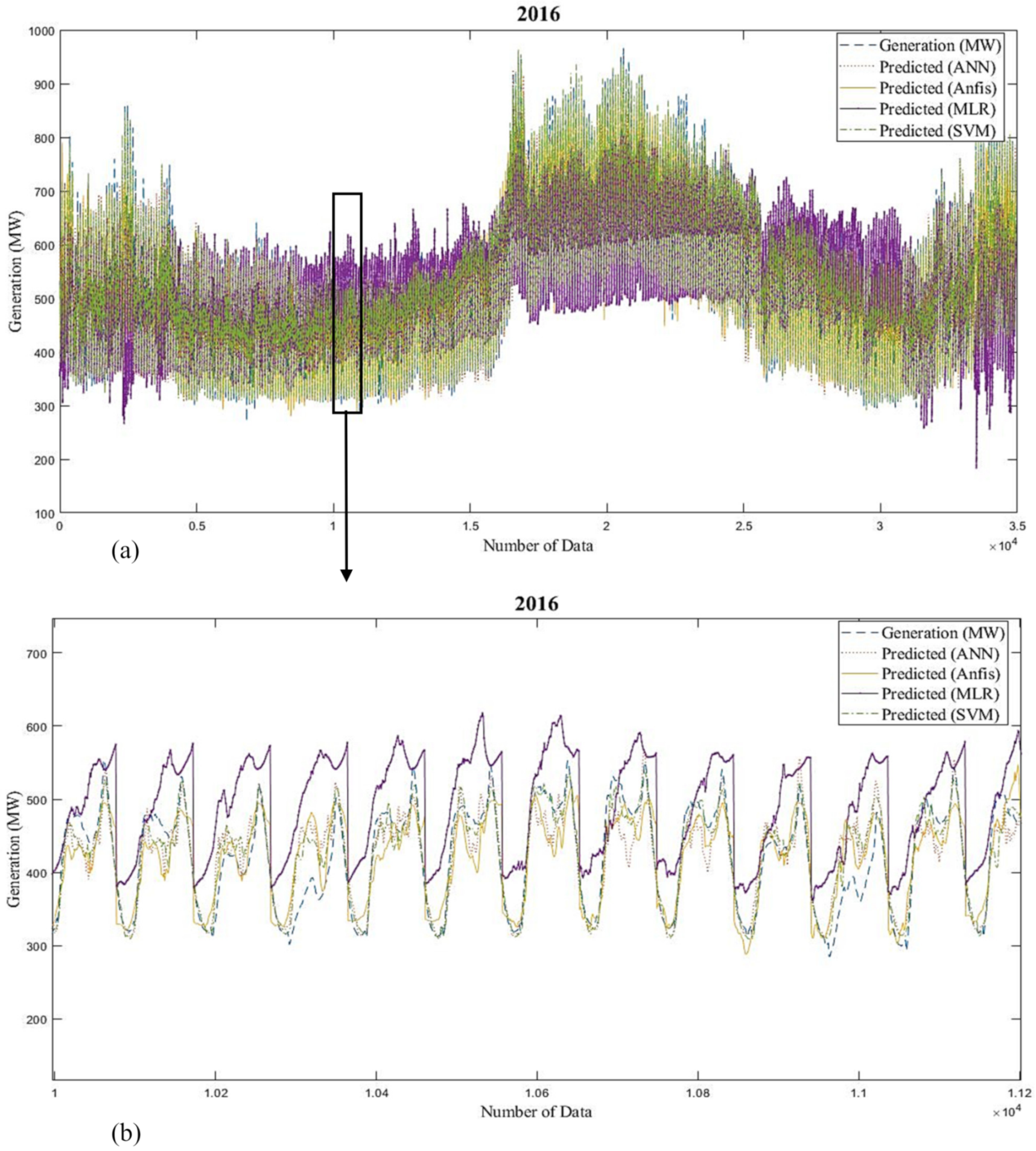
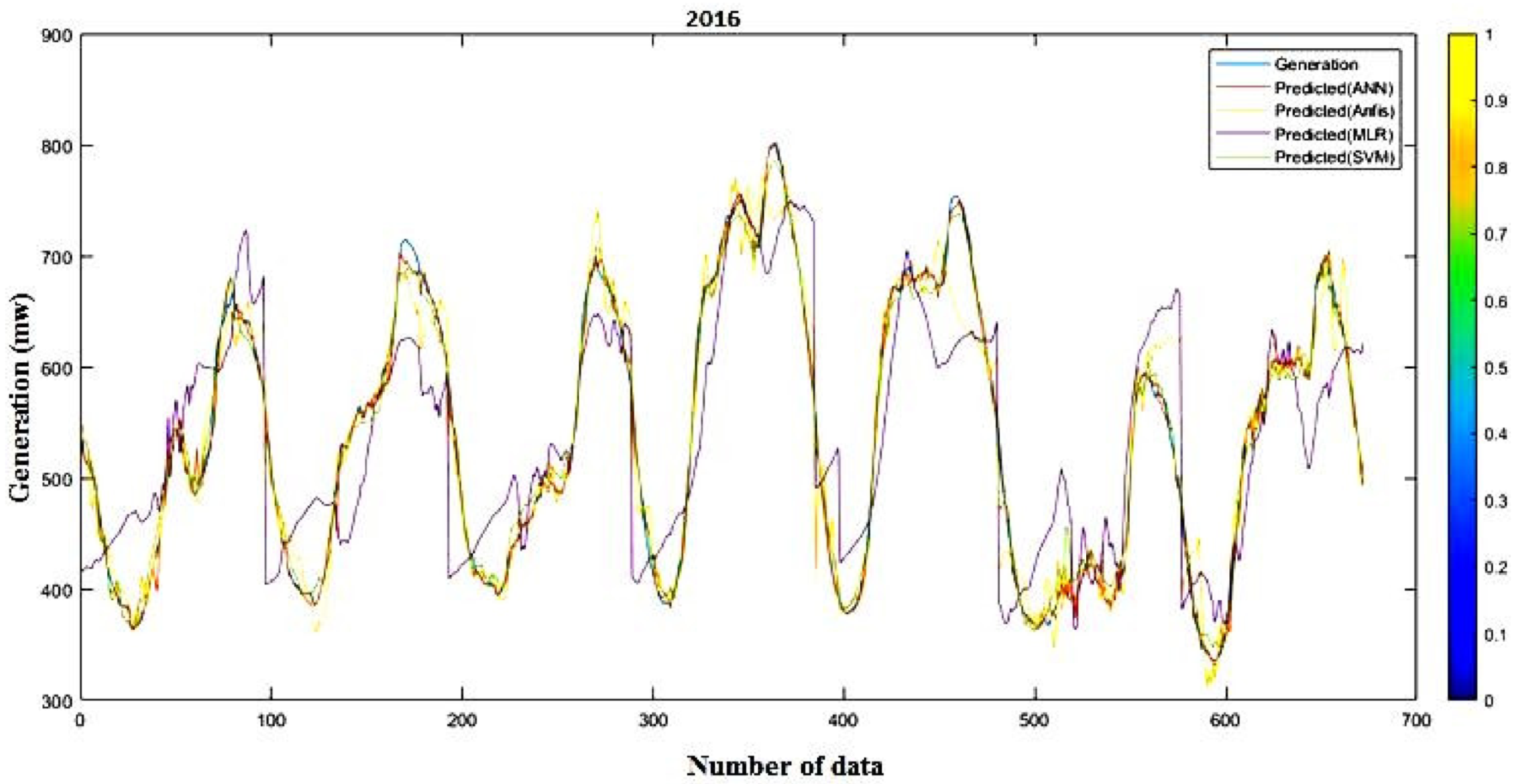
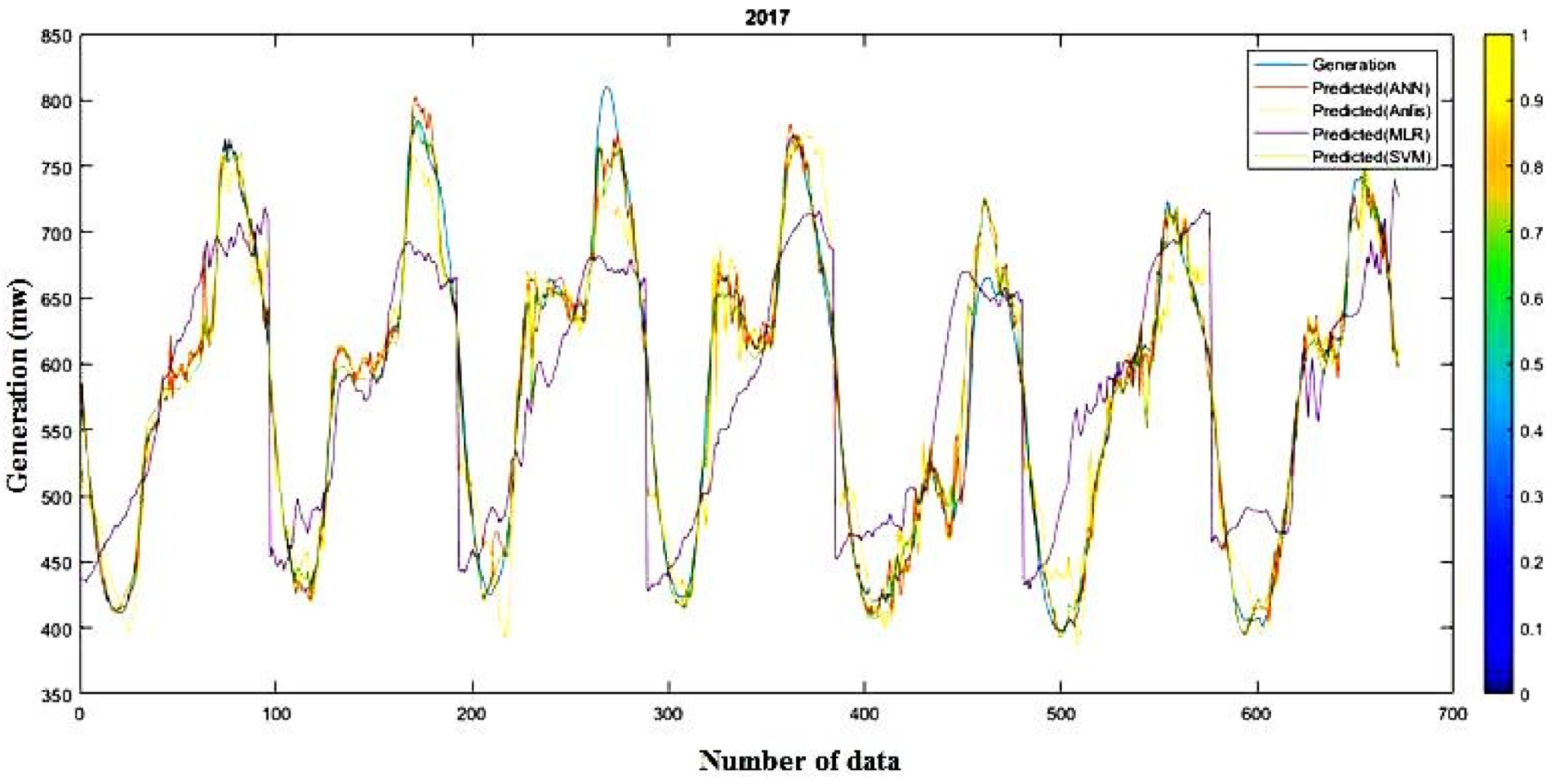
 Figure 25 and Figure 26 and Table 3; Table 4 show the predicted generation responses from ANN, ANFIS, MLR, and SVM models and the real responses in variable investigational situations for 2016 and 2017 (long-term).
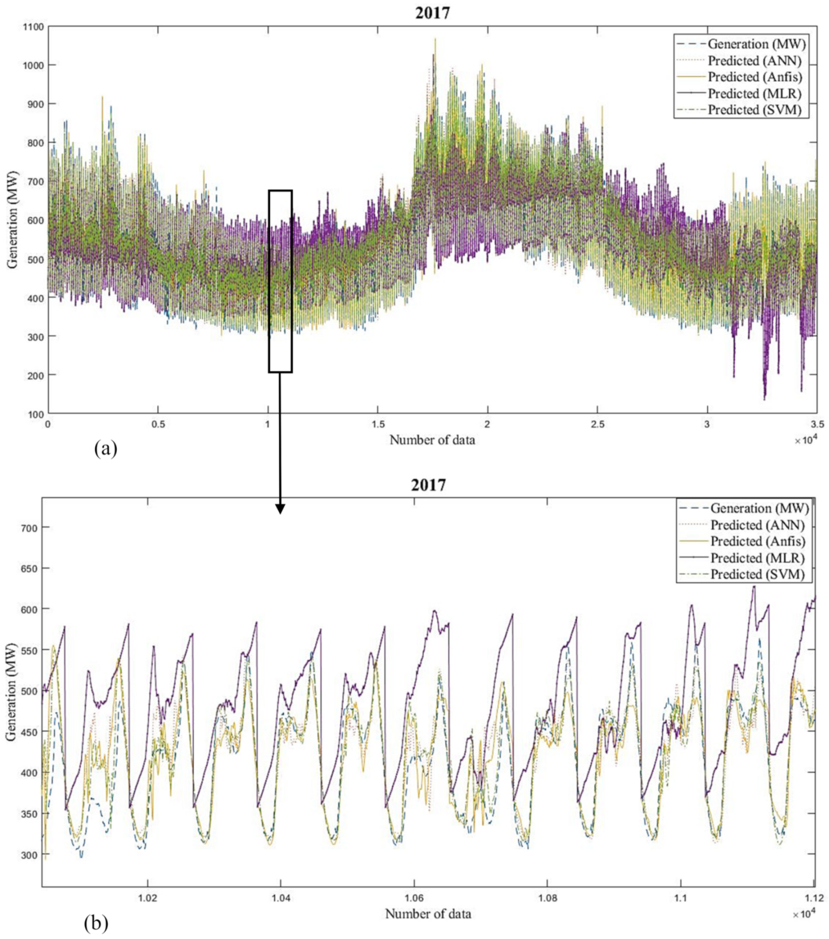
 Figure 27 and Figure 28 and Table 5 and Table 6 show the forecast generation results from the mentioned models and the actual outcomes in adaptable investigational conditions for 2016 and 2017 (short-term). Outcomes show that the actual responses are in near agreement with the predicted responses. The average prediction errors of ANN, ANFIS, MLR, and SVM models for long-term analysis are 5.57%, 7.69%, 15.18%, and 4.34% for 2016 and 5.28%, 6.11%, 13.4%, and 4.49% for 2017, which proves that the SVM and ANN models are relatively superior to other ML techniques. Additionally, Root Mean Square Error of the models proves the same result. Likewise, the defined errors of ANN, ANFIS, MLR, and SVM models for short-term study are 0.97%, 3.75%, 10.44%, and 2.24% for 2016 and 1.67%, 3.89%, 9.08%, and 2.12% for 2017, which shows that the ANN and SVM models are preferable over the other methods. Correspondingly, RMSE of the models proves that ANN is more superior to the other methods. The summery performance of all models are presented in Table 7.

6. Conclusions and Future Work

Load prediction has become increasingly important with the growth of the smart grid. It is a difficult task to predict the electricity load with high precision. The nonlinearity and volatility of real-time energy usage create difficulties in predicting energy demand and consumption. Precise load forecasting is crucial for the planning of power systems and operational decision making. In this study, machine learning approaches including artificial neural network (ANN), multiple linear regression (MLR), adaptive neuro-fuzzy inference system (ANFIS), and support vector machine (SVM) are applied to forecast the electricity load requirements in Cyprus.
It has been observed that electricity load is a function of temperature, humidity, solar irradiation, population, GNI per capita ($), and electricity price per kilowatt-hour; therefore, those were selected as the input parameters for the ML algorithms. The performance of the ML algorithms was comprehensively evaluated using electricity load data in Cyprus. A performance comparison among machine learning methods and identification of the importance of model input variables were carried out. Both the models’ accuracy of prediction and suitability for use were considered to support the forecast. The results indicate that SVM is relatively superior to other ML techniques, providing more reliable and accurate results in terms of lower prediction errors (4.34%, 4.49%) and Root Mean Square Error (25.43, 26.44) for long-term forecasting of energy generation requirements in Cyprus. The ANN model is better than other techniques for short-term analysis, providing lower prediction errors (0.97%, 1.67%) and RMSE (7.67, 14.91).
It is concluded that there is a strong link between energy demand, i.e., electricity load, economy, and environment, and predicting and forecasting electricity load is critical for planning future energy utilization in a sustainable manner.
It is anticipated that the results from this research can open roads toward future implementation of advanced calculation methods regarding energy demand and consumption. It is expected that such models will help energy planners to accurately plan for the future and utilize sustainable and renewable energy resources to a greater extent. The models will help policymakers and administrators to make decisions for a greener tomorrow. As for future work, LSTM and GRU methods can be applied to the time series existing in this research, meanwhile, this approach has achieved good outcomes in other time series forecasting problems.

Funding

This research received no external funding.

Conflicts of Interest

The author declares no conflicts of interest.

References

  1. Suganthi, L.; Samuel, A.A. Energy models for demand forecasting—A review. Renew. Sustain. Energy Rev. 2012, 16, 1223–1240. [Google Scholar] [CrossRef]
  2. Fan, C.; Wang, J.; Gang, W.; Li, S. Assessment of deep recurrent neural network-based strategies for short-term building energy predictions. Appl. Energy 2019, 236, 700–710. [Google Scholar] [CrossRef]
  3. Mashud, R.; Koprinska, I. Forecasting Electricity Load with Advanced Wavelet Neural Networks. Neurocomputing 2016, 182, 118–132. [Google Scholar]
  4. Friedrich, L.; Afshari, A. Short-term Forecasting of the Abu Dhabi electricity load using multiple weather variables. Energy Procedia 2015, 75, 3014–3026. [Google Scholar] [CrossRef] [Green Version]
  5. Zachariadis, T. Forecast of electricity consumption in Cyprus up to the year 2030: The potential impact of climate change. Energy Policy 2010, 38, 744–750. [Google Scholar] [CrossRef]
  6. Zachariadis, T. The Effect of Energy Efficiency Policies on the Medium-Term Energy Outlook of Cyprus. Cyprus Econ. Policy Rev. 2014, 8, 35–51. [Google Scholar]
  7. Amara, F.; Agbossou, K. Comparison and Simulation of Building Thermal Models for Effective Energy Management. Smart Grid Renew. Energy 2015, 6, 95–112. [Google Scholar] [CrossRef] [Green Version]
  8. Bourdeau, M.; Zhai, X.Q.; Nefzaoui, E.; Guo, X.; Chatellier, P. Modeling and Forecasting Building Energy Consumption: A Review of Data-Driven Techniques. Sustain. Cities Soc. 2019, 48, 101533. [Google Scholar] [CrossRef]
  9. Touretzky, C.R.; Patil, R. Building-level power demand forecasting framework using building specific inputs: Development and applications. Appl. Energy 2015, 147, 466–477. [Google Scholar] [CrossRef]
  10. Ferracuti, F.; Fonti, A.; Ciabattoni, L.; Pizzuti, S.; Comodi, G. Data-driven models for short-term thermal behaviour prediction in real buildings Research article. Appl. Energy 2017, 204, 1375–1387. [Google Scholar] [CrossRef]
  11. Ahmad, T.; Chen, H.; Guo, Y.; Wang, J. A comprehensive overview of the data-driven and large scale based approaches for forecasting of building energy demand: A review. Energy Build. 2018, 165, 301–320. [Google Scholar] [CrossRef]
  12. Ahmad, T.; Chen, H.; Shair, J. Water source heat pump energy demand prognosticate using disparate data-mining based approaches. Energy 2018, 152, 788–803. [Google Scholar] [CrossRef]
  13. Ahmad, T.; Chen, H.; Huang, R.; Guo, Y.; Wang, J.; Shair, J.; Akram, H.M.A.; Mohsan, S.A.H.; Kazim, M. Supervised based machine learning models for short, medium and long-term energy prediction in distinct building environment. Energy 2018, 158, 17–32. [Google Scholar] [CrossRef]
  14. He, W. Load forecasting via deep neural networks. Procedia Comput. Sci. 2017, 122, 308–314. [Google Scholar] [CrossRef]
  15. Hamlich, M.; eddine Belbounaguia, N. Short-Term Load Forecasting using Machine Learning and Periodicity Decomposition. AIMS Energy 2019, 7, 382–394. [Google Scholar]
  16. Shilpa, G.N.; Sheshadri, G.S. Short-term load forecasting using ARIMA model for Karnataka state electrical load. Int. J. Eng. Res. Dev. 2017, 13, 75–79. [Google Scholar]
  17. Dash, S.K.; Dash, P.K. Short-term mixed electricity demand and price forecasting using adaptive autoregressive moving average and functional link neural network. J. Mod. Power Syst. Clean Energy 2019, 7, 1241–1255. [Google Scholar] [CrossRef] [Green Version]
  18. Yu, X.; Bu, G.; Peng, B.; Zhang, C.; Yang, X.; Wu, J.; Zou, Z. Support Vector Machine Based on Clustering Algorithm for Interruptible Load Forecasting. IOP Conf. Series Mater. Sci. Eng. 2019, 533, 12018. [Google Scholar] [CrossRef]
  19. Lahouar, A.; Slama, J.B.H. Day-ahead load forecast using random forest and expert input selection. Energy Convers. Manag. 2015, 103, 1040–1051. [Google Scholar] [CrossRef]
  20. Bonanno, F.; Capizzi, G.; Sciuto, G.L.; Napoli, C.; Pappalardo, G.; Tramontana, E. A novel cloud-distributed toolbox for optimal energy dispatch management from renewables in igss by using wrnn predictors and gpu parallel solutions. In Proceedings of the 2014 International Symposium on Power Electronics, Electrical Drives, Automation and Motion, Ischia, Italy, 18–20 June 2014; pp. 1077–1084. [Google Scholar]
  21. Bonanno, F.; Capizzi, G.; Sciuto, G.L. A neuro wavelet-based approach for short-term load forecasting in integrated generation systems. In Proceedings of the 2013 International Conference on Clean Electrical Power (ICCEP), Alghero, Italy, 11–13 June 2013; pp. 772–776. [Google Scholar]
  22. Baz, W.E.; Tzscheutschler, P. Short-term smart learning electrical load prediction algorithm for home energy management systems. Appl. Energy 2015, 147, 10–19. [Google Scholar] [CrossRef]
  23. Zúñiga, K.; Castilla, I.; Aguilar, R. Using fuzzy logic to model the behavior of residential electrical utility customers. Appl. Energy 2014, 115, 384–393. [Google Scholar] [CrossRef]
  24. Gaur, M.; Majumdar, A. One-Day-Ahead Load Forecasting Using Nonlinear Kalman Filtering Algorithms, Special Section on: Current Research Topics in Power, Nuclear and Fuel Energy, SP-CRTPNFE 2016. In Proceedings of the International Conference on Recent Trends in Engineering, Science and Technology 2016, Hyderabad, India, 1 June 2016. [Google Scholar]
  25. Gheydi, M.; Nouri, A.; Ghadimi, N. Planning in microgrids with conservation of voltage reduction. IEEE Syst. J. 2016, 12, 2782–2790. [Google Scholar] [CrossRef]
  26. Ghadimi, N.; Akbarimajd, A.; Shayeghi, H.; Abedinia, O. Application of a New Hybrid Forecast Engine with Feature Selection Algorithm in a Power System. Int. J. Ambient Energy 2019, 40, 494–503. [Google Scholar] [CrossRef]
  27. Laouafi, A.; Mordjaoui, M.; Boukelia, T.E. An adaptive neuro-fuzzy inference system-based approach for daily load curve prediction. J. Energy Syst. 2018, 2, 115–126. [Google Scholar] [CrossRef]
  28. Sharifi, S.; Sedaghat, M.; Farhadi, P.; Ghadimi, N.; Taheri, B. Environmental Economic Dispatch using Improved Artificial Bee Colony Algorithm. Evolv. Syst. 2017, 8, 233–242. [Google Scholar] [CrossRef]
  29. Sakurai, D.; Fukuyama, Y.; Iizaka, T.; Matsui, T. Daily Peak Load Forecasting by Artificial Neural Network using Differential Evolutionary Particle Swarm Optimization Considering Outliers. IFAC-PapersOnLine 2019, 52, 389–394. [Google Scholar] [CrossRef]
  30. Gollou, A.R.; Ghadimi, N. A new feature selection and hybrid forecast engine for day-ahead price forecasting of electricity markets. J. Intell. Fuzzy Syst. Prepr. 2017, 32, 4031–4045. [Google Scholar] [CrossRef]
  31. Lu, H.; Azimi, M.; Iseley, T. Short-term load forecasting of urban gas using a hybrid model based on improved fruit fly optimization algorithm and support vector machine. Energy Rep. 2019, 5, 666–677. [Google Scholar] [CrossRef]
  32. Samuel, I.A.; Adetiba, E.; Odigwe, I.A.; Felly-Njoku, F.C. A comparative study of regression analysis and artificial neural network methods for medium-term load forecasting. Indian J. Sci. Tech. 2017, 10. [Google Scholar] [CrossRef]
  33. Cheepati, K.R.; Prasad, T.N. Performance comparison of short term load forecasting techniques. Int. J. Grid Distrib. Comput. 2016, 9, 287–302. [Google Scholar] [CrossRef]
  34. Tian, C.; Ma, J.; Zhang, C.; Zhan, P. A deep neural network model for short-term load forecast based on long short-term memory network and convolutional neural network. Energies 2018, 11, 3493. [Google Scholar] [CrossRef] [Green Version]
  35. Bozkurt, Ö.Ö.; Biricik, G.; Tayşi, Z.C. Artificial neural network and SARIMA based models for power load forecasting in Turkish electricity market. PLoS ONE 2017, 12, e0175915. [Google Scholar] [CrossRef] [Green Version]
  36. Zachariadis, T.; Pashourtidou, N. An empirical analysis of electricity consumption in Cyprus. Energy Econ. 2007, 29, 183–198. [Google Scholar] [CrossRef]
  37. Markou, M.; Kyriakides, E.; Polykarpou, M. 24-hour ahead short term load forecasting using multiple MLP. In Proceedings of the International Workshop on Deregulated Electricity Market Issues in South-Eastern Europe, Nicosia, Cyprus, 22–23 September 2008; pp. 1–6. [Google Scholar]
  38. Mirlatifi, A.M. Electricity Peak Demand Forecasting for Developing Countries. Ph.D. Thesis, Eastern Mediterranean University, Institute of Graduate Studies and Research, Dept. of Mechanical Engineering, Famagusta, North Cyprus, 2016. [Google Scholar]
  39. Kavaklioglu, K.; Ceylan, H.; Ozturk, H.K.; Canyurt, O.E. Modeling and prediction of Turkey’s electricity consumption using Artificial Neural Networks. Energy Convers. Manag. 2009, 50, 2719–2727. [Google Scholar] [CrossRef]
  40. Bouktif, S.; Fiaz, A.; Ouni, A.; Serhani, M.A. Optimal deep learning lstm model for electric load forecasting using feature selection and genetic algorithm: Comparison with machine learning approaches. Energies 2018, 11, 1636. [Google Scholar] [CrossRef] [Green Version]
  41. Faes, L.; Wagner, S.K.; Fu, D.J.; Liu, X.; Korot, E.; Ledsam, J.R.; Back, T.; Chopra, R.; Pontikos, N.; Kern, C.; et al. Automated deep learning design for medical image classification by health-care professionals with no coding experience: A feasibility study. Lancet Digit. Health 2019, 1, e232–e242. [Google Scholar] [CrossRef] [Green Version]
  42. Wuest, T.; Weimer, D.; Irgens, C.; Thoben, K.D. Machine learning in manufacturing: Advantages, challenges, and applications. Prod. Manuf. Res. 2016, 4, 23–45. [Google Scholar] [CrossRef] [Green Version]
  43. Kashyap, P. Industrial Applications of Machine Learning. In Machine Learning for Decision Makers; Apress: Berkeley, CA, USA, 2017. [Google Scholar] [CrossRef]
  44. Bâra, A.; Oprea, S.V. Electricity consumption and generation forecasting with artificial neural networks. In Advanced Applications for Artificial Neural Networks; El-Shahat, A., Ed.; IntechOpen: Rijeka, Croatia, 2017; pp. 119–141. [Google Scholar] [CrossRef] [Green Version]
  45. Li, K.; Hu, C.; Liu, G.; Xue, W. Building’s electricity consumption prediction using optimized artificial neural networks and principal component analysis. Energy Build. 2015, 108, 106–113. [Google Scholar] [CrossRef]
  46. Yuce, B.; Mourshed, M.; Rezgui, Y. A smart forecasting approach to district energy management. Energies 2017, 10, 1073. [Google Scholar] [CrossRef] [Green Version]
  47. Kumar, S.; Mishra, S.; Gupta, S. Short Term Load Forecasting using ANN and Multiple Linear Regression. In Proceedings of the Second International Conference on Computational Intelligence & Communication Technology (CICT), Ghaziabad, India, 12–13 February 2016; pp. 184–186. [Google Scholar]
  48. Raza, M.Q.; Khosravi, A. A review on artificial intelligence based load demand forecasting techniques for smart grid and buildings. Renew. Sustain. Energy Rev. 2015, 50, 1352–1372. [Google Scholar] [CrossRef]
  49. Ferrero Bermejo, J.; Gómez Fernández, J.F.; Olivencia Polo, F.; Crespo Márquez, A. A Review of the Use of Artificial Neural Network Models for Energy and Reliability Prediction. A Study of the Solar PV, Hydraulic and Wind Energy Sources. Appl. Sci. 2019, 9, 1844. [Google Scholar] [CrossRef] [Green Version]
  50. Staub, S.; Karaman, E.; Kaya, S.; Karapınar, H.; Güven, E. Artificial Neural Network and Agility. Proc. Soc. Behav. Sci. 2015, 195, 1477–1485. [Google Scholar] [CrossRef] [Green Version]
  51. Aydinalp, M.; Ismet Ugursal, V.; Fung, A.S. Modeling of the appliance, lighting, and space-cooling energy consumptions in the residential sector using neural networks. Appl. Energy 2002, 71, 87–110. [Google Scholar] [CrossRef]
  52. Jones, A.H.S.; Pranolo, A.; Dianto, A.; Winiarti, S. Prediction of Population Growth using Sugeno and Adaptive Neuro-Fuzzy Inference System (ANFIS). In IOP Conference Series: Materials Science and Engineering; IOP Publishing: Bristol, UK, 2018; Volume 403, p. 12073. [Google Scholar]
  53. Anderson, D.R.; Sweeney, D.J.; Williams, T.A. Modern Business Statistics with Microsoft Excel, 5th ed.; Protoview; Cengage Learning: Boston, MA, USA, 2014; Volume 1. [Google Scholar]
  54. Braun, M.R.; Altan, H.; Beck, S.B.M. Using regression analysis to predict the future energy consumption of a supermarket in the UK. Appl. Energy 2014, 130, 305–313. [Google Scholar] [CrossRef] [Green Version]
  55. Baltputnis, K.; Petrichenko, R.; Sobolevsky, D. Heating demand forecasting with multiple regression: Model setup and case study. In Proceedings of the 2018 IEEE 6th Workshop on Advances in Information, Electronic and Electrical Engineering (AIEEE), Vilnius, Lithuania, 8–10 November 2018; pp. 1–5. [Google Scholar]
  56. Aleksandar, P.; Silvana, P.; Valentina, Z.P. Multiple Linear Regression Model. for Predicting Bidding Price. Tech. Technol. Educ. Manag. 2015, 10, 143–151. [Google Scholar]
  57. Ma, Z.; Ye, C.; Li, H.; Ma, W. Applying support vector machines to predict building energy consumption in China. Energy Procedia 2018, 152, 780–786. [Google Scholar] [CrossRef]
  58. Gandhi, R. Retrieved 11 April 2019, from towards Data Science Website. Introduction to Machine Learning Algorithms: Linear Regression. Available online: https://towardsdatascience.com/ (accessed on 28 April 2020).
  59. Vinagre, E.; Pinto, T.; Ramos, S.; Vale, Z.; Corchado, J.M. Electrical energy consumption forecast using support vector machines. In Proceedings of the 2016 27th International Workshop on Database and Expert Systems Applications (DEXA), Porto, Portugal, 5–8 September 2016; pp. 171–175. [Google Scholar]
  60. Guo, L.; Chen, J.; Wu, F.; Wang, M. An electric power generation forecasting method using support vector machine. Syst. Sci. Control Eng. 2018, 6, 191–199. [Google Scholar] [CrossRef] [Green Version]
  61. Fu, Y.; Li, Z.; Zhang, H.; Xu, P. Using support vector machine to predict next day electricity load of public buildings with sub-metering devices. Procedia Eng. 2015, 121, 1016–1022. [Google Scholar] [CrossRef] [Green Version]
Figure 1. Classification of machine learning algorithms: Generalized linear model (GLM); Support Vector Regression (SVR), Gaussian Process Regression (GPR).
Sustainability 12 03612 g001
Figure 2. (a) The ANN model. (b) The Neural Network Architecture. (c) The percentage of the divided dataset.
Sustainability 12 03612 g002
Figure 3. Plots of data regression for 2016 datasets (long-term). (a) Plot of data regressions (training set). (b) Plot of data regressions (validating set). (c) Plot of data regressions (testing set). (d) Plot of data regressions (all).
Sustainability 12 03612 g003
Figure 4. Plots of data regression for 2017 datasets (long-term). (a) Plot of data regressions (training set). (b) Plot of data regressions (validating set). (c) Plot of data regressions (testing set). (d) Plot of data regressions (all).
Sustainability 12 03612 g004
Figure 5. Plots of data regression for 2016 datasets (short-term). (a) Plot of data regressions (training set). (b) Plot of data regressions (validating set). (c) Plot of data regressions (testing set). (d) Plot of data regressions (all).
Sustainability 12 03612 g005
Figure 6. Plots of data regression for 2017 datasets (short-term). (a) Plot of data regressions (training set). (b) Plot of data regressions (validating set). (c) Plot of data regressions (testing set). (d) Plot of data regressions (all).
Sustainability 12 03612 g006
Figure 7. Established fuzzy model.
Sustainability 12 03612 g007
Figure 8. Design of an adaptive neuro-fuzzy inference system (ANFIS) model for generation.
Sustainability 12 03612 g008
Figure 9. Three-dimensional graphs of generation values (2016, long-term). (a) Solar vs. temperature. (b) Population vs. solar. (c) Population vs. humid. (d) Humid vs. temperature. (e) Population vs. temperature. (f) Solar vs. Humid.
Sustainability 12 03612 g009
Figure 10. Three-dimensional graphs of generation values (2017, long-term). (a) Solar vs. temperature. (b) Population vs. solar. (c) Population vs. humid. (d) Humid vs. temperature. (e) Population vs. temperature. (f) Humid vs. Solar.
Sustainability 12 03612 g010
Figure 11. Three-dimensional graphs of generation values (2016, short-term). (a) Solar vs. temperature. (b) Population vs. solar. (c) Population vs. humid. (d) Humid vs. temperature. (e) Population vs. temperature. (f) Solar vs. Humid.
Sustainability 12 03612 g011
Figure 12. Three-dimensional graphs of generation values (2017, short-term). (a) Solar vs. temperature. (b) Population vs. solar. (c) Population vs. humid. (d) Humid vs. temperature. (e) Population vs. temperature. (f) Solar vs. Humid.
Sustainability 12 03612 g012
Figure 13. (a) Estimated vs. actual values for generation (2016, long-term). (b) The zoomed part of the graph.
Sustainability 12 03612 g013
Figure 14. (a) Estimated vs. actual values for generation (2017, long-term). (b) The zoomed part of the graph.
Sustainability 12 03612 g014
Figure 15. Estimated vs. actual values for generation (2016, short-term).
Sustainability 12 03612 g015
Figure 16. Estimated vs. actual values for generation (2017, short-term).
Sustainability 12 03612 g016
Figure 17. (a) Linear multiple linear regression (MLR) results for predicted values versus true responses (2016, long-term). (b) The zoomed part of the graph. (c) Plotting Cross-Validated Predictions.
Sustainability 12 03612 g017aSustainability 12 03612 g017b
Figure 18. (a) Linear MLR results for predicted values versus true responses (2017, long-term). (b) The zoomed part of the graph. (c) Plotting Cross-Validated Predictions.
Sustainability 12 03612 g018aSustainability 12 03612 g018b
Figure 19. (a) Linear MLR results for predicted values versus true responses (2016, short-term). (b) Plotting Cross-Validated Predictions.
Sustainability 12 03612 g019
Figure 20. (a) Linear MLR results for predicted values versus true responses (2017, short-term). (b) Plotting Cross-Validated Predictions.
Sustainability 12 03612 g020
Figure 21. (a) Linear support vector machine (SVM) results for predicted values versus true responses (2016). (b) The zoomed part of the graph. (c) Plotting Cross-Validated Predictions.
Sustainability 12 03612 g021aSustainability 12 03612 g021b
Figure 22. (a) Linear SVM results for predicted values versus true responses (2017). (b) The zoomed part of the graph. (c) Plotting Cross-Validated Predictions.
Sustainability 12 03612 g022
Figure 23. (a) Linear SVM results for predicted values versus true responses (2016, short-term). (b) Plotting Cross-Validated Predictions.
Sustainability 12 03612 g023
Figure 24. (a) Linear SVM results for predicted values versus true responses (2017, short term). (b) Plotting Cross-Validated Predictions.
Sustainability 12 03612 g024
Figure 25. (a) Variation of generation values with amount of data (2016, long-term). (b) The zoomed part of the graph.
Sustainability 12 03612 g025
Figure 26. (a) Variation of generation values with amount of data (2017, long-term). (b) The zoomed part of the graph.
Sustainability 12 03612 g026
Figure 27. Variation of generation values with amount of data (2016, short-term).
Sustainability 12 03612 g027
Figure 28. Variation of generation values with amount of data (2017, short-term).
Sustainability 12 03612 g028
Table 1. Summary of models used in the literature for energy and electricity peak demand forecasting in Cyprus.
Zachariadis [36]Forecast of electricity consumptionSingle-equation auto-regressive distributed lag (ARDL) modelsCyprusBased on econometric analysis of energy use as a function of macroeconomic variables, prices, and weather conditions
Markou et al. [37]Electricity demand forecastArtificial neural network (ANN)CyprusSignificant factors: quarter-hour load generation, temperature, and humidity values
Mirlatifi [38]Electricity peak demand forecastFuzzy peak demand forecastingCyprusMany parameters, such as economic, environmental, or political situations, can affect demand
Table 2. Data Feature.
Long TermShort Term
2016201720162017
One yearOne yearOne week (Jan)One week (Jan)
34,944 (data set)34,944 (data set)673 (data set)673 (data set)
Table 3. Predicted ANN, ANFIS, MLR, and SVM for generation (2016, long-term). GNI, gross national income.
Predict
NumberHourTemp. (°C)Humid. (%)Solar (W/m2)GNI per Capita ($)Population (k)Electricity Price (kWh)Generation (MW)ANNANFISMLRSVM
100:00386.7021,274851.611.96533606.48424.90356.43517.82
200:152.987021,274851.611.96520587.45425.08360.31501.46
300:303.285.4021,274851.611.96514557.87425.51360.01487.97
400:453.383.1021,274851.611.96511530.22428.05358.57482.89
501:003.480021,274851.611.96509502.74432.14355.62480.54
601:153.578.2021,274851.611.96504502.67434.48355.27470.74
701:303.480.7021,274851.611.96497483.05431.24363.26450.96
801:453.281.4021,274851.611.96488470.20431.41367.87438.78
902:003.477.3021,274851.611.96480470.08436.89362.88442.85
1002:153.474.9021,274851.611.96468454.29440.93361.32438.25
1102:303.375.4021,274851.611.96455451.09440.97365.40431.95
1202:452.877.8021,274851.611.96442446.79440.12373.41426.64
1303:002.679.1021,274851.611.96431437.86439.72379.40416.30
1403:152.577.1021,274851.611.96422433.47444.01378.43420.23
1503:302.773.7021,274851.611.96414421.79449.12374.46416.74
1603:45372.1021,274851.611.96407418.02450.53374.41407.90
1704:003.173.7021,274851.611.96402416.28448.44380.82404.70
1804:152.976.2021,274851.611.96399412.89446.67389.13399.86
1904:302.678021,274851.611.96395424.90446.45396.28394.19
2004:452.477.7021,274851.611.96390424.72449.16399.03396.25
2105:002.375.9021,274851.611.96387410.48454.01398.45400.79
34,94423:45:006.693.6021,274866.511.96521623.02707.30635.59603.31
Prediction error %5.577.6915.184.34
Root Mean Square Error (RMSE)29.9541.4767.5425.43
Table 4. Predicted ANN, ANFIS, MLR, and SVM for generation (2017, long-term).
Predict
NumberHourTemp. (°C)Humid. (%)Solar (W/m2)GNI per Capita ($)Population (k)Electricity Price (kWh)Generation (MW)ANNANFISMLRSVM
100:003.892.4022,239859.513.72579588.64517.34422.41586.76
200:153.792.5022,239859.513.72561563.86514.85426.86570.06
300:303.592.9022,239859.513.72544541.71512.35432.27553.02
400:453.693.1022,239859.513.72525520.27508.57434.40536.50
501:003.593.2022,239859.513.72507503.55505.56438.91521.48
601:153.593.5022,239859.513.72492487.36501.81442.13506.65
701:303.593.7022,239859.513.72479473.31497.99445.41493.10
801:453.693.7022,239859.513.72466461.27493.74447.63480.50
902:003.693.9022,239859.513.72454450.14489.69450.90469.18
1002:153.793.9022,239859.513.72448440.99485.23453.09458.70
1102:303.793.9022,239859.513.72437433.50481.15456.49449.76
1202:453.793.6022,239859.513.72432428.42477.22460.10441.88
1303:003.793.4022,239859.513.72427420.15469.33463.64435.02
1403:153.793.1022,239859.513.72422417.91465.67467.25429.16
1503:303.692.7022,239859.513.72419417.32462.80472.17424.97
1603:453.692.8022,239859.513.72414416.20459.51475.51421.42
1704:003.792.8022,239859.513.72413414.92456.07477.65418.14
1804:153.792.4022,239859.513.72412415.63453.72481.33416.42
1904:303.592.4022,239859.513.72412418.91452.91487.28417.79
2004:453.592.4022,239859.513.72412420.44451.51490.70418.61
2105:003.592.4022,239859.513.72411422.39450.70494.12420.62
34,94423:45:006.693.6022,239866.513.72521514.95499.72521.11506.46
Prediction error %5.286.1113.44.49
Root Mean Square Error (RMSE)28.2733.3157.4526.44
Table 5. Predicted ANN, ANFIS, MLR, and SVM for generation (2016, short-term).
Predict
NumberHourTemp. (°C)Humid. (%)Solar (W/m2)GNI per Capita ($)Population (k)Electricity Price (kWh)Generation (MW)ANNANFISMLRSVM
100:00386.7021,274851.611.96533527.71547.51416.29536.33
200:152.987021,274851.611.96520518.08537.95417.73533.64
300:303.285.4021,274851.611.96514512.61535.15420.04530.71
400:453.383.1021,274851.611.96511512.84515.49419.83525.42
501:003.480021,274851.611.96509515.98487.1418.43513.74
601:153.578.2021,274851.611.96504509.69468.71418.58500.85
701:303.480.7021,274851.611.96497497.33484.1424.01502.47
801:453.281.4021,274851.611.96488487.32482.35426.37498.05
902:003.477.3021,274851.611.96480479.98455.07425.01471.28
1002:153.474.9021,274851.611.96468460.87441.86425.07451.21
1102:303.375.4021,274851.611.96455453.04442.86428.33443.09
1202:452.877.8021,274851.611.96442448.57451.13432.19445.25
1303:002.679.1021,274851.611.96431433.35438.42434.31447.44
1403:152.577.1021,274851.611.96422418.65436.83436.36425.22
1503:302.773.7021,274851.611.96414402.74433.72438.75399.12
1603:45372.1021,274851.611.96407396.15422.53440.35390.24
1704:003.173.7021,274851.611.96402398.25417.23443.32388.68
1804:152.976.2021,274851.611.96399400.23414.56446.41396.29
1904:302.678021,274851.611.96395393.55403.38447.91407.71
2004:452.477.7021,274851.611.96390386.34396.08449.62403.72
2105:002.375.9021,274851.611.96387384.67398.35452.7388.32
67323:457.487.7021,274851.711.96494499.03512.85621.6510.7
Prediction error %0.973.7510.442.24
Root Mean Square Error (RMSE)7.6728.8744.7113.4
Table 6. Predicted ANN, ANFIS, MLR, and SVM for generation (2017, short-term).
Predict
NumberHourTemp. (°C)Humid. (%)Solar (W/m2)GNI per Capita ($)Population (k)Electricity Price (kWh)Generation (MW)ANNANFISMLRSVM
100:003.892.4022,239859.513.72579585.14519.02436.39565.29
200:153.792.5022,239859.513.72561565.18510.06436.75552.26
300:303.592.9022,239859.513.72544542.67497.25434.53537.11
400:453.693.1022,239859.513.72525526.49501.03438.95526.24
501:003.593.2022,239859.513.72507510.58492.2439.23513.45
601:153.593.5022,239859.513.72492494.76489.49441.41501.61
701:303.593.7022,239859.513.72479480.71485.9443.74490.32
801:453.693.7022,239859.513.72466469.76486.15448.58479.6
902:003.693.9022,239859.513.72454457.25481.33450.96469.32
1002:153.793.9022,239859.513.72448447.49479.89455.88459.52
1102:303.793.9022,239859.513.72437438.79473.55458.51450.19
1202:453.793.6022,239859.513.72432434.15466.92461.44440.78
1303:003.793.4022,239859.513.72427422.91453.96464.24432.68
1403:153.793.1022,239859.513.72422420.44448.03467.12425.57
1503:303.692.7022,239859.513.72419418.97442.82467.74420.98
1603:453.692.8022,239859.513.72414415.03436.78470.22416.91
1704:003.792.8022,239859.513.72413413.38430.21475.14412.85
1804:153.792.4022,239859.513.72412415.74426.73477.9411.5
1904:303.592.4022,239859.513.72412413.72425.39475.87414.55
2004:453.592.4022,239859.513.72412414.29420.87478.41415.45
2105:003.592.4022,239859.513.72411415.62416.48480.94417.44
67323:456.877.4022,239859.713.72596598.7613.17726.51609.56
Prediction error %1.673.899.082.12
Root Mean Square Error (RMSE)14.9131.0142.6717.47
Table 7. Root Mean Square Error (RMSE).
ANNANFISMLRSVM
Long term201629.9541.4767.5425.43
201728.2733.3157.4526.44
Short term20167.6728.8744.7113.4
201714.9131.0142.6717.47

