Energy-Efficient and Integrated Allocation of Berths, Quay Cranes, and Internal Trucks in Container Terminals

Abstract

Despite a significant number of studies that have focused on the operational efficiency of container terminals, existing literature has paid little attention to improving energy efficiency, e.g., energy consumption and negative externalities in container terminals. Most researchers consider energy-saving goals when allocating berths and quay cranes to vessels, assuming that internal trucks are in sufficient supply. Furthermore, recent studies have revealed that shortage of internal trucks has become an issue that greatly affects the operational and energy efficiencies of container terminals. This work presents a planning model that integrates berth allocation, quay crane assignment, and internal truck assignment problems. The developed model contributes to existing literature by including energy-saving goals in the integrated planning of these problems, as well as including important realistic factors such as shortages of internal trucks and handling time estimations, thus producing a reliable handling plan that achieves energy and cost savings without additional truck investment. To solve realistic problems, a Lagrangian relaxation-based method is developed. Furthermore, the benefits of the developed approach are demonstrated by comparing it to an existing approach. On average, our approach could improve the solutions of the integrated problem with different numbers of internal trucks by 6% compared to the solutions obtained using the existing approach.

1. Introduction

Today, maritime transport has become an essential element of supply chains of services and products: more than 80% of global freight transport is by sea. It is expected that global maritime trade will increase, with an average annual growth rate of 3.5%, within the 2019–2024 period due to the increase in containerized, dry bulk, and gas cargos [1]. This in turn will lead to more pressure on seaports to accommodate the growing demand and provide adequate services with limited resource capacities. At a container terminal, once the vessel is settled at the quay, quay cranes (QCs) and internal trucks (ITs) are used to handle the containers on the vessel. The QC loads or unloads the containers to or from the IT, which transports the container from or to the storage area, where the IT is loaded or unloaded by the yard crane. The IT will repeatedly make this round trip until all containers on the vessels are handled. Accordingly, the handling time of the vessel is greatly affected by its assigned numbers of QCs and ITs. Existing studies have used two different names for the manned trucks that move containers between the quay side and yard side: yard trucks [2] and internal trucks [3]. In this paper, we use “internal trucks” to describe manned container trucks. Berths, QCs, and ITs are expensive resources at container terminals [4]. Therefore, there are considerable studies that have focused on the planning decisions related to these resources [5,6]. The berth allocation problem (BAP) determines the berthing schedule for each vessel. Typically, the berthing schedule is developed based on the estimated values of vessels’ handling times. The berthing schedule of a vessel describes its berthing position, berthing time, and completion time. The quay crane assignment problem (QCAP) calculates how many QCs are assigned to each vessel, while the internal truck assignment problem (ITAP) calculates how many ITs are assigned to the QCs that handle the containers on the vessel. The QCAP and ITAP together determine the handling times of the vessels, so that a specific objective is achieved.

With increasing numbers of containers, more resources are needed for container handling operations. However, purchasing additional resources is not an easy decision due to the high investment costs of these resources. Therefore, optimizing terminal operations has become necessary for container terminals to improve vessel service time, which is as an important measure of service quality [7]. The increasing demand for maritime transport has also led to more energy consumption and its related environmental impacts, such as greenhouse gas (GHG) emissions. For seaports, significant overhead costs are caused by energy consumption, and therefore, it is essential to reduce energy consumption to achieve more cost reduction and profits. At the same time, reducing energy consumption can support the transition toward greener and more sustainable container terminals, which has been of global concern [8,9]. Handling equipment and container vessels are often operated by diesel engines, which are significant sources of emissions and energy consumption in the port environment. The operational efficiency of container terminals (e.g., short service times) is highly dependent on effective planning of the handling operations of vessels using the available berths, QCs, and ITs [10]. Some studies have shown that improving the operational efficiency (minimizing vessel service time) might lead to energy savings. This is possible if there is a positive correlation between the two objectives, for example, vessels usually consume fuel while in idle mode for lighting purposes, refrigerating goods, and other onboard service purposes. A vessel is in idle mode when it is at port waiting for its service to start. Therefore, reducing the time that a vessel waits until its service starts can directly reduce the energy consumed during idle mode [11]. However, a negative correlation may exist between the two objectives. For example, vessels may arrive at a terminal late, and to reduce their waiting times, vessels may be allocated to available berths on a first-come, first-serve basis. Although this can reduce idle-mode energy consumption, this can cause more energy consumption on the part of ITs if the assigned berths are far from the dedicated yard areas for containers from vessels [12]. Therefore, recent literature has considered the tradeoff between energy-saving objectives and time-saving objectives when making plans for vessel handling operations [13].

There is a tight interrelation between the BAP, the QCAP, and the ITAP [14]. Existing studies have mostly focused on combining the BAP and the QCAP into a unified model called the integrated berth allocation and crane assignment problem (BACAP) [12,15,16,17]. For a detailed review on BACAP studies, we refer the readers to the recent survey in Reference [5]. Energy-saving objectives are often implemented by adapting green practices and policies to reduce carbon dioxide emissions [3]. Few studies have addressed the BACAP while considering energy savings to be a part of objective functioning [11,13,18,19]. These studies have aimed to create effective handling plans that achieve a good service level (minimization of the total delay in departure for vessels) as well as energy savings (minimization of energy consumption) in the operations of vessels and QCs. Reducing the amount of energy consumed by activated QCs can be achieved by reducing the total departure delays of all vessels [16]. This is because minimizing the total departure delays of all vessels can lead to minimizing the unproductive times of QCs, resulting in improving QCs’ energy consumption. Other studies have considered the energy consumption of QCs through the minimization of the number of QCs assigned to the vessels [13,19]. In order to minimize vessel fuel consumption while at port, relevant studies on BACAP have followed an emissions mitigation strategy that requires minimizing vessel waiting times [11].

In the majority of the works mentioned above, estimations of vessel handling times were made based on the number of containers to be handled, the assigned number of QCs, and the QCs’ average handling rates (container moves/hour). It is worth noting that QCs’ handling rates are highly dependent on the assigned number of ITs [20]. However, most studies have assumed that ITs are enough to supply the activated QCs with their truck needs [19,21]. Thus, the ITAP is ignored by this assumption.

Taking IT capacity constraints into account when planning handling operations has become crucial in adapting to recent changes in maritime logistics [22]. In the following section, we illustrate some examples of these recent changes. Many countries have recently witnessed a significant shortage in available truck drivers [23], which in turn constrains the capacity of ITs. As another example, recently it was noted that the port of Hong Kong is in serious need of more truck drivers because 59% of employed drivers have approached their retirement age and replacements are lacking [24]. Additional examples include deactivating some ITs due to maintenance activities [25]. On the other hand, labor costs are often in the range from 50% to 75% of total operation expenses in seaports [26]. Thus, it is not a cost-effective investment to maintain a complete set of drivers and/or ITs, especially when vessels’ calling frequency fluctuate greatly [27].

In the literature, the shortage of ITs is rarely considered. In general, outsourcing and sharing IT strategies have been most frequently proposed as solutions for truck shortages. Wang et al. [25] have developed a mathematical formulation for truck scheduling and storage space allocation problems with consideration of outsourcing ITs to external companies. Their proposed model seeks to find the daily number of outsourced trucks to minimize the shift between the planned and actual completion times of vessels. Sharing ITs suits ports with multiple container terminals whose locations must be adjacent to each other, making it possible to move ITs between terminals in little time. He et al. [4] created a mathematical formulation to make decisions on IT sharing between multiple container terminals in a large port. Their formulation can be used to find the number of ITs that can be shared between terminals in a given time period. More recently, Karam and Attia [28] presented a mathematical model for truck scheduling, taking into account IT sharing and outsourcing strategies to solve the issue of a lack of ITs in adjacent container terminals. However, if the operation planner cannot solve the issue of a lack of ITs using sharing and outsourcing strategies, planning handling operations has to be done taking into account the shortage of ITs. In this case, because the traditional method of estimating the vessels’ handling times ignores truck capacity constraints, the estimated handling times will be unreliable and often are lower than the true values. This in turn will delay the handling operations of successive vessels and may also delay the departure dates of the vessels. Therefore, the operation costs may increase due to delay penalties and higher energy consumption.

Very few studies have considered the shortage of ITs when making plans for berth allocation and quay crane assignments in container terminals. Karam et al. [29] developed a mathematical model for integrating the QCAP as well as the ITAP simultaneously. They showed the benefits of their proposed model compared to the traditional planning method. In an extended version of the model, they considered how to determine the specific QCs assigned to each vessel and proposed a heuristic-based solution to solve real problems [30]. More recently, Vahdani et al. [22] presented a two-objective optimization approach for simultaneous integration of the QCAP as well as the ITAP that considered the sharing of ITs between adjacent container terminals. Their model aimed to overcome the limited availability of ITs by sharing them among different terminals. None of these previous studies considered the BAP when integrating the QCAP and the ITAP. To date, integrating the BAP, the QCAP, and the ITAP has only been studied by Karam and Eltawil [31]. They developed a mathematical model for an integrated solution of BAP, QCAP, and ITAP. Their model aims to minimize the average service time of arriving vessels. In addition, they validated their model by comparing it to the BACAP model proposed by Meisel and Bierwith [12], assuming that ITs are available. In addition, their model was validated through a comparison to a queuing model proposed by Kang et al. [32] under limited availability of ITs. Based on the current state of the literature, it is obvious that the lack of integration of the BAP, QCAP, and ITAP, while considering energy consumption, is a gap in the existing literature.

This paper presents a new approach that simultaneously integrates the BAP, the QCAP, and the ITAP with important practical aspects, such as the berth deviation factor, the handling time estimation, energy-saving goals (for vessels, QCs, and ITs), and limited time-variant quay crane assignments. Furthermore, a Lagrangian relaxation-based method was developed for handling problems of real size. The integration of these dependent problems led to an integrated berth allocation, QC assignment, and IT assignment problem that we named as the berth allocation crane assignment truck assignment problem (BACATAP). The proposed integrated approach considers an operational bottleneck problem (the limited availability of ITs) and different objectives such as the service level for vessels (minimizing delayed departures) and emission-related externalities from vessels at port, QCs, and ITs. To date, environmental aspects have not been considered in the integrated planning of the BAP, QCAP, and ITAP. In addition, this paper provides terminal planners with a new approach that can support the achievement of energy and cost savings at the operational level with a limited availability of ITs.

The rest of this paper is structured as follows: Section 2 presents the modeling approach. Section 3 illustrates the proposed Lagrangian method. The numerical experiments are explained in Section 4. The last section presents conclusions.

2. The Modeling Approach

This section presents a problem description with an illustrative example and the proposed mathematical model for the BACATAP.

2.1. Problem Description

For a known set of vessels V coming during a given planning horizon T and a known set of available QCs Q and ITs I, the solution of the BACATAP describes the berthing positions, berthing times, and completion times of all vessels V. Moreover, it identifies the QC assignment profiles for all incoming vessels and the IT assignment profiles for the QCs serving each vessel. From a practical point of view, the main objective of the BACATAP is to minimize the departure delays of arriving vessels. Due to increasing concerns for green ports, the cost to the environment was considered through additional objectives focused on minimizing the energy consumption of the handling equipment (QCs, YCs, and ITs) and all vessels (while at the port) in the planning horizon.

To illustrate our approach, an instance is solved using the traditional BACAP with the condition that there are not enough ITs to supply each QC with five trucks. Figure 1 shows a berthing and QC assignment plan for five vessels with 6 QCs and 30 ITs. As can be seen, the solution can be illustrated in a space–time diagram in which the quay as well as the planning horizon are partitioned into equal segments (berthing positions and time periods). In Figure 1, a vessel is represented by a rectangle whose left lower corner represents the berthing time and berthing position of the vessel, while the length as well as the handling time of the vessel are indicated by the height and width of the rectangle, respectively. In a feasible solution, the rectangles must not overlap with each other. Moreover, the assignment of QCs and ITs to each vessel can be found in the first and second rows, starting from the bottom of the vessel rectangle.

As shown in Figure 1, periods 4 and 5 are peak periods. If there is a shortage in the IT requirement of five ITs, the handling rate of the QCs in the peak periods will be lower than what is projected in the BACAP plan. Thus, this will increase the handling times of vessels A and B, which are served at peak periods. Moreover, this will also delay the service of subsequent vessels C, D, and E. Overall, this will impair service levels and cause more energy consumption due to increasing waiting times. To demonstrate the benefits of the developed approach, the example is solved by our proposed model for the BACATAP with 6 QCs and 25 ITs. The solution is shown in Figure 2, in which it can be noted that no delay in the service of the vessels occurs. The idea is that the proposed new model reallocates the QCs and ITs to vessel A such that the available capacities of the QCs and ITs are taken into account. Compared to the traditional BACAP, the proposed approach can produce shorter vessel service times and less energy consumption when there is a shortage of ITs.

2.2. Description of the Developed Model

2.2.1. Model Assumption

• The planning horizon is partitioned into equal time periods, and each period is one hour;
• The berth is discretized by being divided into equally sized segments of 50 m;
• The service of each vessel starts directly after berthing and cannot be stopped until the vessel‘s workload is fully handled;
• It is assumed that water depth along the berth is suitable for arriving vessels;
• Minimum and maximum numbers of QCs are determined for each vessel, and a vessel cannot be moored until the minimum number of QCs are ready to handle its containers;
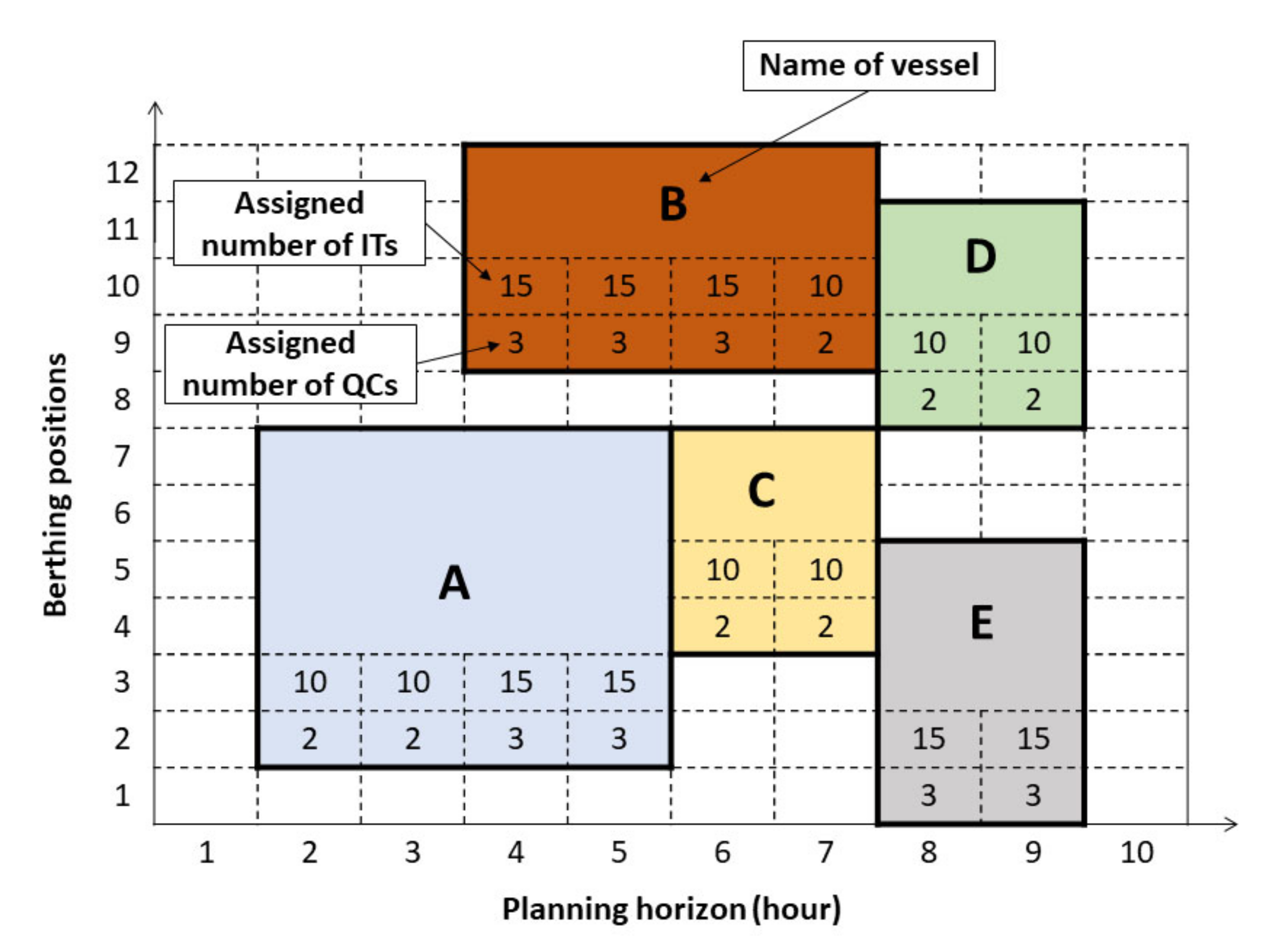
• The change in the number of QCs serving each vessel is restricted to one change at most, as was done in Reference [33]. It is worth noting that strategies for the QC assignments include time-invariant QC assignments, time-variant QC assignments, and limited time-variant QC assignments. Time-invariant QC assignments imply that the number of QCs serving each vessel must be the same during the service of the vessel [16,34], while time-variant QC assignments imply that the number of QCs can be varied dynamically according to the assignable range of QCs allowed for the vessel [12,15,17]. Note that varying the number of QCs serving the vessel is sometimes essential for improving the utilization of QCs as well as the service times of vessels. This is because some QCs serving vessels are reallocated to start operations on other vessels. However, many changes cause a long setup time, which is unacceptable in reality. Therefore, a well-balanced tradeoff is limited time-variant QC assignments, in which the variation in the number of QCs is limited. Referring to vessel B in Figure 2, it can be noted that the assigned numbers of QCs change only one time during service in time period 7. Therefore, the service duration of the vessel is divided into two stages. A stage is the number of successive time periods, and the number of QCs assigned to the vessel does not change during the same stage. A new stage starts whenever a change in the number of QCs serving the vessel occurs. Referring to Figure 2, it can be noted that vessel B has two stages. The first stage runs from time period 4 to time period 6, while the second stage starts in time period 7, in which the assigned number of QCs changes from 3 to 2;
• Minimum and maximum numbers of ITs are specified for each QC so that the waiting times of the QCs and ITs are suitable. For more details on how such numbers are determined, we refer the reader to the work of Murty et al. [20], in which the authors developed a queuing network model to capture the interactions between QCs, ITs, and yard cranes. Their model can be used to determine the numbers of ITs assigned to each QC such that that the waiting times of the QCs and ITs are minimized.

2.2.2. Notations

• SETs:
  • V: Set of arriving vessels, V= {1,2,...,n} (indexed by v);
  • T: Set of time periods in the planning horizon, T = {1,2,...,H} (indexed by t).

• Parameters:
  • $l_v$ : The length of vessel v, in which a safe distance between vessels is included;
  • $a_v$ : The time at which vessel v is expected to arrive at the terminal, called the expected arrival time;
  • $d_v$ : The time at which vessel v is expected to depart from the terminal, called the expected departure time;
  • ${\overline{b}}_v$ : The nearest berthing position to the storage yard of containers on vessel v, called the desired berthing position;
  • $L$ : The available number of berthing positions;
  • $H$ : The number of time periods in the planning horizon;
  • $Q$ : The total number of available QCs;
  • $I$ : The total number of available ITs;
  • $N_v$ : The workload of vessel v, expressed in numbers of containers in a 20-ft equivalent unit (TEU);
  • $q_v^{max}$ : Maximum number of QCs that can serve vessel v;
  • $q_v^{min}$ : Minimum number of QCs that can serve vessel v;
  • $i_{max}$ : Maximum number of ITs that can work with each quay crane;
  • $i_{min }$ : Minimum number of ITs that should work with each quay crane;
  • $R$ : Feasible range of ITs that can work with each quay crane, $R=[i_{min},i_{max}]$;
  • $c{a}_v^1$ : The penalty cost incurred if there is a deviation between the allocated berthing position, $r_v$, and ${\overline{b}}_v$ of vessel v (unit: $/unit distance deviation);
  • $c{a}_v^2$ : The energy consumption cost of vessel v per hour in idle mode (unit: $/ hour);
  • $c{a}_v^3$ : The penalty cost incurred if the departure of vessel v is later than its expected departure time (unit: $/hour);
  • $\mu$ : The average time needed to serve the ITs at the QCs;
  • 2$\tau$ : The average time needed by the ITs to travel between the quayside and the yard;
  • $\gamma$ : The average time needed to serve the ITs at the yard crane;
  • β : The berth deviation factor;
  • $M$ : A sufficiently large constant.

• Decision variables:
  • $x{b}_{jvt}$ : 1, if vessel v is berthed at berthing position j at time period t, and 0 otherwise;
  • $q_{vt}^i$ : An integer, the number of QCs serving vessel v in time period t if i ITs are assigned to each QC, i∊ R;
  • $x_{vt}$ : 1, if vessel v is processed in time period t, and 0 otherwise;
  • $g_{vt}$ : 1, if there is any decrease or increase in the number of QCs serving vessel v in time period t compared to its preceding time period (t ‒ 1), and 0 otherwise;
  • $r_v$ : Integer, the first berthing position of vessel v;
  • $S_v$ : An integer, the berthing time of vessel v;
  • $C_v$ : An integer, the completion time of vessel v, which is the largest t at which $x_{vt}$= 1 plus 1;
  • $\Delta r_v$ : An integer, the deviated distance of vessel v between the desired berthing position of vessel v and its berthing position, $\Delta r_v=\left|r_v-{\overline{b}}_v\right|$;
  • $\Delta S_v$ : An integer, the delayed berthing of vessel v, $\Delta S_v={\left(S_v-a_v\right)}^{+}$;
  • $\Delta C_v$ : An integer, the delayed departure of vessel v, $\Delta C_v={\left(C_v-d_v\right)}^{+}$;
  • $z{b}_{jvt}$ : 1, if j and t are equal to the first berthing position $\left(r_v\right)$ and berthing time $\left(S_v\right)$ of vessel v, respectively, and 0 otherwise.

2.2.3. Estimation of the Vessel Handling Time

In this section, we illustrate how to estimate the handling time of a vessel considering its assigned number of QCs and ITs. The handling time of the vessel mainly depends on the following factors:

I.

The assigned number of QCs;

II.

The assigned number of ITs serving each QC; and

III.

The distance between the vessel’s berthing position and the storage yard for the containers on the vessel.

It is worth noting that a preferred berthing position ${\overline{b}}_v$ is determined for a vessel v that is near its storage yard. If the actual berthing position of a vessel is far from its preferred position, the distances traveled by the ITs increase, and therefore, the terminal planner should employ more ITs to reduce the time the QCs wait for the ITs. Therefore, as can be seen in the work of Meisel and Bierwirth [12], if a vessel berthed$\Delta r_v$ far from its preferred berthing position, its workload is increased to $\left(1+\beta \Delta r_v\right)N_v$ TEUs. In practice, the effect of the far berthing position of the vessel can be alleviated by increasing its assigned numbers of QCs and/or ITs. Therefore, in our model, if a vessel is allocated to a berthing position far away from its preferred berthing position, its assigned numbers of QCs and/or ITs are increased. Through a simultaneous consideration of the three factors described above, the handling time for vessel v can be estimated as follows:

$$handling time=\frac{N_v·\left(1+\beta \Delta r_v\right)}{\frac{1}{\mu +2\tau +\gamma }·i·q_v^i}$$

(1)

where $q_v^i$ is the number of QCs assigned to the vessel v if i ITs are assigned to each QC. To illustrate how this formula can be used, we provide the following example, in which we assume that a vessel can be assigned three QCs simultaneously and that each QC can be assigned four ITs. We assume further that$N_v$,$\Delta r_v$, μ, τ, and γ are 300 TEUs, 10 berth segments, 0.035, 0.055, and 0.022 h, respectively. Here, $\mu +2\tau +\gamma$ designates the average time needed by an IT to transport one container from the QC serving a vessel to its storage block and to return to the QC to transport another container. Therefore, the average handling rate of one QC per one IT can be calculated by 1/($\mu +2\tau +\gamma$), expressed in containers per hour. If the berth deviation factor is 0.02, the handling time of the vessel is calculated to be approximately 5 hour, according to the above formula. Meanwhile, if$i$,$q_v^i$, and $\Delta r_v$ are changed to 2, 3, and 0, respectively, the handling time of the vessel becomes 9.2 hour. Compared to existing approaches, this proposed handling time estimation enables the consideration of the three factors simultaneously, which greatly affects the vessel handling time. This can produce a more reliable estimate of the vessel handling time, which is necessary for reliable planning. Thus, our model can improve handling plans in terms of their reliability as well as their applicability.

2.2.4. Formulation of Objective Functions

As stated before, the proposed approach considers improving the service level as well as the energy consumption of vessels, QCs, and ITs. The service level is considered through the minimization of the total delay in departure of the vessels. According to He [13], the minimization of the delayed departure of all vessels can also ensure that the energy consumption of activated QCs is minimized. This is because the shorter the delay in departure of all vessels is, the less the unproductive time of the QCs is, which can consequently improve the QCs’ energy consumption. The energy consumption of ITs mainly depends on achieving the shortest travel distance between quayside and storage yard [18]. These travel distances are highly affected by the distance from the vessel’s berthing position to the storage yards specified for its containers [10,12]. Typically, the berthing position of a vessel is optimal if it is the one closest to the storage yard areas for the containers. If the actual berthing position is far from the optimal position, the travel distances of the ITs increase. This in turn results in high congestion and more fuel consumption. Figure 3 illustrates how traffic congestion occurs when containers on vessel A are to be stored in yard 2 while containers on vessel B are to be stored in yard 1. Such traffic congestion increases the amount of fuel consumed by trucks as well as lengthening the total handling time of the vessels. Therefore, we propose a second objective function that penalizes the deviation between the desired berthing positions and the actual berthing positions of the vessels. This minimizes the energy consumption of the ITs. Finally, we use a third objective function that minimizes the waiting times of all vessels, thus minimizing the fuel consumption of vessels at port following the work of Golias et al. [11].

2.2.5. The Mathematical Model

$$\mathrm{Minimize} {\displaystyle \sum }_{v\in V}\left\{c{a}_v^1·\Delta r_v+c{a}_v^2·\Delta S_v+c{a}_v^3·\Delta C_v\right\}$$

(2)

subject to

$${\displaystyle \sum }_{v=1}^{n}x{b}_{jvt}\le 1 \forall j\in 1,\dots ,L; \forall t\in T;$$

(3)

$${\displaystyle \sum }_{v=1}^n{\displaystyle \sum }_{i=i_{min}}^{i_{max}}{q}_{vt}^i\le Q \forall t\in T;$$

(4)

$${\displaystyle \sum }_{v=1}^n{\displaystyle \sum }_{i=i_{min}}^{i_{max}}i·q_{vt}^i\le I \forall t\in T;$$

(5)

$$\frac{1}{\mu +2\tau +\gamma }{\displaystyle \sum }_{t=1}^H{\displaystyle \sum }_{i=i_{min}}^{i_{max}}i·q_{vt}^i\ge N_v·\left(1+\beta ·\Delta r_v\right) \forall v\in V;$$

(6)

$${\displaystyle \sum }_{t=1}^H{x}_{vt}=C_v-S_v \forall v\in V;$$

(7)

$$\left(t+1\right)x_{vt}\le C_v \forall v\in V;\forall t\in T;$$

(8)

$$t·x_{vt}+M\left(1-x_{vt}\right)\ge S_v \forall v\in V;\forall t\in T;$$

(9)

$${\displaystyle \sum }_{j=1}^L{\displaystyle \sum }_{t=1}^{H}z{b}_{jvt}=1 \forall v\in V;$$

(10)

$${\displaystyle \sum }_{j=1}^{j-1}{\displaystyle \sum }_{t=1}^{H}x{b}_{jvt}+{\displaystyle \sum }_{j=j+l_v}^L{\displaystyle \sum }_{t=1}^{H}x{b}_{jvt} \le M \left(1-{\displaystyle \sum }_{t=1}^{H}z{b}_{jvt}\right) \forall j=2,\dots L-l_v;\forall v\in V;$$

(11)

$${\displaystyle \sum }_{j=l_v+1}^L{\displaystyle \sum }_{t=1}^{H}x{b}_{jvt} \le M \left(1-{\displaystyle \sum }_{t=1}^{H}z{b}_{\stackrel{‘}{j}vt}\right) \forall v\in V;$$

(12)

$${\displaystyle \sum }_{j=1}^{L}x{b}_{jvt} \le M ·x_{vt} \forall t\in T;\forall v\in V;$$

(13)

$$l_v-{\displaystyle \sum }_{j=1}^{L}x{b}_{jvt} \le M \left(1-x_{vt}\right) \forall t\in T;\forall v\in V;$$

(14)

$${\displaystyle \sum }_{i=i_{min}}^{i_{max}}{q}_{vt}^i\le q_v^{max}·x_{vt} \forall t\in T;\forall v\in V;$$

(15)

$${\displaystyle \sum }_{i=i_{min}}^{i_{max}}{q}_{vt}^i\ge q_v^{min}·x_{vt} \forall t\in T;\forall v\in V;$$

(16)

$$S_v={\displaystyle \sum }_{j=1}^L{\displaystyle \sum }_{t=1}^{H}t·z{b}_{jvt} \forall v\in V;$$

(17)

$$r_v={\displaystyle \sum }_{j=1}^L{\displaystyle \sum }_{t=1}^{H}j·z{b}_{jvt} \forall v\in V;$$

(18)

$$1-\left|{\displaystyle \sum }_{i=i_{min}}^{i_{max}}{q}_{vt}^i-{\displaystyle \sum }_{i=i_{min}}^{i_{max}}{q}_{v\left(t-1\right)}^i\right|-M\left(1-g_{vt}\right)\le 0 \forall t=2,\dots ,T;\forall v\in V;$$

(19)

$$\left|{\displaystyle \sum }_{i=i_{min}}^{i_{max}}{q}_{vt}^i-{\displaystyle \sum }_{i=i_{min}}^{i_{max}}{q}_{v\left(t-1\right)}^i\right|-M·g_{vt}\le 0 \forall t=2,\dots ,T;\forall v\in V;$$

(20)

$${\displaystyle \sum }_{t=1}^H{g}_{vt}\le 3 \forall v\in V;$$

(21)

$$\Delta C_v\ge C_v-d_v \forall v\in V;$$

(22)

$$\Delta S_v\ge S_v-a_v \forall v\in V;$$

(23)

$$\Delta r_v\ge r_v-{\overline{b}}_v \forall v\in V;$$

(24)

$$\Delta r_v\ge {\overline{b}}_v-r_v \forall v\in V;$$

(25)

$$C_v\in \left\{\mathrm{1,2},\dots ,H\right\} \forall v\in V;$$

(26)

$$S_v\ge a_v \forall v\in V;$$

(27)

$$r_v\in \left\{\mathrm{1,2},\dots ,L-l_v+1\right\} \forall v\in V;$$

(28)

$$x{b}_{jvt},z{b}_{jvt}, x_{vt}, g_{vt}\in \left\{\mathrm{0,1}\right\} \forall t\in T;\forall v\in V, \forall j\in L;$$

(29)

$$\Delta C_v, \Delta S_v,\Delta r_v,q_{vt}^i\ge 0 and integer \forall v\in V.$$

(30)

The objective function of the proposed model aims to minimize the weighted sum of the penalty and energy costs of the handling operations. The objective function includes three cost parts. The first part penalizes deviating the vessel’s berthing position to somewhere distant from the storage yard for its containers. The yard implies the desired berthing position. The second part reflects the energy consumption costs if there is a time delay between the berthing and arrival times of the vessels. The third part is a penalty cost that arises if the vessel’s completion time occurs after its expected departure time. Constraint set (3) requires that in each time period, each berthing position is taken by only one vessel. Constraint sets (4) and (5) require that in each time period, the activated number of QCs and ITs do not exceed the available capacities of QCs and ITs. Constraint set (6) requires that the containers on each vessel must be entirely serviced. Constraint set (7) defines the variable$x_{vt}$ as the berthing duration and is calculated as the length of time between the berthing and completion times. This constraint also guarantees that the handling operation cannot be stopped once it begins. Constraint sets (8) and (9) describe the completion and berthing times for all vessels, respectively. Constraint set (10) ensures that within the planning horizon, each vessel must be assigned only one berthing position and one berthing time. Constraint sets (11)–(14) require that for each vessel, xb_jvt = 1 only in the grids of the time–space diagram covered by the rectangle of vessel v. The grids, which are covered by the vessel, are [S_v,…,C_v] and [r_v,…,r_v+l_v-1]. Constraint sets (15)–(16) require that the vessel’s assigned number of QCs must be within the specified boundaries. Constraint sets (17)–(18) define the variable zb_jvt. Constraint sets (19)–(20) guarantee that the number of QCs serving a vessel is adjusted at most one time during vessel service. It should be noted that the change in the assigned number of QCs can be simply adjusted using constraint set (21). For example, if the port planner prefers to set the number of crane changes to one, the right hand side of constraint set (21) is set to three. This is because there is also a change in the number of QCs at the start and end of the handling operations for the vessel. Constraint sets (22)–(25) define the variables $\Delta C_v,\Delta S_v,$and $\Delta C_{v }$respectively. Constraint set (26) guarantees that the completion time of the vessel is larger than the planning horizon boundaries. Constraint set (27) guarantees that the berthing time of each vessel is not before its arrival time. Constraint set (28) requires that the berthing position of each vessel does not exceed the berth boundaries. Constraint sets (29)–(30) are the non-negativity and binary constraints, respectively. Obviously, the proposed model is not in the standard form for mixed integer programing due to the absolute value in constraint sets (19) and (20). Therefore, the linearization instructions presented by Bertsimas and Tsitsiklis [35] were followed to remove the absolute value. By introducing the variable$l{q}_{vt}$, the mathematical model could be reduced to a mixed integer programming problem, as follows:

$$\mathrm{Minimize}{{\displaystyle \sum }}_{v\in V}\left\{c{a}_v^1·\Delta r_v+c{a}_v^2·\Delta S_v+c{a}_v^3·\Delta C_v\right\},$$

subject to constraints (3)–(18), (21)–(30), and the following constraints:

$$l{q}_{vt}\ge {\displaystyle \sum }_{i=i_{min}}^{i_{max}}{q}_{vt}^i-{\displaystyle \sum }_{i=i_{min}}^{i_{max}}{q}_{v\left(t-1\right)}^i \forall v\in V;\forall t=2,\dots ,T;$$

(31)

$$l{q}_{vt}\ge {\displaystyle \sum }_{i=i_{min}}^{i_{max}}{q}_{v\left(t-1\right)}^i-{\displaystyle \sum }_{i=i_{min}}^{i_{max}}{q}_{vt}^i \forall v\in V;\forall t=2,\dots ,T;$$

(32)

$$1-l{q}_{vt}-M\left(1-g_{vt}\right)\le 0 \forall v\in V;\forall t\in T;$$

(33)

$$l{q}_{vt}-M·g_{vt}\le 0 \forall v\in V;\forall t\in T;$$

(34)

$$l{q}_{vt}\ge 0 and integer \forall v\in V;\forall t\in T.$$

(35)

3. The Lagrangian Solution Method

As a result of combining three already complex problems, the complexity of the developed model grew dramatically. An exact solver for mixed integer programming problems is able to handle up to three vessels within one hour, while an instance of five vessels cannot be solved by the same solver. Therefore, a Lagrangian relaxation-based method was developed. The design of the Lagrangian method was motivated by the following: constraints (3), (4), and (5) make the proposed model difficult to be solved due to the limited resources for berthing positions, QCs, and ITs. Relaxing these constraints leads to a much easier problem. Therefore, a relaxed version of the problem is obtained by relaxing these constraints and adding them to the objective function with multipliers. Note that each multiplier is a penalty that is incurred in the solution when its corresponding constraint is violated. It should be noted that the solution for the relaxed problem includes a set of vessels, and each vessel has an individual cost contributing to the total solution cost. Therefore, it is possible to decompose the relaxed problem into subproblems, and each subproblem is related to only one vessel. Then, the overall solution of the problem is found by combining the solutions to the subproblems together. The optimal solution obtained by solving the relaxed problem may be infeasible due to the relaxation of the three constraints, but the optimal value can be used as a lower bound on the optimal solution of the original problem. Therefore, a feasible solution to the original problem can be generated from the solution to the relaxed problem. An optimal lower bound can be calculated by using the subgradient optimization procedures illustrated in Reference [36], which also have been considered in recent literature on the BAP, the BACAP, and the integrated QCAP and ITAP [12,30,33,37]. In these works, resource capacity constraints were dealt with as hard constraints, which if relaxed, could lead to a much easier problem that can be solved efficiently in comparison to the original problem.

3.1. The Lagrangian Relaxation for the Developed Model

In this work, Lagrangian relaxation is achieved by relaxing constraints (3), (4), and (5). The relaxed problem (P) can be written as follows:

$$\mathrm{P}:\underset{{\mathrm{xb}}_{\mathrm{jvt}},{ \mathrm{q}}_{\mathrm{vt}}^{\mathrm{i}}, \mathrm{i}·{\mathrm{q}}_{\mathrm{vt}}^{\mathrm{i}}}{\mathrm{MIN}}{{\displaystyle \sum }}_{\mathrm{V}=1}^{\mathrm{N}}\left\{{\mathrm{ca}}_{\mathrm{v}}^1·\Delta {\mathrm{r}}_{\mathrm{v}}+{\mathrm{ca}}_{\mathrm{v}}^2·\Delta {\mathrm{S}}_{\mathrm{v}}+{\mathrm{ca}}_{\mathrm{v}}^3·\Delta {\mathrm{C}}_{\mathrm{v}}\right\}+{{\displaystyle \sum }}_{\mathrm{j}=1}^{\mathrm{L}}{{\displaystyle \sum }}_{\mathrm{t}=1}^{\mathrm{H}}{\mathsf{\pi }}_{\mathrm{jt}}\left({{\displaystyle \sum }}_{\mathrm{v}=1}^{\mathrm{n}}{\mathrm{xb}}_{\mathrm{jvt}}-1\right)+{{\displaystyle \sum }}_{\mathrm{t}=1}^{\mathrm{H}}{\mathsf{\pi }}_{\mathrm{t}}\left({{\displaystyle \sum }}_{\mathrm{v}=1}^{\mathrm{n}}{{\displaystyle \sum }}_{\mathrm{i}={\mathrm{i}}_{\min }}^{{\mathrm{i}}_{\max }}{\mathrm{q}}_{\mathrm{vt}}^{\mathrm{i}}-\mathrm{Q}\right)+{{\displaystyle \sum }}_{\mathrm{t}=1}^{\mathrm{H}}{\mathsf{\pi }}_{\mathrm{t}}^{\prime }\left({{\displaystyle \sum }}_{\mathrm{v}=1}^{\mathrm{n}}{{\displaystyle \sum }}_{\mathrm{i}={\mathrm{i}}_{\min }}^{{\mathrm{i}}_{\max }}\mathrm{i}·{\mathrm{q}}_{\mathrm{vt}}^{\mathrm{i}}-\mathrm{I}\right) ,$$

(36)

subject to constraints (6)–(30) and${\pi }_{jt},{\pi }_t,{\pi }_t^{\prime }\ge 0$. Here, ${\pi }_{jt},{\pi }_t$, and${\grave{\pi }}_t$ are the Lagrangian multipliers of the relaxed constraints. By eliminating the constant parameters from (36), the relaxed problem can be written as follows:

$$P:\underset{x{b}_{jvt}, q_{vt}^i, i·q_{vt}^i}{Min}{{\displaystyle \sum }}_{v=1}^n\left\{c{a}_v^1·\Delta r_v+c{a}_v^2·\Delta S_v+c{a}_v^3·\Delta C_v\right\}+{{\displaystyle \sum }}_{j=1}^L{{\displaystyle \sum }}_{t=1}^H{{\displaystyle \sum }}_{v=1}^n{\pi }_{jt}·x{b}_{jvt}+{{\displaystyle \sum }}_{t=1}^H{{\displaystyle \sum }}_{v=1}^n{{\displaystyle \sum }}_{i=i_{min}}^{i_{max}}{\pi }_t·q_{vt}^i+{{\displaystyle \sum }}_{t=1}^H{{\displaystyle \sum }}_{v=1}^n{{\displaystyle \sum }}_{i=i_{min}}^{i_{max}}{\pi }_t^{\prime }·i·q_{vt}^i ,$$

(37)

subject to constraints (6)–(30) and ${\pi }_{jt},{\pi }_t,{\pi }_t^{\prime }\ge 0$.

The Lagrangian dual (LD) of P is as follows:

$LD:\underset{{\pi }_{jt},{\pi }_t,{\pi }_t^{\prime }}{Max}P$

$$P:\underset{x{b}_{jvt}, q_{vt}^i, i·q_{vt}^i}{Min}{{\displaystyle \sum }}_{v=1}^n\left\{c{a}_v^1·\Delta r_v+c{a}_v^2·\Delta S_v+c{a}_v^3·\Delta C_v\right\}+{{\displaystyle \sum }}_{j=1}^L{{\displaystyle \sum }}_{t=1}^H{{\displaystyle \sum }}_{v=1}^n{\pi }_{jt}·x{b}_{jvt}+{{\displaystyle \sum }}_{t=1}^H{{\displaystyle \sum }}_{v=1}^n{{\displaystyle \sum }}_{i=i_{min}}^{i_{max}}{\pi }_t·q_{vt}^i+{{\displaystyle \sum }}_{t=1}^H{{\displaystyle \sum }}_{v=1}^n{{\displaystyle \sum }}_{i=i_{min}}^{i_{max}}{\pi }_t^{\prime }·i·q_{vt}^i ,$$

(38)

subject to constraints (6)–(30) and ${\pi }_{jt},{\pi }_t,{\pi }_t^{\prime }\ge 0$.

To obtain the Lagrangian dual (LD_v) for the subproblem P_v, P is decomposed into a set of subproblems, each of which represents a vessel. LD_v is as follows:

$L{D}_v:\underset{{\pi }_{jt},{\pi }_t,{\pi }_t^{\prime }}{Max}{P}_v$

$$P_v:\underset{x{b}_{jvt}, q_{vt}^i, i·q_{vt}^i}{Min}\left\{c{a}_v^1·\Delta r_v+c{a}_v^2·\Delta S_v+c{a}_v^3·\Delta C_v\right\}+{{\displaystyle \sum }}_{j=1}^L{{\displaystyle \sum }}_{t=1}^H{\pi }_{jt}·x{b}_{jvt}+{{\displaystyle \sum }}_{t=1}^H{{\displaystyle \sum }}_{i=i_{min}}^{i_{max}}{\pi }_t·q_{vt}^i+{{\displaystyle \sum }}_{t=1}^H{{\displaystyle \sum }}_{i=i_{min}}^{i_{max}}{\pi }_t^{\prime }·i·q_{vt}^i ,$$

(39)

subject to constraints (6)–(30) and ${\pi }_{jt},{\pi }_t,{\pi }_t^{\prime }\ge 0$.

3.2. The Overall Procedures for the Subgradient Optimization Method

The overall procedures described in the work of Geoffrion [36] are as follows:

Step 1: 

Initialize the upper bound (Z_UB) as a large value and the multipliers ${\pi }_{jt},{\pi }_t,$and${\pi }_t^{\prime }$ as 0.

Step 2: 

The lower and upper bounds of the optimal solution objective are calculated as follows:

• Step 2.2: For each vessel v, solve LD_v using initial values of the multipliers. The procedures for solving LD_v will be presented in Section 3.3. The lower bound of the solution objective (Z_LB) is formed by (34), and the largest lower bound is updated,$Z_{LB}^{max}=\max \left(Z_{LB}^{max},Z_{LB}\right)$.
• Step 2.3: If the solution obtained using (36) violates the relaxed constraints, a feasibility restoration method is used to solve the infeasibilities and calculate the upper bound (Z_UB). Afterwards, update the lowest upper bound,$Z_{UB}^{min}=\max \left(Z_{UB}^{min},Z_{UB}\right)$.

Step 3: 

Evaluate the subgradients as well as the step sizes to calculate the multipliers ${\pi }_{jt},{\pi }_t,$and${\pi }_t^{\prime }$.

The subgradients $G_{jt},G_t, \mathrm{and} G_t^{\prime }$ can be calculated as follows:

$$G_{jt}={\displaystyle \sum }_{v=1}^{n}x{b}_{jvt}-1 \forall j=1,\dots ,L;t\in T;$$

(40)

$$G_t={\displaystyle \sum }_{v=1}^n{\displaystyle \sum }_{i=i_{min}}^{i_{max}}{q}_{vt}^i-Q \forall t\in T;$$

(41)

$$G_t^{\prime }={\displaystyle \sum }_{v=1}^n{\displaystyle \sum }_{i=i_{min}}^{i_{max}}{q}_{vt}^i-Q \forall t\in T.$$

(42)

The step sizes can be calculated as follows:

$${\alpha }_1=\frac{\lambda \left(Z_{UB}-Z_{lB}\right)}{{{\displaystyle \sum }}_{j=1}^L{{\displaystyle \sum }}_{t=1}^H{G}_{jt}^2};$$

(43)

$${\alpha }_2=\frac{\lambda \left(Z_{UB}-Z_{lB}\right)}{{{\displaystyle \sum }}_{t=1}^H{G}_t^2};$$

(44)

$${\alpha }_3=\frac{\lambda \left(Z_{UB}-Z_{lB}\right)}{{{\displaystyle \sum }}_{t=1}^H{G}_t^{\prime 2}};$$

(45)

where $\mathit{\lambda }$ is a variable for adjusting the step sizes; and $\mathit{\lambda }$ has a value in the range from 0 to 2. In the first iteration of the procedures, $\mathit{\lambda }$is initialized to 2 and is halved as long as there is no improvement in the lowest upper bound ($Z_{UB}^{min}$) for a specified number of successive iterations. The procedure is aborted if $\mathit{\lambda }$reaches a value below 0.005 or the duality gap between$Z_{UB}^{min}$ and $Z_{LB}^{max}$ is below one.

Step 4: 

The multipliers ${\pi }_{jt},{\pi }_t,$and${\pi }_t^{\prime }$, for the next iteration, are calculated as follows:

$${\pi }_{jt}=\max \left(0,{\pi }_{jt}+{\alpha }_1·G_{jt}\right) \forall j=1,\dots ,L;\forall t\in T;$$

(46)

$${\pi }_t=\max \left(0,{\pi }_t+{\alpha }_2·G_t\right) \forall t\in T;$$

(47)

$${\pi }_t^{\prime }=\max \left(0,{\pi }_t^{\prime }+{\alpha }_3·G_t^{\prime }\right) \forall t\in T.$$

(48)

Step 5: 

Return to step 2.

3.3. The Overall Procedures for the Subgradient Optimization Method

The following section presents the proposed systematic procedures for obtaining solutions to the decomposed primal problem (LD_v) for vessel v. The solution for LD_v describes the berthing position, berthing time, QC assignments, IT assignments, and completion time for vessel v. Before introducing the detailed steps of the systematic procedures, an example is provided to illustrate some terms to be used in the explanation. Consider vessel A, which has $N_A$= 400, $q_A^{max}$= 4, $l_A$= 5, $a_A$= 3, and ${\overline{b}}_A$= 4. Furthermore, the terminal data are as follows: $i_{max}$= 5, $H$= 8, and $L$= 9. As shown before, the vessel is represented in the space–time diagram by a rectangle. Now, it is required to represent the feasible region within which the left lower vertex (or reference corner) of the vessel’s rectangle can be located. Figure 4 shows the feasible region of vessel A, which is shaded in gray. The feasible region is determined through its respective spatial and temporal constraints. The symbol w_A in Figure 4 represents the longest time period during which vessel A can be berthed and is calculated as the rounded (up) value of $H-\frac{N_A}{pr\ast i_{max}\ast q_A^{max}}+1$, where $pr=\frac{1}{\mu +2\tau +\gamma }$. Moreover, the time–space diagram can be divided into grids, and each grid can be described by$\left(j,t\right)$. It can also be noted that (${\overline{b}}_A,a_A)$ represents the perfect location of the left lower vertex of the vessel rectangle, as the berthing cost (the sum of the second and third terms of the objective function) is zero. However, when the container terminal is congested, the reference corners of some vessels’ rectangles deviate from their ideal locations due to the limited availability of berthing positions, QCs, and ITs.

The proposed procedures first determine the lowest cost in terms of berthing time and berthing position. Then, assignments of QCs and ITs are generated for the identified berthing position and time. After that, the objective function in (39) is calculated for the current schedule (berthing time, berthing position, completion time, and assignments of QCs and ITs).

The procedures, from step 1 to step 3, are performed for all feasible combinations of $\left(j,t\right)$ at which the reference corner of vessel v can be located, where $j=1,\dots ,L-l_v+1$ and $t=a_v,\dots ,H-\frac{N_v}{pr\ast i_{max}\ast q_v^{max}}+1$.

Step 1: 

Assign an initial value to the minimum objective value, e.g., 15,000, and set j = 1 and t = 1.

Step 2: 

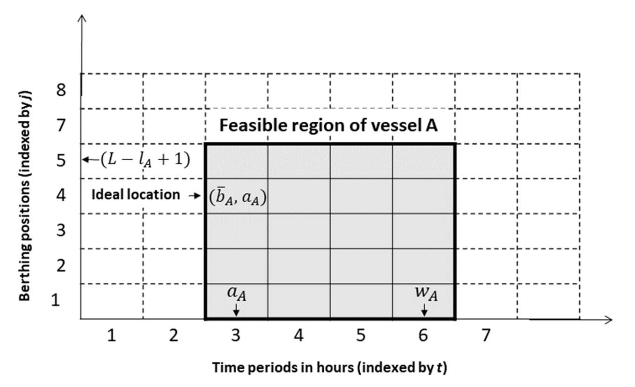
This step aims to determine the coordinates of the left lower corner (reference corner) of the vessel rectangle in the time–space diagram, i.e., $r_v$and $S_v$. The minimum value of the berthing cost ($c{a}_1·\Delta r_v+c{a}_2·\Delta S_v+{\displaystyle \sum }_{j=1}^L{\displaystyle \sum }_{t=1}^H{\pi }_{jt}·x{b}_{jvt})$is used to decide on the best values of $r_v$ and $S_v$. Note that if $r_v$ and $S_v$ are searched for in each grid in the feasible region, this would increase the computational time. Therefore, instead of trying all grids in the feasible region, $r_v$ and $S_v$ are searched for in the grids around (${\overline{b}}_v,a_v)$ because the optimal values of $r_{v }$and $S_v$ may be close or equal to ${\overline{b}}_v$ and $a_v$, respectively. For this, $r_v$ and $S_v$ are searched for time period by time period, starting from$a_v \mathrm{to} \left(H-\frac{N_v}{pr\ast i_{max}\ast q_v^{max}}+1\right).$ At each time period, the following steps are performed.

Step 2.1: 

Select the next grid, starting from ${\overline{b}}_v$ through$L-l_v+1$. If the berthing cost in the grid is lower than the minimum objective value, go to step 3. Otherwise, go back to the beginning of step 2.1 until all berthing positions from${\overline{b}}_v$through $L-l_v+1$are tried once, and then go to step 2.2. It is important to point out that the minimum objective value is iteratively updated in step 3 based on the vessel schedule (berthing time, berthing position, completion time, and assignments of QCs and ITs). Therefore, if the berthing cost is higher than the minimum objective value, this implies that berthing the vessel in the grid corresponding to this berthing cost will not yield an objective value better than the current minimum objective value. Therefore, this grid is excluded, and the next grid is tried. In this way, step 3 is not performed for all the grids in the feasible region, and thus computational time can be saved.

Step 2.2: 

Select the next grid, starting from$({\overline{b}}_v-1$) to 1. If the berthing cost in the grid is lower than the minimum objective value, go to step 3. Otherwise, go back to the beginning of step 2.2 until all berthing positions from$\left({\overline{b}}_v-1\right)$ to 1 are tried once, and then go to step 2.

Step 3: 

The reference corner of the rectangle corresponding to vessel v is located at (j,t), which is determined by step 2. Hereafter, in this step, the QCs and ITs are allocated to vessel v. To stimulate limited time-variant quay crane assignments, the service of the vessel is divided into two stages. The first and second stages are designated by $t_1$ and$t_2$, respectively. To try all feasible combinations of the QCs and ITs that can be allocated to vessel v, the following steps are performed.

Step 3.1: 

If all combinations of ($q_1$, $i_1$),$q_1=q_v^{min},\dots ,q_v^{max}$, and $i_1=i_{min},\dots ,i_{max}$ are tried once, go back to step 2. Otherwise, select the next combination of ($q_1$, $i_1$) and set $t_1$= 1, where $t_1$ is the first stage at which $q_1$ QCs are assigned to vessel v and $i_1$ ITs are assigned to each QC.

Step 3.2: 

For all combinations of ($q_2$, $i_2$),$q_2=q_v^{min},\dots ,q_v^{max}$, and $i_2=i_{min},\dots ,i_{max}$, select the next combination of ($q_2$,$i_2$) and set $t_2$ to the rounded value of max $\left\{0,\frac{N_v-(pr\ast i_1\ast q_1)\ast t_1}{(pr\ast i_2\ast q_2)}\right\}$, where $t_2$ is the second stage at which vessel v is assigned $q_2$ QCs and $i_2$ ITs are assigned to each QC so as to completely handle $N_v$. If t + t₁ + t₂ - 1 ≤ H, then obtain the objective value of (39) corresponding to the schedule just identified for the combination of {j, t, t₁, q₁, i₁, t₂, q₂, i₂}, and update the minimum objective value. If two or more schedules have the minimum objective value, random selection is used to select the vessel’s schedule from these schedules. Otherwise, go to step 3.2 until all combinations ($q_2$, $i_2$) have been tried once.

Step 3.3: 

If $t_1\le \frac{N_v}{pr\ast i_1\ast q_1}$, increase t₁ by one and go to step 3.2. Otherwise, go to step 3.1.

The lowest objective value determined from step 3.2 represents the best solution for LD_v. Equation (36) is used to obtain the lower bound of the optimal solution objective. It should be noted that the obtained solution may violate the relaxed constraints; therefore, the solution may be infeasible. In this case, another method is utilized to make the solution feasible.

3.4. Feasibility Restoration and Solution Refinement

As stated before, it may happen that some iterations of the subgradient method find an infeasible solution. In this case, the following procedures are used to change the infeasible solution into a feasible solution.

Step 1: 

Sort vessels sequentially in increasing orders of$a_v$ and set v = 0 and Fe = In = ∅, where Fe and In are feasible and infeasible sets, respectively.

Step 2: 

Increase v by 1 and perform step 2 if v ≤ n. Otherwise, go to step 3. In this step, the obtained solution of the vth vessel is checked for any violation of the relaxed constraints, given that the solutions for the preceding vessels in Fe are known. If there is no violation of the relaxed constraints, the vth vessel is inserted into Fe. Otherwise, the vth vessel is inserted into In. Return the beginning of this step.

Step 3: 

Sort vessels in In sequentially in increasing orders of$a_v$, and then the next vessel in In is selected. The procedures in Section 3.3 are used to find the least-cost feasible schedule for the selected vessel that results in no violation of the relaxed constraints, provided that the solutions of vessels in Fe are given. Afterwards, the selected vessel is deleted from In and is inserted into Fe. Redo step 3 until In contains no vessels.

Step 4: 

After a feasible solution is constructed by performing the previous steps, the feasible solution is refined. As noted, the solution is composed of a set of vessels. Each vessel has its own cost that contributes to the overall quality of the obtained solution. Therefore, if the schedules of vessels with relatively higher costs are refined, the overall solution cost may be improved. A straightforward procedure is applied as follows: Sort vessels sequentially in decreasing order of their individual cost. For the first 20% of vessels at the top of the list, perform the same procedure of solving the decomposed primal problems. It is important to point out that a percentage of 20% is selected because if this percentage were higher, more vessels will have to carry out the procedure of solving, which would lead to an increased computational time.

3.5. An Illustrative Example

To illustrate the proposed heuristic algorithm, the results of some iterations during solving a numerical example of the three vessels A, B, and C are provided in Figure 5. In this numerical example, the number of available QCs and ITs is set to 8 and 35, respectively. Moreover, the minimum and maximum limits of the ITs are 3 and 5, respectively. This implies that there is a shortage of five ITs, such that it is impossible to provide each QC with its maximum number of ITs when all of the available QCs are activated.

Figure 5a illustrates the first iteration of the developed subgradient optimization method when all multipliers have values of zero. Note that in the first iteration, each vessel is berthed at its ideal location, (${\overline{b}}_A,a_A)$. As can be seen in Figure 5a, there is a violation of the crane capacity constraint (4) as well as the truck capacity constraint (5). The violation is indicated in red in Figure 5a. In addition, the rectangles overlap with each other. This means that constraint (3) is also violated. During the iterative procedure of the subgradient optimization, the multipliers corresponding to the grids, in which constraints (3), (4), and (5) are violated, increase. The objective function value of LD_v in (39) is a function of the multipliers. Therefore, the objective function value belonging to the vessels, which are berthed in these grids, increases, leading to a reallocation of berthing positions, berthing times, QCs, and ITs to these vessels. The results, with updated multipliers, are shown in Figure 5b,c, in which it can be noted that violations of constraints (3), (4), and (5) are reduced compared to the first iteration in Figure 5a. Figure 5d shows the final solution for the numerical example.

4. Numerical Experiments

This section includes four parts. The first part shows how test instances are generated. In the second part, a number of small test instances are solved using the developed Lagrangian method, and the results are validated against the results produced by the ILOG CPLEX^TM solver. Numerical experiments with large problem sizes are carried out in the third part. In the fourth part, we illustrate the added value of the proposed approach using a comparison to an existing approach. All of the experiments were carried out using a computer with a 2.5-GHz processor and 1 GB of RAM. The Lagrangian method was coded on MATLABTM.

4.1. Generating Test Instances

To generate realistic instances for a performance assessment of the developed Lagrangian method, three vessel classes, i.e., feeder, medium, and jumbo, were created, as in Reference [12]. The vessel classes have different technical characteristics, as illustrated in

Table 1. Technical characteristics of the different vessel classes.

Class	${\mathit{l}}_{\mathit{v}}^{*}$	${\mathit{N}}_{\mathit{v}}$	${\mathit{q}}_{\mathit{v}}^{\mathit{m}\mathit{i}\mathit{n}}$	${\mathit{q}}_{\mathit{v}}^{\mathit{m}\mathit{a}\mathit{x}}$
Feeder	U (3, 4) + 1**	U (150, 450)	1	2
Medium	U (4, 6) + 1	U (450, 1400)	2	4
Jumbo	U (6, 7) + 1	U (1400, 1900)	4	6

* $l_v$ is expressed in units of 50 m. ** U represents a uniform distribution.

. In each generated instance, feeders represent 60% of the vessels, medium vessels represent 30% of the vessels, and jumbo vessels represent 10% of the vessels. The planning horizon’s length is set to one week and is discretized into one-hour periods. The quay length is assumed to be 1000 m and is partitioned into 50-meter segments. Thus, the available number of berthing times (H) and berthing positions (L) is 168 and 20, respectively. The expected arrival times, the preferred berthing positions, and the expected departure times are generated from$U\left(\mathrm{1,168}\right)$, $U\left(1,L-l_v+1\right),$ and the rounded value of $a_v+N_v/\left(30\ast q_v^{max}\right)+U\left(\mathrm{5,10}\right)$, respectively. The remaining model parameters are as follows: $Q$ = 10,$I$ = 40, $i_{max}$ = 5, $i_{min}$ = 3, and $\beta$ = 0.01. Moreover, $\mu ,\tau$, and $\gamma$ are 0.035, 0.055, and 0.022 hour, respectively. Finally,$c{a}_v^1$, $c{a}_v^2$, and $c{a}_v^3$ were estimated to be $1000/unit distance deviation, $1000/hour, and $1000/hour, respectively. However, the developed model can be solved using different weight values. It should be noted that different values of$c{a}_v^1$, $c{a}_v^2$, and $c{a}_v^3$ will clearly influence the results. For example, decreasing $c{a}_v^1$ will result in allowing vessels to be moored at any available berthing position along the quay. This in turn increases the deviation between the expected and actual berthing positions, and thus, more energy is consumed by ITs traveling between the quay side and storage areas. It is worth noting that larger value of $c{a}_v^1$ is preferred for large container terminals. This is because the travel distance between the quay side and the storage areas is significant in large container terminals compared to small ones. Setting the value of $c{a}_v^2$ to be higher than$c{a}_v^1$ and $c{a}_v^3$ will force the model to decrease emissions from vessels by minimizing their waiting times at the terminal. This means that large value of $c{a}_v^2$ allows for serving vessels almost on a first-come, first-served basis. Large values of $c{a}_v^2$ are preferred for container terminals serving vessels whose idle emissions are relatively high, such as vessels whose workload is mostly refrigerated containers. Setting the value of $c{a}_v^3$ higher than $c{a}_v^1$ and $c{a}_v^2$ will ensure that most vessels depart from the terminal according to their promised departure times. This suits container terminals whose handling equipment is energy-efficient, and thus, such terminals pay more attention to improving service levels by using large values of$c{a}_v^3$. Future research should focus on more detailed analyses of $c{a}_v^1$, $c{a}_v^2$, and $c{a}_v^3$. Here, equal values are used to illustrate the proposed methodology.

4.2. Comparison to Cplex Results

To judge the quality of the solutions found using the developed Lagrangian method, the solutions determined by the developed method were compared to the optimal solutions obtained from solving the proposed model using ILOG CPLEX^TM (IBM, New York, NY, USA). For instances of small sizes, the optimal solutions were found by CPLEX in short computational times. However, the computational time became relatively long with increasing instance sizes, and in some cases, it was not possible to find the optimal solution due the limited physical memory of the PC. Consequently, this section presents the solutions of small size instances. Note that each instance was solved 10 times using the Lagrangian method, and the average upper and lower bounds for each instance were calculated. The computational results for the comparison are given in

Table 2. Comparison to CPLEX results.

Instance # (No. of Vessels)		CPLEX			The Heuristic Algorithm
					The Average Values
	Optimal Solution	Lower Bound	CPU*(min.)	Upper Bound (UB)	Lower Bound (LB)	CPU (min.)	$\mathbf{Gap} \%=\frac{\mathit{U}\mathit{B}-\mathit{L}\mathit{B}}{\mathit{U}\mathit{B}}\times 100$
1(3)	4000	-	2.24	4000	3510	0.5236	12.2
2(4)	3000	-	5.43	3000	2307.5	0.791310	23.08
3(4)	2000	-	19.27	2000	1112.1	0.616287	44.39
4(4)	4000	-	6.54	4000	3902.2	0.895599	2.45
5(4)	2000	-	0.23	2000	2000	0.031226	0
6(4)	3000	-	15.54	3000	2886.6	0.505049	3.78
7(4)	4000	-	4.15	4000	3790	1.118004	5.25
8(5)	7000	-	20.13	7000	6234.7	1.51	10.93
9a(5)	-	5771.12	39.89	8000	7634.91	2.01	4.56
10a(5)	-	-	13.56	8000	7512	2.384742	6.10
11a(5)	-	-	42.32	9000	8464.4	1.085400	5.95

^a CPLEX stopped due to being out of memory. * CPU time is the processing time in minutes.

. In these experiments, the planning horizon was 24 hour (one day). It is worth noting that the average upper bound represents the feasible objective value (final solution) that could be found using the Lagrangian method. As shown in Table 2, the Lagrangian method could find the optimal solutions for the instances that could be solved to optimality by solving the proposed mixed integer programming model using ILOG CPLEX^TM.

To judge the quality of the lower bounds found using the Lagrangian method, the lower bounds found using the proposed procedures to solve the decomposed primal problems (Section 3.3) were compared to the optimal solutions found by ILOG CPLEX^TM. The results illustrate that the lower bounds found using the Lagrangian method are lower than the optimal solutions found by ILOG CPLEX^TM in all instances. This implies that the procedures for solving the decomposed primal problems can produce optimal lower bounds, and thus the relative gap “Gap %” between the average upper bound and average lower bound can be used as a measure of the performance of the developed algorithm.

4.3. Solving Instances with Large Sizes

To check the performance of the developed Lagrangian method in solving generated instances of a realistic size, three sets of instances, including 20, 25, and 30 vessels, were randomly generated. Each set contained 10 instances. The numerical experiments for the differently sized instances can be seen in

Table 3. The computational results of the differently sized instances.

Instance # (Size)	The Worst			The Best			The Average
	LB*	UB*	Gap %	LB	UB	Gap%	LB	UB	CPU (Min.)	Gap %
1 (20)	25.39	27	5.97	25.99	26	0.03	25.64	26.4	10.14	2.89
2 (20)	28.46	31	8.19	28.86	29	0.49	28.7	29.8	10.84	3.7
3 (20)	8.16	9	9.29	8.55	9	5.01	8.38	9	4.26	6.87
4 (20)	24.3	27	10.01	24.45	27	9.44	24.34	27	6.08	9.83
5 (20)	17.93	23	22.05	18.36	21	12.59	18.15	22	5.82	17.5
6 (20)	29.37	40	26.58	30.19	33	8.52	29.95	37.6	9.1	20.36
7 (20)	22.71	27	15.89	22.9	23	0.45	22.82	24	21.5	4.93
8 (20)	24.11	28	13.89	24.64	26	5.25	24.35	27	10.2	9.8
9 (20)	18.63	23	19	19.72	21	6.1	19.22	22	4.8	12.65
10 (20)	23.14	24	3.6	23.91	24	0.38	23.6	24	5.22	1.66
11 (25)	32.3	40	19.24	32.69	37	11.64	32.45	38.4	16.57	15.5
12 (25)	34.12	43	20.64	34.56	36	4	34.27	38.6	14.86	11.23
13 (25)	42.77	62	31.02	42.95	51	15.79	42.85	58.8	14.74	27.13
14 (25)	21.82	30	27.28	21.86	24	8.9	21.83	25.4	6.02	14.04
15 (25)	35.77	43	16.82	36.11	41	11.93	35.91	41.4	15.92	13.26
16 (25)	19.39	22	11.86	20.09	21	4.35	19.82	21.6	7.12	8.22
17 (25)	34.71	36	3.58	34.94	35	0.19	34.8	35.4	8.5	1.69
18 (25)	30.41	38	19.98	30.75	34	9.57	30.59	35.8	14.86	14.55
19 (25)	25.8	31	16.78	26	26	0	25.92	27.4	7.28	5.41
20 (25)	44.02	67	34.3	44.24	51	13.3	44.09	55.4	17.65	20.4
21 (30)	41.1	49	16.13	41.96	44	4.65	41.52	46.2	12.64	10.13
22 (30)	43.46	75	42.05	43.68	59	25.96	43.59	67.8	37.15	35.71
23 (30)	44.18	51	13.37	44.18	47	5.99	44.18	49.8	9.46	11.28
24 (30)	42.74	65	34.2	42.94	53	19.0	42.84	58.4	46.15	26.6
25 (30)	32.24	60	46.26	32.67	49	33.32	32.46	54.6	29.17	40.56
26 (30)	50.4	59	14.58	51.5	52	0.96	51.02	56.2	22.64	9.22
27 (30)	61.23	69	11.26	61.8	64	3.44	61.51	67.8	31.55	9.28
28 (30)	44.48	61	27.08	45.9	51	9.99	45.18	59.8	22.46	24.44
29 (30)	45.99	74	37.86	45.88	68	32.53	45.03	71.8	46.15	37.34
30 (30)	42.99	75	42.69	41.91	71	40.97	42.06	74.6	29.17	41.62
Average	33.07	43.63	20.72	33.47	38.43	10.16	33.24	41.13	16.60	15.66

* UB and LB represent the upper bound and lower bound, respectively, expressed in units of $1000.

. The worst, best, and average values of the upper bounds, lower bounds, and gaps, as well as the average computational time (obtained after running the method 10 times), are shown in Table 3. As can be noted from Table 3, the gap and the computational time increased as the problem size increased. On average, the gap and computational time were 15.66% and 16.66 min, respectively. However, we can observe that the average gap and average computational time were more than 30% and more than 40 min, respectively, for some instances of 30 vessels. This is because the higher the number of vessels is, the more the degree of overlap between the vessels becomes significant. This makes such instances difficult to be solved with limited numbers of berthing positions, QCs, and ITs. Thus, during the iterative procedure for the subgradient optimization, the multipliers related to the grids, where the vessels overlapped with each other, were increased. This led to moving the overlapping vessels to unallocated grids away from their ideal locations, resulting in an increase in the objective value for some vessels: to try more grids in the feasible region and in each grid, steps 3.1 to 3.3 are performed, which increases the computational time.

In Table 3, it can also be observed that the average statistics (in the last rows of the table) for the upper and lower bounds for the worst, best, and average cases were slightly different. This implies that in terms of consistency, the efficiency of the proposed method is fairly high.

Figure 6a shows the lower bound and the corresponding upper bound generated during the iterative procedure for instance 14. The convergence of the heuristic for instance 14 is also presented in Figure 6b. The upper and lower bounds converged after 56 iterations, resulting in a solution of 24,000 with an optimality gap of 16.67%.

The performance of the developed Lagrangian method was considered to be satisfactory in solving the realistically sized instances, considering the increasing difficulty of the research problem as the problem size increase. Moreover, it should be noted that we solved these instances with a shortage in trucks, which also increases the problem difficulty.

4.4. Significance of the Proposed New Integration Framework

In this section, we demonstrate the significance of the proposed integration framework for the BAP, QCAP, and ITAP by comparing our approach to an existing approach. We solved an instance by using our approach and the approach of Ursavas [17] with different numbers of ITs. The main reason for specifically choosing the approach of Ursavas [17] is that she considered QCs with different handling rates, which facilitated a comparison to our approach, as will be illustrated later. In the following section, we refer to the approach of Ursavas [17] as the existing approach. To compare the two approaches to each other, we modified the objective function of the existing approach to be the same as our objective function. In order to solve the instance with different numbers of ITs using the existing approach, the handling rates of the QCs were reduced according to the truck shortage, as follows: 30 TEUs/h for a QC with five ITs, 24 TEUs/h for a QC with four ITs, and 18 TEUs/h for a QC with three ITs. For example, if the truck capacity was reduced from 50 to 45, then five QCs would have a handling rate of 24 TEUs/h because these five QCs would be assigned four ITs instead of five ITs, while the remaining QCs would be assigned five ITs and would work with a handling rate of 30 TEUs/h. Figure 7 shows the total handling costs obtained using the two approaches for this instance if the number of ITs varied from 40 to 50 and all other parameters were held constant. The two approaches could obtain a total handling cost of $30,000 with no shortage in trucks (I = 50). It can be observed that compared to our approach, the handling costs found by the existing approach obviously increase with decreasing numbers of available ITs. Interestingly, in some cases, e.g., I = 45, 44, and 43, the handling costs obtained using our approach are the same, while the handling costs obtained using the existing approach increase with decreasing available ITs. The main reason is that our proposed approach can handle the shortage in ITs such that this shortage does not affect the handling cost of the vessels, as illustrated in detail in Section 2.1. On average, our approach could improve the solutions for the instances with different numbers of ITs by 6% compared to the solutions obtained using the existing approach. This ensures that the integration of the BAP, QCAP, and ITAP has a significant added value for container terminals. In addition, integrating the BAP, QCAP, and ITAP leads to a more reliable estimation of vessel handling times, and therefore, such integration is an essential factor in managing handling operations in container terminals.

5. Conclusions

The operational efficiency of container terminals (e.g., short service times and low operating costs) is highly dependent on effective planning of the handling operations of vessels using the available berths, QCs, and ITs, which are scarce and expensive resources. Because significant overhead costs for container terminals are also caused by energy consumption, it is essential to reduce energy consumption to achieve cost reduction and higher profits. Therefore, recent studies have considered the tradeoff between energy-saving objectives and time-saving objectives in planning handling operations for container terminals.

This paper presented a mixed integer programming model for integrating the BAP, the QCAP, and the ITAP, considering energy-saving goals. As a result of integrating three already complex problems, the complexity of the resulting model increased dramatically, and therefore, there was a need for an efficient solution method. Thus, a Lagrangian relaxation-based method was developed to solve the model.

The main contribution of the presented model is the integration of the BAP, the QCAP, and the ITAP, considering the energy-saving goals of vessels, QCs, and ITs. In addition, we estimate the vessel handling time considering the number of QCs assigned to the vessel, the number of ITs assigned to each QC, and the distance between the berthing position of the vessel and its storage yard. Therefore, compared to the traditional BACAP, the integrated model yields better estimates of vessel handling times and enables reduction in energy costs. Furthermore, rather than renting external trucks to compensate for the lack of ITs as suggested by existing studies, which would increase the operating and energy costs of the handling plan, the integrated model can handle the limited availability of ITs and provides a handling plan with a lower cost than what would be obtained by solving these problems separately.

Numerical experiments were carried out to assess the performance of the developed Lagrangian method. The solutions of the developed method were validated against those found by an exact solver. The exact solver failed to reach an optimal solution or a lower bound for instances of a practical size, while the developed method could obtain an upper bound and a lower bound for all test instances. This reflects the benefits of developing a heuristic solution method for instances with a large size to provide a good solution within a practical amount of time. The developed method could obtain near optimal solutions with an average gap of 15.66% and an average computational time of 16.60 min.

In addition, the results showed that compared to the existing approach, the solutions obtained by our approach in the case of a shortage of ITs caused no delay in the service of the vessels. The idea is that the proposed new model reallocates the QCs and ITs to vessels in a way that the available capacities of the QCs and ITs are not violated. This enables the production of better solutions in the case of a limited availability of ITs, and this therefore confirms the need to integrate the BAP, QCAP, and ITAP, as proposed in this work.

In future research, the developed model can be extended to determine the assignment of QCs to each specific vessel. In the current work, the solution time was a bit consuming. Therefore, other heuristic and metaheuristic approaches can be investigated to improve the solution time of the proposed problem. Finally, future work may address the possibility of alternative fuels for IT and QC engines/motors, or autonomous vehicles that would reduce labor costs and limitations in terms of drivers. All of these proposals could save on costs and emissions.

References

1. Juan, W.; Asariotis, R.; Assaf, M.; Ayala, G.; Benamara, H.; Chantrel, D.; Hoffmann, J.; Premti, A.; Rodríguez, L.; Youssef, F. Review of Maritime Transport; UNCTAD: New York, NY, USA, 2019; ISBN 978-92-1-112958-8. [Google Scholar]
2. Cao, J.; Shi, Q.; Lee, D.-H. Integrated Quay Crane and Yard Truck Schedule Problem in Container Terminals. Tsinghua Sci. Technol. 2010, 15, 467–474. [Google Scholar] [CrossRef]
3. He, J.; Huang, Y.; Yan, W.; Wang, S. Integrated internal truck, yard crane and quay crane scheduling in a container terminal considering energy consumption. Expert Syst. Appl. 2015, 42, 2464–2487. [Google Scholar] [CrossRef]
4. He, J.; Zhang, W.; Huang, Y.; Yan, W. A simulation optimization method for internal trucks sharing assignment among multiple container terminals. Adv. Eng. Inform. 2013, 27, 598–614. [Google Scholar] [CrossRef]
5. Bierwirth, C.; Meisel, F. A follow-up survey of berth allocation and quay crane scheduling problems in container terminals. Eur. J. Oper. Res. 2015, 244, 1–15. [Google Scholar] [CrossRef]
6. Carlo, H.J.; Vis, I.F.A.; Jan, K. Transport operations in container terminals: Literature overview, trends, research directions and classification scheme. Eur. J. Oper. Res. 2014, 236, 675–689. [Google Scholar] [CrossRef]
7. Lee, D.; Qiu, H.; Miao, L. Quay crane scheduling with non-interference constraints in port container terminals. Transp. Res. Part E Logist. Transp. Rev. 2008, 44, 124–135. [Google Scholar] [CrossRef]
8. Acciaro, M.; Vanelslander, T.; Sys, C.; Ferrari, C.; Roumboutsos, A.; Giuliano, G.; Lam, J.S.L.; Kapros, S. Environmental sustainability in seaports: A framework for successful innovation. Marit. Policy Manag. 2014, 41, 480–500. [Google Scholar] [CrossRef]
9. Huang, G.Q.; Pratap, S.; Zhang, M.; Shen, C.L.D. A multi-objective approach to analyse the effect of fuel consumption on ship routing and scheduling problem. Int. J. Shipp. Transp. Logist. 2019, 11, 161. [Google Scholar] [CrossRef]
10. Abdel-Fattah, A.; El-Tawil, A.; Harraz, N. An Integrated Operational Research and System Dynamics Approach for Planning Decisions in Container Terminals. Int. J. Ind. Sci. Eng. 2013, 7, 273–279. [Google Scholar]
11. Golias, M.M.; Saharidis, G.K.; Boile, M.; Theofanis, S.; Ierapetritou, M.G. The berth allocation problem: Optimizing vessel arrival time. Marit. Econ. Logist. 2009, 11, 358–377. [Google Scholar] [CrossRef]
12. Meisel, F.; Bierwirth, C. Heuristics for the integration of crane productivity in the berth allocation problem. Transp. Res. Part E Logist. Transp. Rev. 2009, 45, 196–209. [Google Scholar] [CrossRef]
13. He, J. Berth allocation and quay crane assignment in a container terminal for the trade-off between time-saving and energy-saving. Adv. Eng. Inform. 2016, 30, 390–405. [Google Scholar] [CrossRef]
14. Lokuge, P.; Alahakoon, D. Improving the adaptability in automated vessel scheduling in container ports using intelligent software agents. Eur. J. Oper. Res. 2007, 177, 1985–2015. [Google Scholar] [CrossRef]
15. Park, Y.M.; Kim, K.H. A scheduling method for Berth and Quay cranes. OR Spectr. 2003, 25, 1–23. [Google Scholar] [CrossRef]
16. Türkogulları, Y.B.; Taskın, Z.C.; Aras, N.; Altınel, I.K. Optimal berth allocation and time-invariant quay crane assignment in container terminals. Eur. J. Oper. Res. 2014, 235, 88–101. [Google Scholar] [CrossRef]
17. Ursavas, E. A decision support system for quayside operations in a container terminal. Decis. Support Syst. 2014, 59, 312–324. [Google Scholar] [CrossRef]
18. Chang, D.; Fang, T.; He, J.; Lin, D. Defining Scheduling Problems for Key Resources in Energy-Efficient Port Service Systems. Sci. Program. 2016, 2016, 1–8. [Google Scholar] [CrossRef] [Green Version]
19. Chang, D.; Jiang, Z.; Yan, W.; He, J. Integrating berth allocation and quay crane assignments. Transp. Res. Part E Logist. Transp. Rev. 2010, 46, 975–990. [Google Scholar] [CrossRef]
20. Murty, K.G.; Liu, J.; Wan, Y.W.; Linn, R. A decision support system for operations in a container terminal. Decis. Support Syst. 2005, 39, 309–332. [Google Scholar] [CrossRef]
21. Karam, A.; Eltawil, A.B. Functional integration approach for the berth allocation, quay crane assignment and specific quay crane assignment problems. Comput. Ind. Eng. 2016, 102, 458–466. [Google Scholar] [CrossRef]
22. Vahdani, B.; Mansour, F.; Soltani, M.; Veysmoradi, D. Bi-objective optimization for integrating quay crane and internal truck assignment with challenges of trucks sharing. Knowl.-Based Syst. 2019, 163, 675–692. [Google Scholar] [CrossRef]
23. Schulz, S.A.; Luthans, K.W.; Messersmith, J.G.; Harvey, M.; Kiessling, T.; Randall, W.S.; Nowicki, D.R.; Deshpande, G. Psychological capital A new tool for driver retention. Int. J. Phys. Distrib. Logist. Manag. 2014, 44, 621–634. [Google Scholar] [CrossRef]
24. The Port of Hong Kong Handbook & Directory. Available online: http://www.mardep.gov.hk/en/publication/pdf/porthk.pdf (accessed on 13 November 2014).
25. Wang, Z.X.; Chan, F.T.S.; Chung, S.H.; Niu, B. A decision support method for internal truck employment. Ind. Manag. Data Syst. 2014, 114, 1378–1395. [Google Scholar] [CrossRef]
26. Notteboom, T. Dock labour systems in North-West European seaports: How to meet stringent market requirements? In Proceedings of the International Forum on Shipping, Ports and Airports (IFSPA), Hong Kong, China, 27–30 May 2012; pp. 1–21. [Google Scholar]
27. Petering, M.E.H. Decision support for yard capacity, fleet composition, truck substitutability, and scalability issues at seaport container terminals. Transp. Res. Part E Logist. Transp. Rev. 2011, 47, 85–103. [Google Scholar] [CrossRef]
28. Karam, A.; Attia, E.-A. Integrating collaborative and outsourcing strategies for yard trucks assignment in ports with multiple container terminals. Int. J. Logist. Syst. Manag. 2019, 32, 372–394. [Google Scholar] [CrossRef]
29. Karam, A.; ElTawil, A.B.; Harraz, N.A. Simultaneous assignment of quay cranes and internal trucks in container terminals. Int. J. Ind. Syst. Eng. 2016, 24, 107–125. [Google Scholar] [CrossRef]
30. Karam, A.; Eltawil, A.B. A Lagrangian relaxation approach for the integrated quay crane and internal truck assignment in container terminals. Int. J. Logist. Syst. Manag. 2016, 24, 113–136. [Google Scholar] [CrossRef]
31. Karam, A.; Eltawil, A.B. A new method for allocating berths, quay cranes and internal trucks in container terminals. In Proceedings of the 2015 International Conference on Logistics, Informatics and Service Science, Barcelona, Spain, 27–29 July 2015; pp. 31–36. [Google Scholar]
32. Kang, S.; Medina, J.C.; Ouyang, Y. Optimal operations of transportation fleet for unloading activities at container ports. Transp. Res. Part B Methodol. 2008, 42, 970–984. [Google Scholar] [CrossRef]
33. Zhang, C.; Zheng, L.; Zhang, Z.; Shi, L.; Armstrong, A.J. The allocation of berths and quay cranes by using a sub-gradient optimization technique. Comput. Ind. Eng. 2010, 58, 40–50. [Google Scholar] [CrossRef]
34. Yang, C.; Wang, X.; Li, Z. An optimization approach for coupling problem of berth allocation and quay crane assignment in container terminal. Comput. Ind. Eng. 2012, 63, 243–253. [Google Scholar] [CrossRef]
35. Bertsimas, D.; Tsitsiklis, J.N. Introduction to Linear Optimization; Athena Scientific: Belmont, TN, USA, 1997; ISBN 1886529191. [Google Scholar]
36. Geoffrion, A.M. Lagrangian relaxation for integer programming. In Proceedings of the 50 Years of integer programming 1958–2008, Aussois, France, 7–11 January 2008; pp. 243–281. [Google Scholar]
37. Imai, A.; Nishimura, E.; Papadimitriou, S. The dynamic berth allocation problem for a container port. Transp. Res. Part B Methodol. 2001, 35, 401–417. [Google Scholar] [CrossRef]
Figure 1. The solution obtained by the traditional BACAP model for the instance with 6 QCs and 30 ITs.
Sustainability 12 03202 g001
Figure 2. The solution obtained by the BACATAP model for the instance with 6 QCs and 25 ITs.
Sustainability 12 03202 g002
Figure 3. Graphical illustration of the effect of berth deviations on the efficiency of ITs. Note that colors indicate which trucks and storage yard are assigned to each vessel.
Sustainability 12 03202 g003
Figure 4. Feasible region of the reference corner of the rectangle corresponding to vessel A.
Sustainability 12 03202 g004
Figure 5. Results of some iterations for the numerical example. (a) Results from the first iteration of the developed Lagrangian method when all multipliers have values of zero; (b) and (c) Results from iterations that follow the first iteration and the results show that violations of constraints (3), (4), and (5) are reduced during the iterative procedures; (d) The final solution for the numerical example.
Sustainability 12 03202 g005
Figure 6. (a) The lower bound and the corresponding upper bound generated during each iteration; (b) The convergence of the Lagrangian method.
Sustainability 12 03202 g006
Figure 7. Comparison between our approach and the existing approach with different numbers of ITs.
Sustainability 12 03202 g007