Article

Urban Crime Occurrences in Association with Built Environment Characteristics: An African Case with Implications for Urban Design

1
School of Resources and Environmental Science (SRES), Wuhan University, 129 Luoyu Road, Wuhan 430079, China
2
Institute of Smart Perception and Intelligent Computing, SRES, Wuhan University, 129 Luoyu Road, Wuhan 430079, China
*
Author to whom correspondence should be addressed.
Sustainability 2020, 12(7), 3056; https://doi.org/10.3390/su12073056
Submission received: 28 February 2020 / Revised: 21 March 2020 / Accepted: 23 March 2020 / Published: 10 April 2020
(This article belongs to the Section Sustainability in Geographic Science)

Abstract

:
Empirically, the physical spatial arrangement of places provides us with a clue about the likelihood for crime opportunities based on the principles of crime prevention through environmental design (CPTED). Although we know that the quality of the urban built environment influences people’s behavior, its measurement as a variable is not an easy task. In this study, we present and develop a set of urban built environment indicators (UBEIs) based on two datasets: building footprints and road networks at the neighborhood level in the city of Praia, Cape Verde. We selected the four most relevant UBEIs to create a single urban built environment indicator (CUBEI), and then, explored their relationships with five types of crime (i.e., burglary, robbery, mugging, residential robbery, and crimes involving weapons) using correlation and regression analysis. Our results showed a consistent and statistically significant relationship between different types of crimes with both the UBEIs and CUBEI, suggesting that a poor urban built environment is associated with an increase of all types of crimes investigated in this study. Thus, to minimize crime incidents, urban planners should rehabilitate or design neighborhoods from the earlier stage, considering the principles of CPTED and broken window theory (BWT).

1. Introduction

The effect of the built environment on crime intensity is consequential and has received growing attention in the literature in crime place studies [1,2]. Crimes depend on demographic and socioeconomic factors, but they also depend on the built environment, which acts as an external force affecting an individual’s behavior and attitude [3,4,5,6,7,8,9]. Understanding the influential factors of crimes is crucial to minimizing their costly and adverse impacts on society [10].
The relationship between the urban built environment and crime has been widely explored in many developed countries [1,2,5,11,12,13] but with much less attention in developing countries [14,15]. In general, research has been conducted at three levels—micro (buildings), meso (neighborhoods), and macro (city/town)—with more attention given to the micro-level using sampled buildings. Most of the researchers have agreed on the persistent effect of the urban built environment on crime rates, positing that places that present a physical sign of a lack of planning and the negligence of the main principles of crime prevention through environmental design (CPTED) (surveillance, territoriality, and control access) with physical and social disorder tend to have more crimes. CPTED is mainly focused on the developments and interventions in urban design that discourage criminals from committing crimes [16]. CPTED is complemented by broken window theory (BWT), which states that a small amount of physical and social disorder results in the influence of people’s behaviors and attitudes being unresolved, leading to more crime and disorder [16].
On the other hand, despite a wealth of literature, previous studies lack a complete required practical representation of the concept of the urban built environment [17]. In particular, there is a lack of reliable and integrated indicators that measure the physical aspects of the urban built environment at the neighborhood level. The physical aspect of the urban built environment refers to the spatial arrangement of physical, man-made structures, such as buildings and roads [18], and the strength of the spatial contiguity relation between neighborhoods [19]. Therefore, incomplete indicators of the quality of the urban built environment may compromise the true relationship between the urban built environment and crime. For example, to the best of our knowledge, the existent literature has assessed the quality of the urban built environment with indicators such as population density, land use diversity, green land design, destination accessibility, bus stop density, and distance to transit, which generally neglect the physical spatial arrangement of the urban fabric, i.e., buildings and roads—an important component from the perspective of CPTED and BWT. Even if we consider some exceptions that use street density, bus stop density, intersection density, and the average number of stories as variables to quantify the urban built environment [2], these indicators still lack the complete representation of the built environment.
In summary, previous studies have paid little attention to the physical aspects of the spatial arrangement of the urban built environment, generating incomplete indicators that may be problematic for assessing the genuine relationship with other social, economic, and environmental phenomena. Moreover, the existing relationship between the urban built environment and crime has been mostly observed in developed countries and China—the urban built environments of which clearly differ from most African countries. African examples like Ghana [20] and South Africa [21] are more theoretical and intervention based. The observed relationships are mostly at the microscale and related to reduced types of crimes, i.e., burglary [4], residential robbery [22], and violent crimes. An exception is Hipp et al. [1], who analyzed the effect of the physical environment on the rates of several types of crimes, i.e., aggravated assault, robbery, homicide, burglary, motor vehicle theft, and larceny; however, these are also at the microscale. Therefore, there is a need to explore the relationship between the urban built environment and different types of crime at the neighborhood scale in order to deepen our understanding of the topic, since empirical evidence shows that the effect of the urban built environment may be different depending on the types of crime.
To address these gaps, in this study, we develop and present a set of urban built environment indicators based on two datasets, building footprints and road networks that are able to capture different components of the physical pattern of the urban built environment at the neighborhood level in the city of Praia, Cape Verde. In addition, we explore their relationship with different types of crimes in each particular neighborhood, using correlation and regression analyses. The relevant UBEIs were linearly combined in order to produce a single urban built environment indicator of which its relationship with different crimes was explored.
The rest of the paper is organized as follows. In Section 2, we present the research framework and the literature review related to crime place studies, specifically the effect of the urban built environment (UBE) on crime rates focused on CPTED principles and BWT. In addition, based on the literature, we develop several hypotheses of UBEIs’ effect on crime rates. In Section 3, we start by describing the city of Praia (Section 3.1) and present the materials and methods used in this study (Section 3.2). Section 4 presents the results of the Spearman correlation between UBEIs and different crime types, as well as the OLS regression output of the tested variable CUBEI and different types of crimes, while controlling for other socioeconomic attributes. Section 5 discusses the results obtained, and finally, Section 6 gives the conclusion of this research.

2. Framework and Hypothesis

2.1. The Association between the Built Environment and Crimes

The association of the built environment and crimes at the microscale is formally grounded in Jane Jacobs’ The Death and Life of Great American Cities [23] and Newman’s theory of defensible spaces [24], which progressively evolved into many crime-opportunities theories, such as rational choice, routine activity, crime pattern [3,5], crime prevention through environmental design (CPTED) [25], broken window theory (BWT) [16], etc. From this background, the urban built environment became a crucial component in crime studies. For instance, CPTED is focused on projecting and readjusting the built environment using creativity and field knowledge in order to discourage criminal and anti-social behaviors [9,23,24]. On the other hand, BWT links serious crimes to the social and physical disorders, positing that the prevalence of disorder creates fear in the minds of citizens who are convinced that the area is unsafe [16]—which might play an important role in their attitude and behaviors [26]. More recently, many other experimental studies have concluded that in fact there is a significant association between built environment and crimes [1,2,9,13], specifically that poor physically designed urban environment is associated with an increase in crime rates.
However, these studies have been conducted mostly in developed countries, at micro-scale using suitable characteristics, such as building type, window arrangement and orientation [24], building access control and the effective use of the built environment [27], type of trees and their exact location [12], and the surroundings facilities (e.g., bars, schools, public apartment, convenience stores, and street lighting [28,29]) that can lead to the reduction of criminal incidents and improvement in the quality of life. Generally, they ignored relevant physical aspects of the urban built environment which constitute the benchmark of all daily human activities and mobility—the spatial arrangement of the buildings and roads network. From the existing literature, we found and formulated the following arguments:
  • Low legible neighborhoods
In a low legible neighborhood, the tree growth pattern along the streets are generally curved, which limits the line of sight along the street, thus reducing passive surveillance (e.g., visibility between people along streets as well between buildings) and pedestrians’ possibility of anticipating possible danger [22,30]. Furthermore, as posited by Salleh et al. [31], it decreases the air circulation in the neighborhood, thus increasing the temperature and, consequently, the crime rate.
  • Neighborhood density
The more people per unit of space, the greater the anonymity, the more difficult it is for residents to identify threat [32], and the greater the social friction. In addition, a high density of land occupation results in a more impervious surface and urban heat, which is often referred to as an influential factor of crime rates [31]. Very dense building implantation in a neighborhood may be linked with narrow roads, a lack of parking, and a lack of recreational and open spaces, which also negatively affect passive surveillance.
  • The shared administrative boundary
Empirically, the percentage of the shared border is directly linked with the social and economic interaction between neighborhoods. The easy movement of people between neighborhoods may result in more interactions with strangers, which may generate more social friction and conflict [7]. Moreover, criminal offenders target places where they are not easily recognized by residents as a threat, and therefore, they avoid acting in their own neighborhood [5]. They also avoid traveling long distances to practice criminal activities [33].
  • Housings deterioration
Neighborhoods containing dilapidated housing and those showing slight physical disorder [16] become suitable targets for criminals and tend to register more crimes. These zones are located nearer or within to the city center, where there is higher accessibility and concentration of commercial and services areas and the best infrastructures and facilities that provide more crime opportunities, especially for residential robbery [34,35].

2.2. Research Hypothesis

To extend our understanding of the relationship between the urban built environment and crimes, we aim to answer the following questions:
  • Are the characteristics of a neighborhoods’ physical built environment associated with an increase in the intensity of burglary, robbery, mugging, residential robbery and crime involving weapons?
  • Is the relationship between the neighborhood built environment and crime independent of other socioeconomic variables, i.e., the income of the neighborhood?
To effectively address these questions, this research is grounded on the existing theoretical framework of CPTED and BWT, which widely recognizes the impact of the urban built environment on criminal incidents. Therefore, through a set of developed indicators of the neighborhood physical built environment guided by the existing literature, we hypothesized an increase in crime intensity in neighborhoods with the following characteristics: low legibility, dense buildings implantation, more administrative shared boundary with neighboring zones, and older age.

3. Materials and Methods

3.1. Study Area

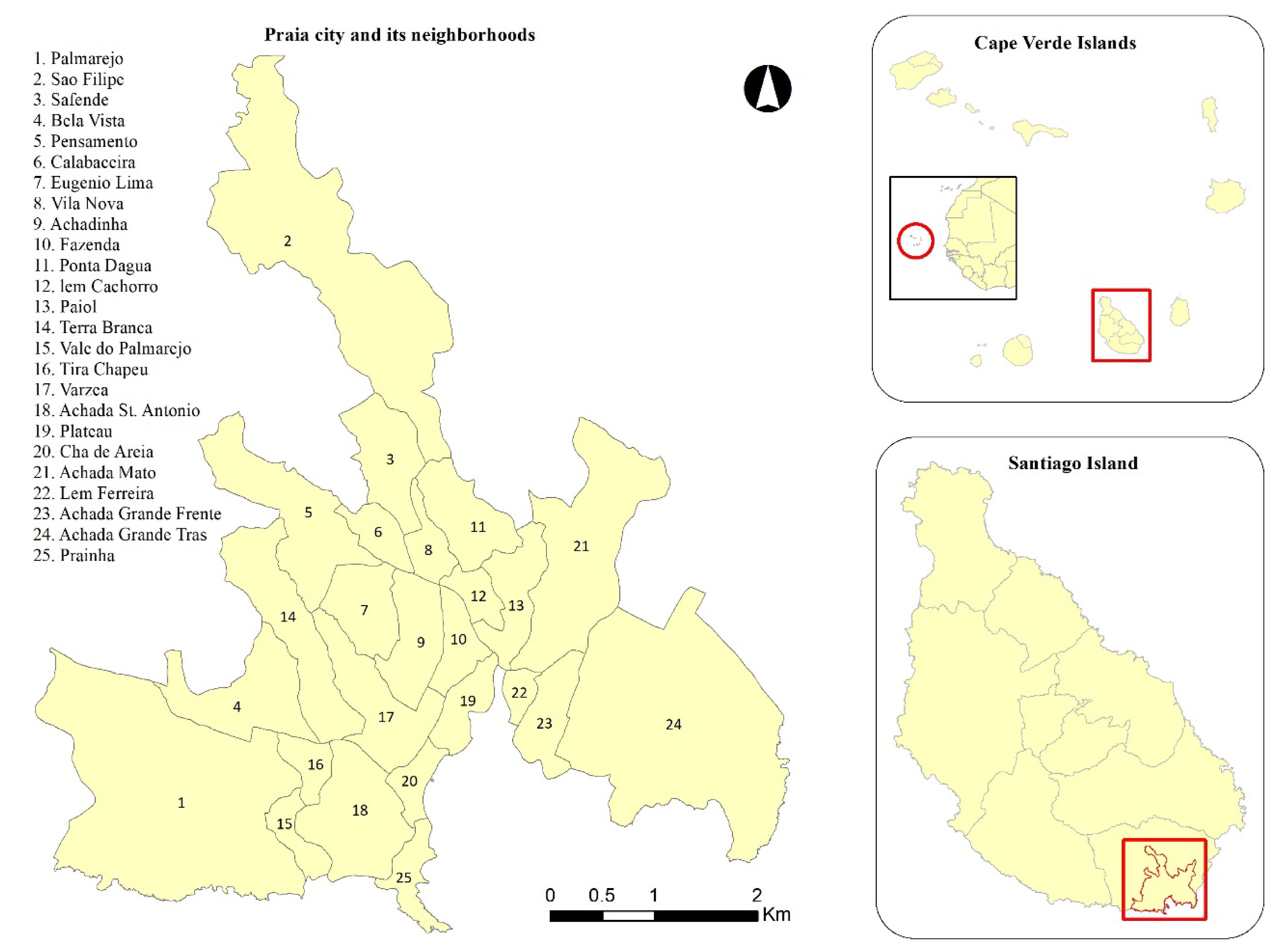
The 10 islands of Cape Verde are located on the West African coast, 450 km from Senegal (Figure 1). The island of Santiago has only 24.5% of the national territory and is home to 56% of the country’s entire population, having nine of the 24 Cape Verdean cities, including the capital city of Praia. Praia is the main economic and political center of Cape Verde, located on the southeasternmost end of Santiago Island. Praia city, the capital of Cape Verde, like most of the African cities, has been experiencing an urbanization process quite different from those in developed countries [36], mainly due to an intense movement of people from rural areas to the cities. This intense urbanization, mainly caused by successive years of drought, land degradation, and the emergence of industrial clusters in the cities that offer better opportunities for employment and education [37], has been generating a built environment predominantly dominated by informality and spontaneous land occupation. This intense demographic pressure and mono-polarization of the capital city is also typical in small island developing states (SIDSs). As predicted by Angel [38], until 2030, developing countries, particularly in Africa and Asia, may experience a duplication of their urban population and a triplication of built-up areas. This fast increase of population and built-up areas has engendered many social problems, including crime. In addition, little is known about the relationship between the urban built environment and crime in the African context, which makes the reported conclusions from previous studies limited and regionalized.
In Cape Verde, the city of Praia is the most problematic in terms of land use planning [39]. In 2010, it had 26% of the Cape Verdean population, 42% of Cape Verde’s urban population, and 76.7% of Santiago Island’s population—all this in only 0.25% of the national territory [40]. Moreover, only 20% of the buildings have received formal planning approval, and half of the housing has only one floor. This city is dominated by informal and spontaneous construction [41].
The Praia municipality has 39% and 74% of Cape Verde and Santiago Island’s Gross Domestic Product (GDP), respectively [42]. Thanks to internal migration and the migration of youth and adults from other African countries seeking for employment opportunities generated as a result of foreign and domestic investment, the population of Praia has increased rapidly over the last few decades (3% annually), starting from 38,564 in 1980 to 94,048 in 2000, and about 145,290 in 2015 [40,43]. In parallel, the capital city has registered higher crime rates among Cape Verdeans cities, with a total of 8616 crimes in the year 2017, of which 59% were crimes against property and 41% were crimes against people [44].
The extent of the study area is 33.2 km2 and includes 42 neighborhoods, mostly residential. The neighborhoods’ extent varies from 0.10 km2 and 1.9 km2, with a mean of 0.47 km2. However, in this study, we only considered 25 neighborhoods because we aggregated the neighborhoods in order to match with crime data.

3.2. Materials and Methods

3.2.1. Criminal Data

Criminal events are recorded by the Polícia Nacional de Cabo Verde [44]. In this study, we used criminal statistics from the years 2013–2017 that include a variety of crimes, grouped into two broad categories—crimes against property and crimes against people, which are further sub-classified into smaller groups. The types of crimes used in this study and their subtypes are described in Table A1. Five main types of crimes were selected: burglary, robbery, mugging, residential robbery, and crimes involving weapons. Given that criminal data are count events from neighborhoods with different sizes, proper scaling was carried out in order to make them comparable. Therefore, each type of crime was divided by the hectare of the built-up area (BUA) of its respective neighborhood, taken from Silva and Li [43]. Such output was labelled as crime rates or crime intensity.

3.2.2. Cartographic Data

Cartographic data related to building footprints and roads at scale 1:1000 and one-meter equidistance contour and mass point elevation were obtained from the Instituto Nacional de Gestão de Território of Cape Verde [45,46].

3.2.3. Socioeconomic Data

From the Instituto Nacional de Estatística de Cabo Verde [47], we obtained unemployment rates and socioeconomic and income data at the neighborhood level. Socioeconomic data were used to develop a household socioeconomic variable [43]—the percentage of the household family with possession and use of certain goods and services; and income data was used to create a per cent low-income household family—monthly income less or equal to 15,000 CVE (about $149 USD).

3.2.4. The UBEIs Selection and Calculation

To measure the quality of the urban built environment of each neighborhood in relation to crimes opportunities, four intrinsic and two extrinsic indicators were calculated. In this section, we presented and described the six different UBEIs applied in this study. Additionally, intrinsic non-correlated UBEIs were linearly combined to represent a single urban built environment indicator (CUBEI).
The neighborhoods’ intrinsic UBEIs were developed based on buildings footprints: road nodes density (RND), road surface density (RSD), percentage of open spaces (POS) and roads layer—regular street nodes (RegSI), road network complexity (RNC), and ETA index. Furthermore, two complementary extrinsic indicators were developed: neighborhood ages (NAge) and percentage of free shared boundaries (PFSB).

Road Nodes Density (RND) and Road Surface Density (RSD)

The RND is the number of street nodes per hectare of urban patches and the RSD is the ratio between the total area occupied by roads and the total amount of urban patches in each particular neighborhood.

Regular Street Index (RegSI)

RegSI basically quantifies the degree of planning of the urban environment of each particular neighborhood. This variable can be expressed as the ratio between numbers of orthogonal or regular intersections nodes and the total number of roads intersections nodes in each particular neighborhood. Third and fourth-degree order of roads intersections were considered. Fourth-degree order nodes are those nodes where four roads meet (Figure 2a,c), and third-degree order nodes are those where three roads meet (Figure 2b,d).
A GIS technique was performed to count the number of orthogonal intersections. A two-meter buffer ring at roads intersections was generated and then split by their corresponding intersected roads edges, generating a set of sectors polygons of each buffer unit. In addition, the proportion of the area of each sector in relation to the area of buffer was calculated. Based on this area proportion, different orders of orthogonal roads intersections were selected and then counted within each neighborhood using the spatial join technique. A threshold value of 23% to 27% in the per cent area of each sector was applied in the nodes selection process.

Road Network Complexity (RNC)

From a topologically corrected street network, split at nodes intersections, the street orientation was calculated using the python script (see Appendix B, Code (B.1)) and then intersected with neighborhood shapefile in order to have linked each road segment to its respective neighborhood. We have considered 24 bin of azimuth angle of 15 degrees each in order to capture more heterogeneity of streets orientation within and between neighborhoods.
WBSP ix = PSE i   ·   PSL i 2 ,
where WBSPix is the weighted average street proportion in bin i in neighborhood x; PSEi and PRLi is the percentage of street edges in the bin i and percentage of street length in bin i, respectively.
RNC = n = 1 n ( MAX ( WBSP ix ) ) WBSP ix ,
where RNC is the neighborhood road network complexity index, WBSPix is the weighted average street proportion in bin 1 to n in neighborhood x.
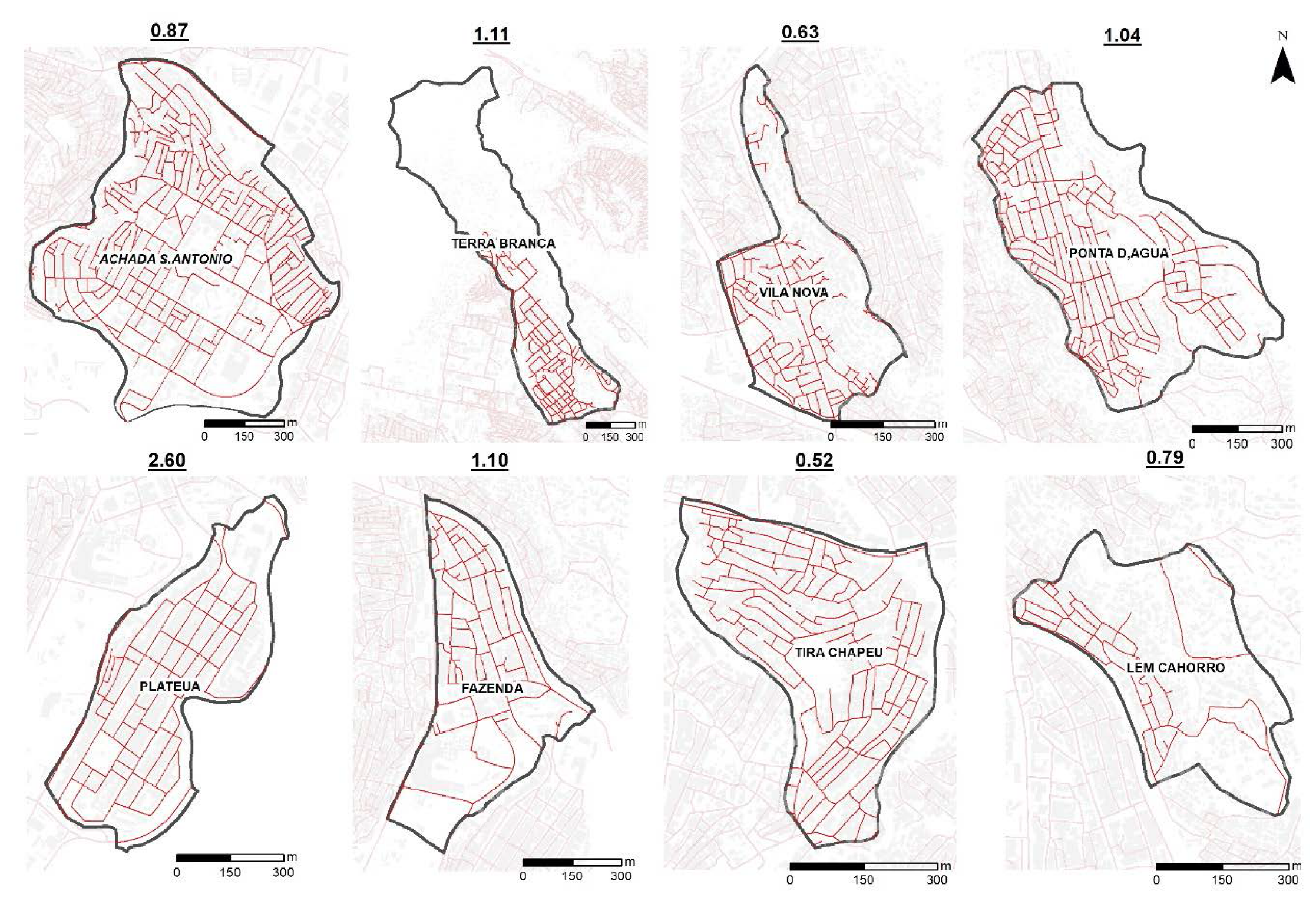
The difference between the bin with higher proportions and all the others bin in each particular neighborhood shown in Equation (2) allows us to capture the heterogeneity of the street networks within each neighborhood (Figure 3). For instance, for a neighborhood whose streets are more or less regular, the bin proportions difference will be higher because few bins will have high proportions and many bins will have small proportions, which tend to increase its index (see plateau neighborhood in Figure 3). On the other hand, in the neighborhood where streets are very irregular, the probability to have significant proportions of streets in each bin is higher, or in other words, the proportions between bins tend to be more or less the same, which will result in a smaller difference between bins and lower index (see Eugenio Lima and Calabaceira in Figure 3). However, because some neighborhoods (e.g., Lém Cachorro, Safende) have a significant amount of their built-up areas without roads coverages, this indicator should be adjusted by this factor. Therefore, we performed a selection by location of building footprints farther than 100 m from roads and their corresponding percentage of area in relation to the total built-up area within each respective neighborhood. This proportion was used as a function of RNC index stabilization. For example, Lém Cachorro has an RNC index of 0.79, and 27% of its built-up area is uncovered by roads. Therefore, the RNC index is reduced by 27%, ending up with an adjusted index of 0.58.

Percentage of Open Spaces (POS)

The ratio between the area occupied by buildings and roads (merged), and the area of urban patches in each particular neighborhood—previously delineated by Silva and Li [43]—indirectly define the degree of dispersion of the buildings and roads. This approach is a small adjustment of what Jaeger et al. [48] called the percentage of built-up area (PBA).
POS = 1 A bup A up ·   100 ,
where POS is the percentage of open spaces in the neighborhood x, Abup sum of the built-up areas (roads and buildings) in the neighborhood x, and Aup is the area of the urban patches in the neighborhood x.

ETA Index

Eta index is the ratio between the total street lengths (TSL) and a number of streets edges (NSE) within each particular neighborhood. It basically defines the mean size of street edges.
ETA = i SL i SE ,

Neighborhood Age (NAge)

The NAge was calculated using the proportion of built-up areas in each neighborhood at each corresponding year (1969, 1993, 2003, 2010, and 2015) derived from Silva and Li [43]. First, we subtracted each year (1969, 1993, 2003, 2010 and 2015) from the year 2015, resulting in years differences of 42, 22, 12, 5, and 0. Second, this year’s differences were multiplied by their corresponding area proportion in order to obtain an approximated average age of the neighborhood.
NAge = ( LP Y ) ·   PBUp ,
where NAge is the average neighborhood age, LP is the most recent data indicating year of built-up areas available, Y is the individual time period, and PBUp is the proportion of built-up area in period Y.

Percentage of Free Shared Boundaries (PFSB)

Shared boundaries are the common boundaries between neighborhoods without any kind of natural barrier. Natural barriers are areas with a slope greater than 25% and located at most 100 m from the boundary of the neighborhoods or large open spaces and discontinuity in urban patches (greater than 200 m). Praia is a city with significant variations in its topography with some neighborhoods sited on plateaus and others in valleys and this effect must be taken into account because it influences the relationship between them. The boundaries of the neighborhoods are mostly defined on those higher slope areas. The slope was calculated using a digital elevation model generated from a one-meter equidistance contour [46]. Regions with a slope greater than 25% were extracted and converted to a polygon shapefile. In order to select the border that intersects the steepest slope areas, the boundaries line features were split at vertices using GIS tools, which breaks the boundaries into smaller lines. This procedure allows us to select by location those lines within a 100-m distance from the natural barrier and to obtain the natural barriers on the shared boundaries of each the neighborhood. The PFSB was calculated by the ratio of free shared boundaries and the perimeter of the neighborhood, indicating the degree of external influence in each neighborhood. The higher the PFSB, the more interaction with surrounding neighborhoods.

3.2.5. The UBEIs Standardization

Having computed the UBEIs for each of Praia neighborhood, these variables was scaled in a range between 0 (favorable for crimes) and 1 (unfavorable for crimes), using the following formula:
X New = X   i X min X max   X min ,
where XNew is the scaled UBEI, Xi is the actual value of UBEI, and Xmin and Xmax are the minimum and maximum value of UBEI, respectively. The value of UBEI, which empirically isinversely related to crimes rate, was inverted in order to have a logical indicator. This min-max standardization approach is simple to apply and is widely used in GIS and machine learning in order to make multiples variables of different units comparable by fitting the data points into a specific predefined range.

3.2.6. Filtering of the UBEIs

Most of the parametric statistics require some assumptions such as the number of observations, the number of variables, linear relationship, and specific variables type, absent of outliers and data normality. In contrast, Spearman’s rank-order correlation statistic approach is nonparametric (distribution-free). It measures the strength of monotone association between two variables and is not a measure of the linear relationship between two variables [49]. Although we have observed some trend of the linear relationship between UBEIs and different crimes rates, the data presented some outliers, which makes Spearman’s correlation coefficient more appropriate than Person’s correlation.
Bivariate correlations among the candidate predictors were calculated (Table 1), in order to avoid redundancy explanatory power in combining the UBEIs. We assumed as danger level of correlation value equal to or greater than 0.7, represented in bold in Table 1. The RND, RSD and NAge are highly correlated (ρ ≥ 0.7; Sig. ≤ 0.01) with POS. Likewise, ETA is correlated with RND (ρ ≥ −0.85; Sig. ≤ 0.01) and therefore, since RND is removed from our analysis, ETA is kept. Non-statistically high correlation was found between the remaining intrinsic UBEIs, suggesting their relevance of representing independent component of the UBE. However, the NAge presented statistically significant high correlation with POS, then, we excluded it from our analysis. Therefore, only PFSB is used as extrinsic indicators of UBE and was not mixed with intrinsic indicators.

3.2.7. Exploring the Link between UBE and Crimes

Bivariate Spearman correlation coefficient was performed between all the individuals’ UBEIs and the five types of crimes analyzed in this study in order to explore their relationship. The linear combination (summation) of the standardized variables—intrinsic indicators (see Section 3.2.4)—was carried out to introduce a new and single indicator of urban built environment (CUBEI) that reflects the quality of the urban environment based on the principles of CPTED. Then, the Spearman correlation was performed in order to understand its relationship with the five different types of crimes (burglary, robbery, mugging, residential robbery and crimes involving weapons). To control for other socioeconomic variables, ordinary least squares (OLS) regression was also performed using crimes intensity as dependent variable and CUBEI, PFSB, socioeconomic indicators, income and unemployment rate as independent variables.

4. Results

4.1. Relationship between UBEIs and Crime Types

Table 2 shows the bivariate Spearman correlation coefficient between different types of crime rates and the UBEIs. Overall, we observed a substantial correlation between the UBEIs and different types of crime rates, with the exception of RegSI which did not correlate with any type of crime. The ETA index and PFSB showed an association with all types of crimes, and both were highly correlated with crimes involving weapons. In addition, the PFSB is also highly correlated (ρ = 0.726, sig. ≤ 0.01) with mugging. An increase in RNC indicator is associated with a consistent decreasing rate in all types of crime, with the exception of burglary crimes, however, stronger for residential robbery (ρ = −0.665; Sig. ≤ 0.01) and crimes involving weapons (ρ = 0.649, Sig. ≤ 0.01). Likewise, the POS has a strong correlation with burglary (ρ = −0.842; Sig. ≤ 0.01) and a moderate association with robbery, crimes involving weapons and muggings. On the other hand, neighborhood age (NAge) is strongly correlated with burglary and it presented a statistically significant correlation with the other types of crimes, except for residential robbery (ResRob).
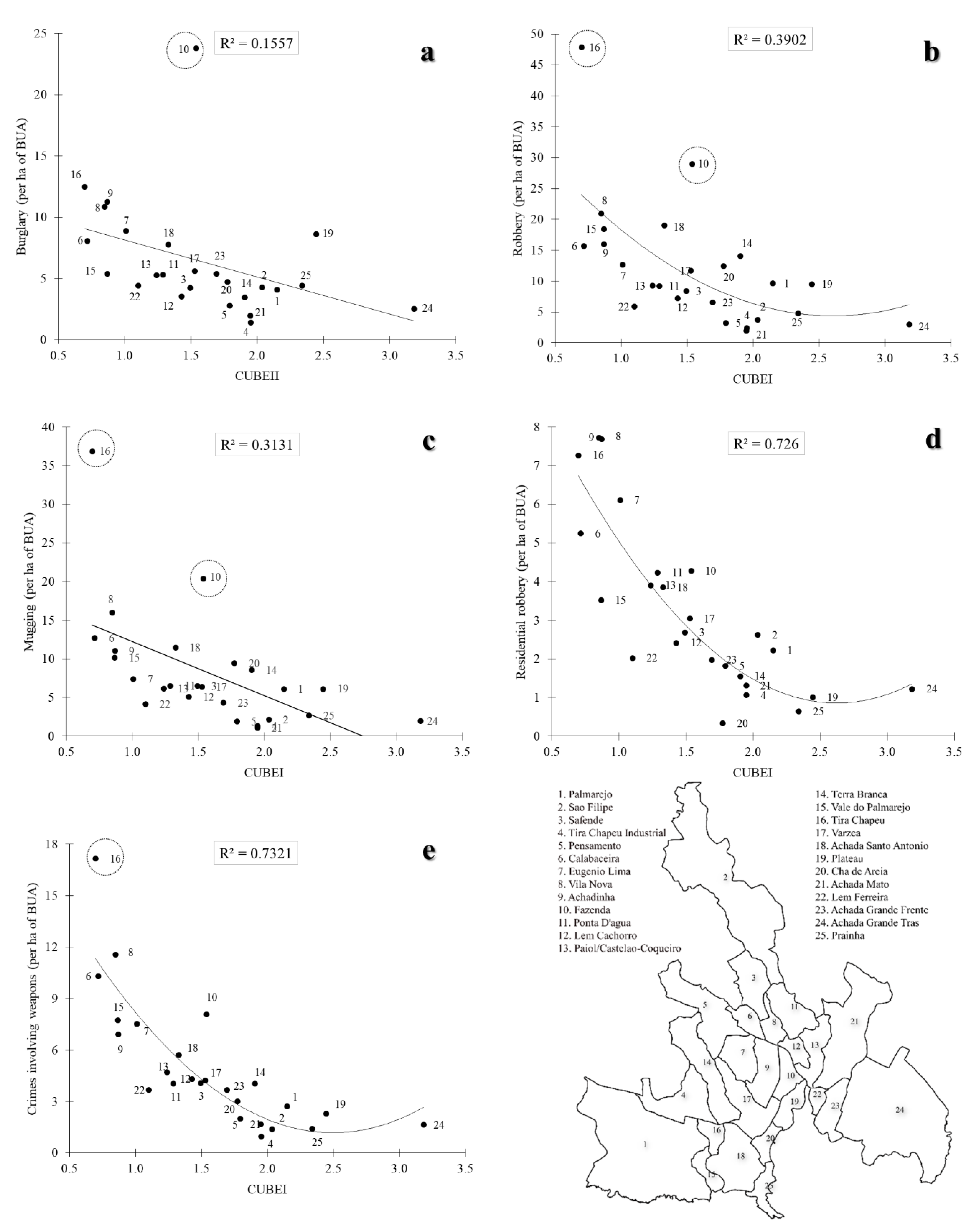
Figure 4 shows the trend of the relationship between the CUBEI and different types of crimes (burglary, robbery, mugging, residential robbery and crimes involving weapons) in the city of Praia. The scatterplot in Figure 4 shows an overall negative relationship between CUBEI and all types of crime. Crimes involving weapons and residential robbery show a much higher degree of correlation comparing with the remaining types of crimes which present a weaker association, although statistically significant. In particular, the neighborhood of Fazenda (id = 10) (Figure 4a–c), where the “sucupira” (local market) is located, presented a dissimilar behavior with the remaining neighborhoods, regarding the burglary, robbery and mugging. Likewise, concerning burglary, Plateau—the historic center of the city where major business and services are sited, also slightly differs from the observed general trend. Figure 5b (robbery), Figure 5c (mugging), and Figure 5e (crimes involving weapons), show Tira Chapeu (id = 16) as an outlier in the presented trend. This zone is well known by locals as one of the most unsafe neighborhoods in the city.
Table 3 shows the Spearman correlation coefficient between the CUBEI and the five types of crimes. All types of crimes have shown a statistically significant relationship with CUBEI. This consistency relationship in both, bivariate and regression level (Table 3, Table 4, Table 5, Table 6, Table 7, Table 8 and Table 9), accounting for households’ income, households’ socioeconomic indicators, and unemployment rates, provides good evidence and confidence in our results.
In order to further explore the relationship between CUBEI and crime rates, controlling for other relevant demographic and social variables, regression analysis was performed. A set of independent variables—CUBEI, household socioeconomic indicators, income, PFSB, and unemployment rate—was used in each crime type–specific regression model. However, only those models with two independent variables that met all the regression assumptions and presented adjusted R-squared higher than 0.5 were selected as the best models since we have a limited sample size. The literature recommends one independent variable for every 10 observations [50,51] in order to avoid model overfitting. Explanatory variables which are not presented in the results outputs were excluded for two reasons, was not statistically significant or violated others OLS assumptions [52]. Socioeconomic indicators and the unemployment rate were kept in the model given that they are well supported in the literature as the main factors influencing crimes, and its relationship with crimes is supported by our empirical evidence of study area. Likewise, the observed relationship between CUBEI, PFSB and crimes rates fulfilled our hypothesis and all the regression assumptions.
The results shown in Table 4 suggest that the household’s socioeconomic conditions and the CUBEI together explain about 50% of the variations in burglary crime intensity (logged variable). Specifically, the sign of the coefficients indicates that an increase in households’ socioeconomic conditions is associated with an increase in the log of burglary, and an increase in CUBEI is associated with a decrease in the log of burglary crime intensity.
Table 5 indicates that the unemployment rate and the CUBEI explain about 60% of the variations in robberies. Particularly, an increase in both the unemployment rate and the CUBEI is associated with a decreasing in robberies. A similar relationship was observed in Table 6, which explains about 55% of the variations in the response variable—mugging.
The PFSB and the CUBEI explain about 68% of the variation in the residential robberies (Table 7). Specifically, an increase in the PFSB is associated with an increase in this type of crime. Likewise, as previously observed in other types of crimes, an increase in CUBEI is associated with a decreasing in residential robberies. Finally, in Table 8 unemployment rate and CUBEI explain about 70% of the variations in crimes involving weapons. When statistically significant, both of them showed a certain consistency in their negative relationship with crimes.
The tested variable (CUBEI) has presented a consistent and statistically significant relationship with all five types of crimes investigated in this study (Table 9). Likewise, the unemployment rate was consistent and statistically significant associated with robbery, mugging, and crimes involving weapons. The household socioeconomic indicator was statistically significant only for burglary crimes and the PFSB was statistically significant only for residential robbery crimes.

4.2. The Relationship between CUBEI and Crimes

The CUBEI captures the physical spatial arrangement of the neighborhoods, based on the measurement of the orthogonality of the street network (RegSI), the navigability of the streets (RNC), the density of the built-up areas (POS), and the partition of the streets (ETA index). The CUBEI expresses a general indication of the quality of the neighborhoods’ physical environment according to the principle of CPTED and BWT, relative to crime opportunities. From the results, we observed in Table 3 that, overall, all the five types of crimes analyzed in this study have shown a general trend of decreasing as the quality of the neighborhoods’ physical environment improves. This observation is supported by the general principles of CPTED as previously described.
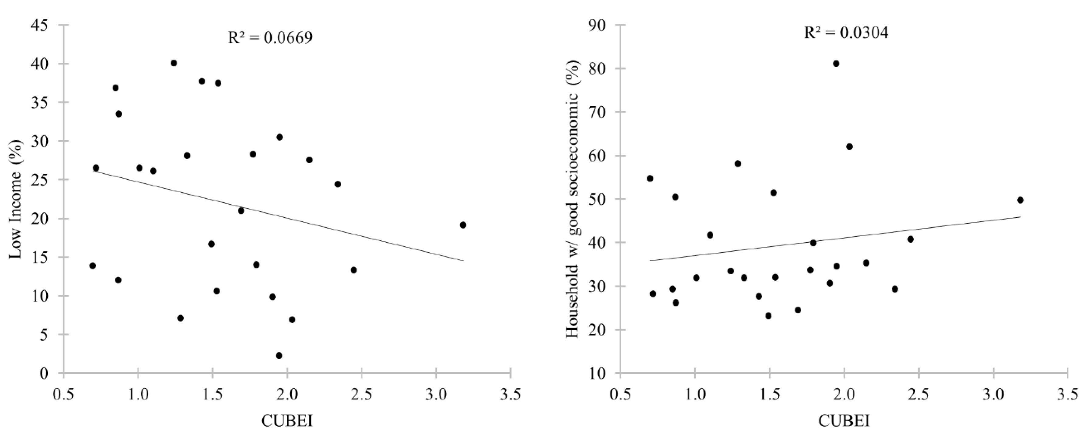
However, since the quality of the urban built environment can be correlated with socioeconomic variables and household’s income, we performed correlation analysis between the CUBEI and socioeconomic variable (ρ = 0.192; Sig. = 0.359) and income (ρ = −0.257; Sig. = 0.215), which were both shown to be not statistically significant. This information (Figure 5) helped us to conclude that the observed relationship between crimes (burglary, robbery, mugging, residential robbery, and crimes involving weapons) and CUBEI is independent to the poverty (i.e., household income, household socioeconomic indicators).

5. Discussion

Given that a very limited number of empirical studies on the relationship between the urban built environment and crimes focus on measuring the physical spatial structure at the neighborhood level by integrating different spatial components and on the moderating effects of socioeconomic factors in developing countries, this study contributes to the literature by providing new and valuable evidence on the relationship between the urban built environment and different specific types of crimes, leading to a deeper understanding of said relationship. In addition, the UBEIs developed in this study (i.e., POS, RNC, and RegSI; NAge and PFSB) will fill the existing gap in the literature and provide better indicators to studies that highly demand UBEIs such as urban planning, energy efficiency, public health/urban walking [34,53], and body mass index [54].

5.1. Effect of UBEIs and CUBEI in Crimes

Overall, the correlation results of the individuals’ UBEIs with different crimes types were statistically significant and consistent with previous studies, with the exception of RegSI, which was not statistically significant. Both extrinsic indicators (NAge and PFSB) were positively associated with all type of crimes studied.
An increase in RNC is associated with a consistent decreasing rate of all types of crimes in the study area. However, it was slightly higher in residential robbery and crimes involving weapons scenario. Legibility is strictly related to the principle of surveillance of CPTED, which states that neighborhoods with complex street networks tend to register more crimes because they are difficult to navigate by both pedestrians and security officers [22,30]. Conversely, according to rational choice theory [5], this is a suitable environment from the offenders’ perspective.
Unlike cities of developed countries, in Praia. the denser neighborhoods are old, informal areas that today are relatively close to the city center. These neighborhoods are denser than those planned neighborhoods or those located in the city center. This fact justifies our findings that as POS increases, the crime rates decrease, meaning that very compact urban environments lead to higher crime rates, especially burglary, because compact neighborhoods tend to diminish the visibility between houses and increase social friction [7,22]. In opposition, open spaces improve visibility, reduce the fear of crimes, and promote safety. Another fact is that in Praia, very dense neighborhoods generally present deficiency in car parking, leading residents to park their cars on street sidewalks, worsening passive surveillance and offering hiding places for criminals.
As hypothesized, neighborhoods where the average street lengths are larger tend to promote better walkability and wider visibility or passive surveillance. This fact may support the negative relationship found between ETA index and crimes rates.
Regarding the extrinsic indicators, neighborhoods with higher PFSB are associated with an increase in crime rates, especially crimes involving weapons (ρ = 0.844), mugging (ρ = 0.726), and residential robbery (ρ = 0.721). In general, these types of crimes are highly dependent on neighbors’ interactions. For instance, empirical evidence has shown that, in Praia, gangs act more in neighboring neighborhoods than in their own for many reasons; they can be easily recognized by the local population, they have a sense of territoriality and ownership, and they have stronger social interaction with locals. Similarly, offenders committing mugging and residential robbery adopt the same strategy. This fact may generate more social friction between neighborhoods leading to higher crime rates [7], particularly the types of crimes mentioned above. In fact, some studies [55] have suggested traffic barriers and road closures as effective crime prevention techniques.
Crimes involving weapons are strongly correlated with CUBEI, which means that the integration of the principles of CPTED and BWT in the urban planning process may result in an overall decrease of this type of crime. In summary, all types of crimes analyzed in this study have shown some degree of association with individuals UBEIs and the CUBEI, which also show some consistency with our expected hypotheses and some previous studies. For example, the relationship between CUBEI and all types of crimes analyzed in this study is supported by the principles of CPTED and the BWT.
From our results (Table 4), socioeconomic indicators presented a positive relationship and CUBEI a negative relationship with burglary, respectively. This indicates that neighborhoods with high socioeconomic indicators are associated with higher burglary rates. This fact may be because high socioeconomic indicators suggest, on the one hand, high neighborhood accessibility and permeability and, on the other, from the offenders’ perspective, higher probability of succeeding in their activities. In contrast, an improvement in neighborhood planning, represented as CUBEI, is associated with a decrease in burglary rate. In fact, BWT posits that neighborhood physical disorder is a key factor for the reproduction of criminals’ activities. In addition, planned neighborhood has both, better passive and active surveillance compared with non-planned neighborhoods. For example, in Praia, police stations are mostly located in planned neighborhoods, and these neighborhoods also present a mixed land-use (residential, commercial, and services) that, according to principles of CPTED, enforce passive surveillance.
The observed effect of the unemployment rate on both types of crime, robbery and mugging (Table 5 and Table 6), contrast with what is hypothesized in previous studies. We observed that an increase in unemployment rate is associated with a decrease in robbery and residential robbery. This effect was expected in our study area, given the reduced size of the neighborhoods. This fact strengthens social relations and territoriality and hence decreases the probability of criminals’ success. Moreover, both types of crimes require physical strength and direct contact with the victims, which is much easier toward strangers.
The observed positive relationship between PFSB and residential burglary suggests that neighborhoods with more connections with closer neighborhoods facilitate the entrance of strangers, which may result in more residential robberies since in theory criminals have their own search radius. On the other hand, this shows that external influence might exist even in cases where Moran I index shows evidence of no spatial dependence. Therefore, there is a need to develop indicators that count for spatial relationship in areas where the irregularity of surface topography masks existing spatial relationship and boundary adjacency.
As previously explained, the contrasting effect of the unemployment rate in robbery and mugging is yet observed in crimes involving weapons. We were expecting to have more crimes involving weapons in neighborhoods with higher unemployment rates, especially because a significant number of this type of crime has its origin from gangs called “thugs” in the Praia suburbs. However, as reported by the US Department of State [56] in Praia many street crimes are not reported to the authorities and therefore are not included in official statistics, especially muggings where locals see low probability in recovering their stolen belongings. This fact might be verified more often in the suburbs than in other areas.
Lima [57] refers to Praia as a “broken city, where poverty is engraved in the urban morphology”; however, our results showed a non-statistically significant relationship between poverty (measured by average income and socioeconomic indicators) and the neighborhoods’ UBE characteristics. The results demonstrate some of the advantages of the proposed indicators and argue in favor of their use in the urban built environment studies and many other interrelated fields.

5.2. Methodological Discussion

As previously mentioned, one of the regression analysis assumptions is the independence of the observations; however, geographic data generally presents spatial dependency, which is states in Tobler’s law, that “everything is related to everything else, but near things are more related than distant things.” Since preliminary exploratory data analysis pointed out an absence of spatial autocorrelation of crime intensities, which is reasonable in our study area, where the irregular surface topography weakens the spatial contiguity and connectivity among neighborhoods, ordinary least squares regression was chosen instead of spatial regression.
This study provides a new methodological approach to normalize crime data by using the neighborhood’s built-up area as a variable in the denominator, which is more realistic than population or neighborhood area itself. However, using built-up areas in the denominator assumes that all the crimes happened within its geographical extent, which may not be true in many circumstances for certain types of crime. Despite this limitation, this technique avoids the overestimation of crime intensity in the neighborhood with large administrative boundary but small built-up area. We extended the concept of the urban built environment by introducing new and more complete and realist measurements which are able to capture the spatial arrangement of building footprints and roads providing a sense of the degree of planning (i.e., intrinsic-POS, RegSI, RNC, ETA and extrinsic-Nage, PFSB); filling the existing knowledge gap on the literature, since the physical form of the neighborhood was underestimated and simplified.
Although we developed the CUBEI and we found its effect on different types of crimes, particularly in the city of Praia, Cape Verde, this trend may not be necessarily observed in other geographical regions, especially in developed countries, where there are different urban development processes, socio-economic lifestyles, and social relations. Therefore, we strongly recommend similar studies to be conducted by using a larger number of observations that might produce more accurate and reliable results by including several individual UBEIs as independent variables. The limited number of observations limit the number of independent variables which might be incorporated in the model, leading to model overestimation parameters [50,51]. Moreover, this study is easy to replicate since we have provided sufficient methodological details to calculate both UBEIs and CUBEI. Individual UBEIs are more useful for larger sample size studies, while CUBEI is more valuable in studies conducted in a small study area with a reduced sample size.

5.3. Implications for Healthy City Planning

This study provides an important clue to urban planners and policy-makers to incorporate CPTED principles and BWT in the conceptualization of their urban plans, both in policy and practical terms, in order to reduce the fear and the incidence of crime and to promote safety in the neighborhoods, by designing and arranging the elements of the urban tissue (e.g., roads and buildings, public spaces, etc.) that leads to a healthier urban built environment which promote well-being and quality of life. Specifically incorporating this paradigm encourages walkability, improves air circulation, and promotes mental and sexual health, which positively influence people’s behaviors and attitudes [58,59].
Furthermore, effective holistic urban planning that provides a physical environment for efficient passive surveillance, grid street network design, high legibility, open spaces, regulated routine maintenance and management of urban spaces, and discouragement of under-used streets either in the early design stage or in the modification of the existing urban environment may prevent or minimize the consequences of many others social issues, such as crime and deficient public health. Public health is strictly linked with the built environment. Therefore, urban spaces planned to encourage walkability are beneficial, especially for those more vulnerable to a sedentary life (e.g., the elderly, children, young parents, the unemployed, and the immobile), providing them opportunities to engage in regular daily walking and cycling, thus reducing the risk of diseases and promoting well-being and, consequently, supportive social contact [58].
However, especially in developing countries that are experiencing rapid and intense urbanization processes, effort must be taken so that road network design anticipates the construction of the building in the early planning stage since it establishes the definitive physical structure of the neighborhood that may be crucial for many future interventions. Likewise, urban rehabilitation and interventions should promote land-use diversity, walkability, open spaces and recreational facilities, and safer boundaries between neighborhoods.
6. Conclusions

Based on the vector data of building footprints and street networks, we calculated and developed several UBEIs and applied them to different neighborhoods in Praia. Empirically, these indicators revealed some consistent and meaningful interpretation of the reality of the UBEIs presented at each studied neighborhood.
Although correlation does not imply causation, both Spearman’s correlation coefficient and OLS model showed that the physical form of the urban built environment (urban morphology) is substantially associated with the crime rates. Specifically, poor urban environment (low legibility and degree of planning) is associated with an increase in crime rates, even after controlling for average household income and socioeconomic indicator. There was no statistically significant correlation between the CUBEI and average household income and socioeconomic indicators, suggesting that the CUBEI is an independent variable. The integration of the CPTED principles and BWT may result in more holistic urban plans, and if well implemented, it might save the government considerable financial resources, specifically in the public security sector. Therefore, building implantation and road placement within cities must be planned to promote human health, well-being, and security.

Author Contributions

P.S. and L.L. contributed to the study design and manuscript writing. P.S. designed and performed the analysis. All authors have read and agreed to the published version of the manuscript.

Funding

This study was funded by the National Key R&D Program of China (2017YFB0503701) and the National Natural Science Foundation of China (41871298).

Acknowledgments

We thank Shiliang SU, from School of Resource and Environmental Science, Wuhan University, for his contribution to the design of the manuscript. We cordially thank Constantino Semedo from Camara Municipal da Praia, Euda Miranda from Instituto Nacional de Gestão do Território of Cape Verde for their support in data collection. We also thank Nelson Silva from Polícia Nacional de Cabo Verde for providing us with criminal data. Finally, we extend our gratitude to Ms Kymmala Francis for her contribution in the final editing of the manuscript.

Conflicts of Interest

The authors declare no conflict of interest.

Appendix A. Crimes types used in this study

Table A1. Crimes classification used in this study and their subtypes.
Burglary
(1) Theft on the public realm, (2) residential burglary, (3) theft in the public/private institution, (4) shoplifting, (5) theft on the agriculture property, (6) theft of vehicle.
Robbery
(7) Mugging, (8) mugging using weapons, (9) mugging using white arm, (10) robbery on the public realm, (11) residential robbery, (12) robbery in the public/private institutions, (13) robbery in the shop, (14) robbery in the agriculture properties, (15) robbery of vehicle.
Residential Robbery
(16) Residential robbery
Mugging
(17) Mugging
Muggings using weapons
(18) Muggings involving weapons
Other crimes involving weapons
(19) Corporal offence using a firearm, (20) corporal offence using a white weapon, (21) corporal offence to police personnel using a firearm, (22) corporal offence to police personnel using a white weapon, (23) illegal possession of a firearm, (24) illegal possession of white weapons.
Crimes involving weapons *
* Crimes involving weapons is the sum of other crimes involving weapons and mugging using weapons.

Appendix B. Calculation of streets orientation (azimuth)

Code (B.1). Python code used to calculate the street orientation
180 + math.atan2 ((!Shape.lastpoint.Y! - !Shape.firstpoint.Y!),(!Shape.lastpoint.X! - !Shape.firstpoint.X!)) * (180/math.pi)

References

  1. Hipp, J.R.; Kim, Y.; Kane, K. The Effect of the Physical Environment on Crime Rates: Capturing Housing Age and Housing Type at Varying Spatial Scales. Crime Delinq. 2018. [Google Scholar] [CrossRef]
  2. Sohn, D. Residential crimes and neighbourhood built environment: Assessing the effectiveness of crime prevention through environmental design (CPTED). Cities 2016, 52, 86–93. [Google Scholar] [CrossRef]
  3. Cozens, P.; Love, T. A Review and Current Status of Crime Prevention through Environmental Design (CPTED). J. Plan. Lit. 2015, 30, 393–412. [Google Scholar] [CrossRef]
  4. Davies, T.; Johnson, S.D. Examining the Relationship Between Road Structure and Burglary Risk Via Quantitative Network Analysis. J. Quant. Criminol. 2015, 31, 481–507. [Google Scholar] [CrossRef] [Green Version]
  5. Eck, E.J.; Weisburg, D. Crime Places in Crime Theory. Crime Place Crime Prev. Stud. 1995, 4, 1–33. [Google Scholar]
  6. Gardiner, R.A. Design for Safe Neighborhoods: The Environmental Security Planning and Design Process; National Institute of Law Enforcement and Criminal Justice: Washington, DC, USA, 1978.
  7. Lupton, R. Centre for Analysis of Social Exclusion; London School of Economics: London, UK, 2003; pp. 1–27. [Google Scholar]
  8. Brantingham, P. Crime and Place: Rapidly Evolving Research Methods in the 21st Century. Cityscape 2011, 13, 199–203. [Google Scholar]
  9. Cerda, M.; Morenoff, J.D.; Hansen, B.B.; Hicks, K.J.T.; Duque, L.F.; Restrepo, A.; Diez-roux, A.V. Reducing Violence by Transforming Neighborhoods: A Natural Experiment in Reducing Violence by Transforming Neighborhoods: A Natural Experiment in Medellín, Colombia. Am. J. Epidemiol. 2012, 175, 1045–1053. [Google Scholar] [CrossRef] [Green Version]
  10. Twinam, T. Danger zone: Land use and the geography of neighborhood crime. J. Urban Econ. 2017, 100, 104–119. [Google Scholar] [CrossRef]
  11. Kamalipour, H.; Faizi, M.; Memarian, G. Safe place by design: Urban crime in relation to spatiality and sociality. Curr. Urban Stud. 2014, 2, 152–162. [Google Scholar] [CrossRef] [Green Version]
  12. Pauls, T.; Zywna, D.; Prochilo, K.; White, S.; Christie, F.; Hainer, C. Crime Prevention through Environmental Design Crime Prevention Through Environmental Design: General Guidelines for Designing Safer Communities; City of Virginia Beach’s CPTED committee: Virginia Beach, VA, USA, 2000; p. 34. [Google Scholar]
  13. Wuschke, K.; Song, J.; Spicer, V. Crime in the Built Urban Environment: Exploring the Impact of Road Networks and Land Use on Residential Burglary Patterns. In American Society of Criminology Annual Meeting; PDXScholar: New Orleans, LA, USA, 2016; p. 1. [Google Scholar]
  14. Elgarmadi, A.S.; Özer, Ö. The relationship of crime to the street network using the space syntax theory, Case study Al-khums City-Libya. Int. J. Latest Res. Humanit. Soc. Sci. 2018, 1, 21–27. [Google Scholar]
  15. Liu, J.; Snow, J.; Che, T. Understanding perceived environment quality in affecting tourists’ environmentally responsible behaviours: A broken windows theory perspective. Tour. Manag. Perspect. 2019, 31, 236–244. [Google Scholar] [CrossRef]
  16. Wilson, J.Q.; Kelling, G.L. Broken Windows: The Police and Neighborhood Safety. The Atlantic monthly: Boston, MA, USA, 1982. [Google Scholar]
  17. Chataway, M.L.; Hart, T.C.; Coomber, R.; Bond, C. The geography of crime fear: A pilot study exploring event-based perceptions of risk using mobile technology. Appl. Geogr. 2017, 86, 300–307. [Google Scholar] [CrossRef]
  18. Roof, K.; Oleru, N. Public Health: Seattle and King County’s Push for the Built Environment. J. Environ. Health 2004, 71, 24–27. [Google Scholar]
  19. Deng, W.; Peng, Z.; Tang, Y. A quick assessment method to evaluate sustainability of urban built environment: Case studies of four large-sized Chinese cities. Cities 2019, 89, 57–69. [Google Scholar] [CrossRef]
  20. Umar, F. Understanding Spatial Patterns of Urban Crime in a Developing Country; University College London: London, UK, 2017. [Google Scholar]
  21. Kruger, T.; Landman, K.; Liebermann, S. A manual for Crime Prevention through Planning and Design; CSIR: Pretoria, South Africa, 2001. [Google Scholar]
  22. Amiri, S.; Brooks, K.R.; Vila, B.J.; Daratha, K.B. Natural surveillance characteristics of building openings and relationship to residential burglary. Appl. Geogr. 2019, 102, 99–108. [Google Scholar] [CrossRef]
  23. Jacobs, J. The Death and Life of America’s Cities; Vintage Books: New York, NY, USA, 1961; pp. 1–472. [Google Scholar]
  24. Newman, O. Architectural Design for Crime Prevention; National Institute for Law Enforcement and Criminal Justice: Washington, DC, USA, 1971.
  25. Jeffery, C.R. Crime Prevention through Environmental Design; Hills, B., Ed.; SAGE: Beverly Hills, CA, USA, 1971. [Google Scholar]
  26. Lang, D.L.; Salazar, L.F.; Crosby, R.A.; Donenberg, G.R. Neighborhood Environment, Sexual Risk Behaviors and Acquisition of Sexually Transmitted Infections among Adolescents Diagnosed with Psychological Disorders. Am. J. Community Psychol. 2010, 303–311. [Google Scholar] [CrossRef]
  27. Kim, D.; Park, S. Improving Community Street Lighting Using CPTED: A case study of three communities in Korea. Sustain. Cities Soc. 2017, 28, 233–241. [Google Scholar] [CrossRef]
  28. Loewen, L.J.; Steel, G.D.; Suedfeld, P. Perceived safety from crimes in the urban environment. J. Environ. Psychol. 1993, 13, 323–331. [Google Scholar] [CrossRef]
  29. Sreetheran, M.; Konijnendijk, C.; Bosh, V. Den Urban Forestry & Urban Greening Fear of crime in urban parks—What the residents of Kuala Lumpur have to say? Urban For. Urban Green. 2015, 14, 702–713. [Google Scholar] [CrossRef]
  30. Queensland Government. Crime Prevention through Environmental Design Guidelines for Queensland Part a: Essential Features of Safer Places; Queensland Government: Queensland, Australia, 2007.
  31. Salleh, S.A.; Mansor, N.S.; Yusoff, Z.M.; Nasir, R.A. The Crime Ecology: Ambient Temperature vs. Spatial Setting of Crime The Crime (Burglary). Procedia Soc. Behav. Sci. 2012, 42, 212–222. [Google Scholar] [CrossRef] [Green Version]
  32. Sampson, R.J.; Raudenbush, S.W. Disorder in Urban Neighborhoods—Does It Lead to Crime? Am. J. Soc. 2001, 105, 1–6. [Google Scholar]
  33. Andresen, M.A.; Brantingham, P.J.; Kinney, J.B. (Eds.) Classics in Environmental Criminology; CRC Press; Taylor & Francis: Burnaby, BC, Canada, 2010; ISBN 9780864913098. [Google Scholar]
  34. Martínez, C.F.; Hodgson, F.; Mullen, C.; Timms, P. Walking through deprived neighbourhoods: Meanings and constructions behind the attributes of the built environment. Travel Behav. Soc. 2019, 16, 171–181. [Google Scholar] [CrossRef]
  35. Robinson, A.I.; Carnes, F.; Oreskovic, N.M. Spatial analysis of crime incidence and adolescent physical activity. Prev. Med. 2016, 85, 74–77. [Google Scholar] [CrossRef] [PubMed] [Green Version]
  36. UN-Habitat. Urbanization and Climate Change in Small Island Developing States; UN-Habitat: Nairobi, Kenya, 2015. [Google Scholar]
  37. Lomoro, M.; Babi, A.; Guogping, X.; Leju, J.; Ladu, C. Causes and consequences of rural-urban migration: The case of Juba Metropolitan, Republic of South Sudan. In IOP Conference Series: Earth and Environmental Science; IOP Publishing Ltd.: Zhuhai, China, 2017; Volume 81, p. 012130. [Google Scholar]
  38. Angel, S. The NYU Urban Expansion Program: A Primer; NYU Stern Urbanization Project: New York, NY, USA, 2015; pp. 1–15. [Google Scholar]
  39. Tavares, C. A Política de Solo na Política Urbana: A Sua Relevância na Cidade da Praia—Cabo Verde (The Urban Soil Policy: Its Relevance in the City of Praia—Cape Verde); Universidade Nova de Lisboa: Lisbon, Portugal, 2007. [Google Scholar]
  40. Instituto Nacional de Estatistica de Cabo Verde. Evolução da População Residente Urbana Por Ilha e Concelho, Segundo os Censos de 1990–2010 (Evolution of the Urban Resident Population by Island and County, According to Censuses From 1990–2010); Instituto Nacional de Estatistica de Cabo Verde: Praia, Cape Verde, 2010. [Google Scholar]
  41. Câmara Municipal da Praia. Proposta do Plano Director Municipal (Proposal of the Municipal Master Plan); CMP: Praia, Cape Verde, 2014. [Google Scholar]
  42. Instituto Nacional de Estatistica de Cabo Verde. Produto Interno Bruto (PIB) Por Ilha Série 2007–2012 (Gross Domestic Product (GDP) by Island, Series 2007–2012); Instituto Nacional de Estatistica de Cabo Verde: Praia, Cape Verde, 2015. [Google Scholar]
  43. Silva, P.; Li, L. Mapping Urban Expansion and Exploring its Driving Forces in the City of Praia, Cape Verde, from 1969 to 2015. Sustainability 2017, 9, 1434. [Google Scholar] [CrossRef] [Green Version]
  44. Policia Nacional de Cabo Verde Estatística criminal do comando regional da Praia. 2017; [Excel spreadsheet] (criminal statistics of unpublished raw data).
  45. Instituto Nacional de Gestão do Território Cartografia planimétrica da cidade da Praia. [shapefile] (planimetric data of the city of Praia). 2010; Unpublished raw data. [Google Scholar]
  46. Instituto Nacional de Gestão do Território Dados altimetricos da cidade da Praia. [shapefile] (altimetry data of the city of Praia). 2010; unpublished raw data. [Google Scholar]
  47. Instituto Nacional de Estatistica de Cabo Verde (INE-CV) Condições de vida por zonas—Concelho da Praia. Living Conditions per Zones—Municipality of Praia; INE-CV: Praia, Cape Verde, 2010. [Google Scholar]
  48. Jaeger, J.A.G.; Bertiller, R.; Schwick, C.; Kienast, F. Suitability criteria for measures of urban sprawl. Ecol. Indic. 2010, 10, 397–406. [Google Scholar] [CrossRef]
  49. Hauke, J.; Kossowski, T. Comparison of values of Pearson’s and Spearman’s correlation coefficient on the same sets of data. Quaest. Geogr. 2011, 30, 87–93. [Google Scholar] [CrossRef] [Green Version]
  50. Babyak, M.A. What you see may not be what you get: A brief, nontechnical introduction to overfitting in regression-type models. Psychosom. Med. 2004, 66, 411–421. [Google Scholar] [CrossRef] [Green Version]
  51. Howell, D.C. Statistical Methods for Psychology, 7th ed.; Wadsworth, Cengage Learning: Belmont, NC, USA, 2010; ISBN 9780495597841. [Google Scholar]
  52. Poole, M.A.; Farrell, P.N.O.; Poole, A.; Farrell, N.O. The assumptions of the linear model regression. Trans. Inst. Br. Geogr. 1971, 52, 145–158. [Google Scholar] [CrossRef]
  53. Bornioli, A.; Parkhurst, G.; Morgan, P.L. Affective experiences of built environments and the promotion of urban walking. Transp. Res. Part A Policy Pract. 2019, 123, 200–215. [Google Scholar] [CrossRef]
  54. Sun, B.; Yin, C. Relationship between multi-scale urban built environments and body mass index: A study of China. Appl. Geogr. 2018, 94, 230–240. [Google Scholar] [CrossRef]
  55. Beavon, D.J.K.; Brantingham, P.L.; Brantingham, P.J. The influence of street networks on the patterning of property offenses. Crime Prev. Stud. 1994, 2, 115–148. [Google Scholar]
  56. U.S. Department of State. Cabo Verde 2019 OSAC Crime & Safety Report; U.S. Department of State: Praia, Cape Verde, 2019.
  57. Lima, R.W. Praia urbana: Desigualdade social, pobreza e desafiliação (Urban Praia: Social inequality, poverty and disaffiliation) in Portuguese. In Cabo Verde da Independência a Hoje—Estudos Pós-Coloniais; Luca Bussotti e Severino Ngoenha (Orgs.): Udine, Italy, 2011; pp. 49–66. [Google Scholar]
  58. Barton, H.; Grant, M. Urban planning for healthy cities: A review of the progress of the european healthy cities programme. J. Urban. Health Bull. N. Y. Acad. Med. 2012. [Google Scholar] [CrossRef] [PubMed] [Green Version]
  59. Satcher, D.; Okafor, M.; Dill, J. Impact of the Built Environment on Mental and Sexual Health: Policy Implications and Recommendations. ISRN Public Health 2012, 2012. [Google Scholar] [CrossRef] [Green Version]
Figure 1. Study area location and its neighborhoods.
Sustainability 12 03056 g001
Figure 2. (a) Fourth-degree order roads intersection and orthogonal arrangement, (b) third-degree order roads intersection and orthogonal arrangement, (c) fourth-degree order intersection and non-orthogonal arrangement, and (d) third-degree order intersection and non-orthogonal arrangement.
Sustainability 12 03056 g002
Figure 3. Examples of streets arrangement and their corresponding road network complexity (RNC) index in some neighborhood of Praia city. A higher RNC index in Plateau and lower in Tira Chapéu and Vila Nova.
Sustainability 12 03056 g003
Figure 4. Relationship between different types of crimes (crimes per hectare of built up areas) and the combined urban built environment indicator (CUBEI) in the city of Praia. (a) Burglary and CUBEI, (b) robbery and CUBEI, (c) mugging and CUBEI, (d) residential robbery and CUBEI, and (e) crime involving weapons and CUBEI.
Sustainability 12 03056 g004
Figure 5. Relationship between the percentage of household with low income and CUBEI (left) and percentage of household with good socioeconomic conditions (right).
Sustainability 12 03056 g005
Table 1. Bivariate correlations (ρ of Spearman) between independent variables.
RND *RSD *RegSIRNCPOSETANAgePFSB
Intrinsic UBEIsRND *ρ1
Sig.0.000
RSD *ρ0.458 a1
Sig.0.0210.000
RegSIρ−0.2880.413 a1
Sig.0.1630.0400.000
RNCρ−0.405 a0.2020.613 b1
Sig.0.0450.3340.0010.000
POSρ0.731 b0.799 b−0.1050.0721
Sig.0.0000.0000.6160.7340.000
ETAρ−0.855 b−0.1430.419 a0.583 b0.474 a1
Sig.0.0000.4950.0370.0020.0170.000
Extr. UBEIsNAgeρ0.508 b0.654 b0.066−0.0700.812 b−0.1181
Sig.0.0090.0000.7530.7400.0000.5750.000
PFSBρ0.644 b−0.028−0.436 a−0.618 b−0.302−0.0040.3011
Sig.0.0010.8920.0290.0010.1430.9850.1440.000
a. Correlation is significant at the 0.05 level (two-tailed). b. Correlation is significant at the 0.01 level (2-tailed). * UBEIs removed from further analysis due to high correlation with POS.
Table 2. Bivariate correlation between dependent variables and individuals’ candidate’s independent variables.
RegSI *RNC *POS *ETA *NAge **PFSB **
Burglaryρ0.036−0.352−0.842 b−0.635 b0.715 b0.536 b
Sig0.8640.0850.0000.0010.0000.006
Robberyρ−0.025−0.415 a−0.598 b−0.640 b0.493 a0.693 b
Sig0.9040.0390.0020.0010.0120.000
Muggingρ−0.085−0.438 a−0.621 b−0.682 b0.505 b0.726 b
Sig0.6880.0280.0010.0000.0100.000
ResRob +ρ−0.236−0.665 b−0.142−0.642 b0.0320.721 b
Sig0.2560.0000.4970.0010.8780.000
CrmWp ++ρ−0.369−0.649 b−0.558 b−0.796 b0.444 a0.844 b
Sig0.0690.0000.0040.0000.0260.000
a. Correlation is significant at the 0.05 level (2-tailed); b. Correlation is significant at the 0.01 level (2-tailed). * Intrinsic UBEIs and ** Extrinsic UBEIs. + ResRob—residential robbery, ++ CrmWp—crimes involving weapons.
Table 3. Correlation matrix (Spearman correlation coefficient) between the CUBEI and the five types of crimes.
Crimes Involving WeaponsBurglaryRobberyResidential RobberyMugging
CUBEIρ−0.874 b−0.615 b−0.637 b−0.826 b−0.694 b
Sig.0.0000.0010.0010.0000.000
b. Correlation is significant at the 0.01 level (two-tailed).
Table 4. OLS regression output. Dependent variable = log burglary rate.
VariableCoefficientStd-Errort-StatisticProbabilityVIF
Intercept1.8772100.3047346.1601590.000003 *------------
Household Socioecon0.0241240.0067943.5508650.013798 *1.143540
CUBEI−0.7378460.156932−4.7016980.000611 *1.143540
Number of observations25
Number of Variables3
Adjusted R20.501761
R20.543281
AICc36.227585
F-statistic13.084808Prob(>F), (2, 22) degrees of freedom:0.000180 *
Wald statistic16.814308Prob(>chi-squared), (2) degrees of freedom:0.000223 *
Koenker (BP) statistic4.722746Prob(>chi-squared), (2) degrees of freedom:0.094291
Jarque-Bera statistic0.595898Prob(>chi-squared), (2) degrees of freedom:0.742339
* Statistically significant at 0.05 level.
Table 5. Ordinary least squares (OLS) regression output. Dependent variable = log robbery rate.
VariableCoefficientStd-Errort-StatisticProbabilityVIF
Intercept5.7369620.6691518.5734880.000000 *------------
Unemployment rate−0.1459870.039924−3.6566070.000028 *1.308012
CUBEI−1.1711550.191252−6.1236300.000001 *1.308012
Number of observations25
Number of Variables3
Adjusted R20.600750
R20.634020
AICc42.757055
F-statistic19.056328Prob(>F), (2, 22) degrees of freedom:0.000016 *
Wald statistic52.386302Prob(>chi-squared), (2) degrees of freedom:0.000000 *
Koenker (BP) statistic0.414304Prob(>chi-squared), (2) degrees of freedom:0.812896
Jarque-Bera statistic1.479585Prob(>chi-squared), (2) degrees of freedom:0.477213
* Statistically significant at 0.05 level.
Table 6. OLS regression output. Dependent variable = log mugging rate.
VariableCoefficientStd-Errort-StatisticProbabilityVIF
Intercept5.3443180.7621137.0125050.000000 *------------
Unemployment rate−0.1403830.045471−3.0873350.000903 *1.308012
CUBEI−1.2359700.217821−5.6742390.000008 *1.308012
Number of observations25
Number of Variables3
Adjusted R20.558359
R20.595162
AICc49.261247
F-statistic16.171382Prob(>F), (2, 22) degrees of freedom:0.000048 *
Wald statistic35.206153Prob(>chi-squared), (2) degrees of freedom:0.000000 *
Koenker (BP) statistic0.232570Prob(>chi-squared), (2) degrees of freedom:0.890221
Jarque-Bera statistic2.052713Prob(>chi-squared), (2) degrees of freedom:0.358310
* Statistically significant at 0.05 level.
Table 7. OLS regression output. Dependent variable = square root of residential robbery rate.
VariableCoefficientStd-Errort-StatisticProbabilityVIF
Intercept2.0272440.3836615.2839480.000008 *-----------
PFSB0.0091030.0033882.6865970.005481 *2.259103
CUBEI−0.4391100.173483−2.5311330.017995 *2.259103
Number of observations25
Number of Variables3
Adjusted R20.683028
R20.709442
AICc24.220148
F-statistic26.858253Prob(>F), (2, 22) degrees of freedom:0.000001 *
Wald statistic66.623587Prob(>chi-squared), (2) degrees of freedom:0.000000 *
Koenker (BP) statistic1.022463Prob(>chi-squared), (2) degrees of freedom:0.599757
Jarque-Bera statistic1.618302Prob(>chi-squared), (2) degrees of freedom:0.445236
* Statistically significant at 0.05 level.
Table 8. OLS regression output. Dependent variable = log of crime involving weapons (rate).
VariableCoefficientStd-Errort-StatisticProbabilityVIF
Intercept3.9365570.5301517.4253500.000008 *------------
Unemployment rate−0.0677640.031631−2.1423300.026946 *1.308012
CUBEI−1.1442580.151524−7.5516740.000006 *1.308012
Number of observations25
Number of Variables3
Adjusted R20.707526
R20.731899
AICc31.114637
F-statistic30.029330Prob(>F), (2, 22) degrees of freedom:0.000001 *
Wald statistic34.626691Prob(>chi-squared), (2) degrees of freedom:0.000000 *
Koenker (BP) statistic3.565108Prob(>chi-squared), (2) degrees of freedom:0.168208
Jarque-Bera statistic0.473681Prob(>chi-squared), (2) degrees of freedom:0.789117
* Statistically significant at 0.05 level.
Table 9. Summary of the relationship between independent variables and crime types.
Independent variable (IV)RelationshipType of crime
Household socioeconomic indicator++Burglary
CUBEI+-
Unemployment rate+-Robbery
CUBEI+-
Unemployment rate+-Mugging
CUBEI+-
PFSB++Residential robbery
CUBEI+-
Unemployment rate+-Crimes involving weapons
CUBEI+-
+/- represent the relationships between each IV and the type of crime.