Comparison and Bias-Correction of Satellite-Derived Precipitation Datasets at Local Level in Northern Kenya

Abstract

Understanding ongoing trends at local level is fundamental in research on climate change. However, in the Global South it is hampered by a lack of data. The scarcity of land-based observed data can be overcome through satellite-derived datasets, although performance varies according to the region. The purpose of this study is to compute the normal monthly values of precipitation for the eight main inhabited areas of North Horr Sub-County, in northern Kenya. The official decadal precipitation dataset from the Kenyan Meteorological Department (KMD), the Global Precipitation Climatology Centre (GPCC) monthly dataset and the Climate Hazards Group Infrared Precipitation with Stations (CHIRPS) monthly dataset are compared with the historical observed data by means of the most common statistical indices. The GPCC showed the best fit for the study area. The Quantile Mapping correction is applied to combine the high resolution of the KMD dataset with the high performance of the GPCC set. A new and more reliable bias-corrected monthly precipitation time series for 1983–2014 results for each location. This dataset allows a detailed description of the precipitation distribution through the year, which can be applied in the climate change adaptation and tailored territorial planning.

1. Introduction

Over the past decades, research on climate change has become of primary concern for different disciplines at a global level. However, the understanding of the climate at a local level is key to interpreting undergoing changes. Although there is an abundance of data in the Global North, the countries of the Global South are struggling to fill the gap. More specifically, land-based meteorological stations in African countries are still around half the optimal number required, unevenly distributed and poorly equipped [1,2,3].

In Kenya, there are thirty-two land-based meteorological stations, distributed mainly in the south and on the coast, which are the most developed and geared towards tourism [4]. To improve the livelihoods of communities, enhance and protect property [5], the Kenyan government is promoting the country’s research and development in climate information.

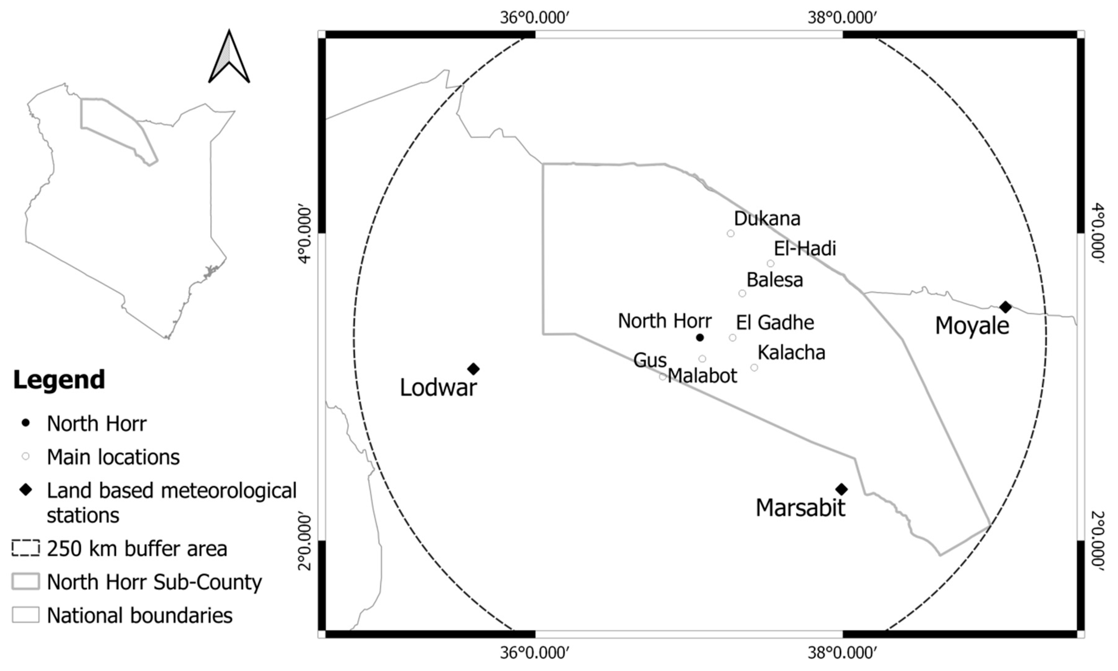
In North Horr Sub-County, situated in Marsabit County in northern Kenya, there are no land-based meteorological stations to provide past climate observations. At a distance of 250 km, there are three weather stations, two located in the highlands and one near lake Turkana. However, they are not close enough to describe the peculiarities of the local climate of North Horr.

The area investigated is mainly inhabited by semi-nomadic pastoral communities which rely on livestock production. They move around the area during the year looking for pasture and water according to the changing season [6]. Climate, therefore, plays an important role in their life, particularly with regard to precipitation, and extreme events such as floods, flash floods and droughts can have a catastrophic impact.

Three complex phenomena and their interaction mainly influence the climate of the Country: the Intertropical Convergence Zone (ITCZ), El Niño Southern Oscillation (ENSO) and the Indian Ocean Dipole (IOD).

Depending on the season, the periodic shift of the ITCZ north and south is mainly responsible for the bimodal rainfall pattern in Kenya. The first rainy season, known as the “long rains season”, lasts approximately from March to May (MAM), and the second, the “short rains season”, from October to December (OND), with some variation across the country. The ENSO and IOD can affect and alter the onset and duration of the rainy and dry seasons triggering events such as droughts and flooding [7,8,9]. In previous decades, changes in the amount of rainfall have been recorded. The northern Arid and Semi-Arid Lands (ASALs) region of Kenya, including Marsabit County, showed a decreasing trend. In particular, the period of 1991–2013 was generally drier than the period 1961–1990 with the MAM season having the highest, yet statistically insignificant, decline in seasonal rainfall amounts [10].

Until recently, climate reference literature for the area consisted of outdated studies [6,11,12]. However, climate change effects on climate at a local scale have increased interest in research studies of the area [13,14,15,16]. This research shows that agro-pastoralists have an awareness of climate change and that the increasing rainfall variability combined with other environmental, social and political pressures negatively affects their resilience [17,18,19,20]. However, although local knowledge is important, if it is not confirmed by official climate information, it could be unusable and ultimately useless [21,22].

The lack of land-based meteorological stations in the area requires the use of satellite-derived data and climatic models for further analysis. The relationship between large-scale weather systems and local climate varies from region to region, making necessary to evaluate and correct them at local scale [23,24], but the scarcity of land surface observation is one of the greatest difficulties in assessing dataset performances [25]. Previous studies have tried to assess the performance of satellite-derived and model-derived datasets in East Africa [26,27,28,29,30,31,32], in particular in Kenya [33,34,35], in order to address the lack of data from land-based meteorological stations. However, these studies have a more regional perspective rather than a local focus, and further investigation on their use at local scale is needed.

This study aims to contribute to precipitation data gap filling in northern Kenya through the design of an innovative methodology for the identification of the normal monthly precipitation values for the main inhabited areas of North Horr Sub-County.

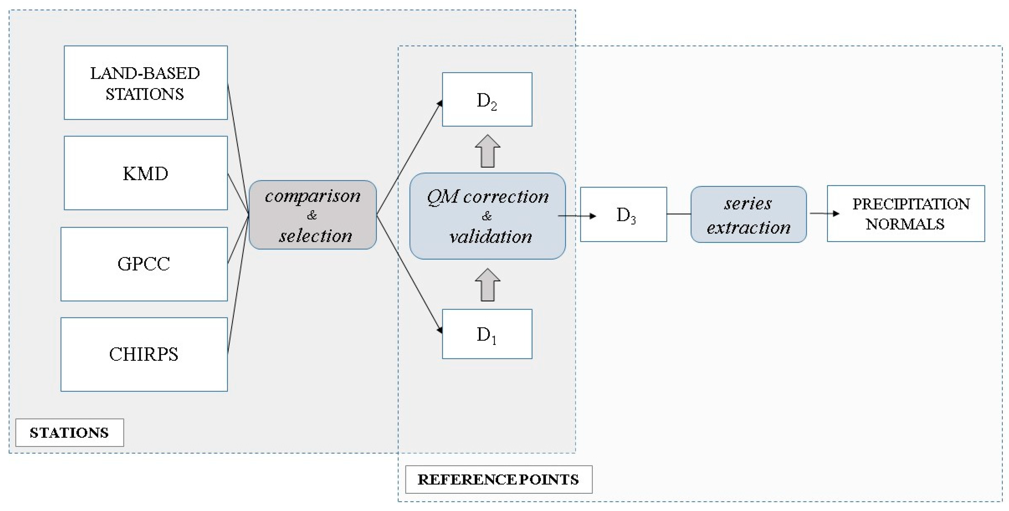
Therefore, it has been necessary to assess and compare the performance of different precipitation datasets with a local scale perspective and to apply a bias correction method, leading to the creation of a new best-fit dataset for the area. Using a direct, point-to-pixel and validation through statistical indices [26,27] approach, this research compares data from models with historical data obtained from land-based meteorological stations in order to assess how well their properties fit the study area characterized by a relatively simple topography. This method was preferred to others due to its adaptability to the available data and to the study area. The no hierarchical k-means clustering method [28] was discarded because of its subjectivity. While it reduces the shortcomings caused by the differences in spatial coverage of the datasets, it requires a subjective choice on the number of clusters of pixels based on the similarity of the annual rainfall cycle. Even an analysis based on the ability of the datasets to detect rainfall events [29] was not suitable because it would have required daily precipitation data instead of monthly data.

Therefore, three model-derived precipitation datasets were selected and compared with the historical series of the nearby land-based meteorological stations of Lodwar, Marsabit and Moyale.

The precipitation datasets used were:

• The decadal dataset from the Kenyan Meteorological Department (KMD), with a resolution of 0.0375°, hereinafter referred to as the KMD dataset [36] available at http://kmddl.meteo.go.ke:8081/SOURCES/.KMD/;
• The Global Precipitation Climatology Centre (GPCC) monthly precipitation dataset, with a 0.5° resolution, hereinafter referred to as the GPCC dataset [37] available at https://www.esrl.noaa.gov/psd/;
• The Climate Hazards group Infrared Precipitation with Stations (CHIRPS) monthly dataset, with a 0.05° resolution, hereinafter referred to as the CHIRPS dataset [38] available at https://iridl.ldeo.columbia.edu/SOURCES/.UCSB/.CHIRPS/.

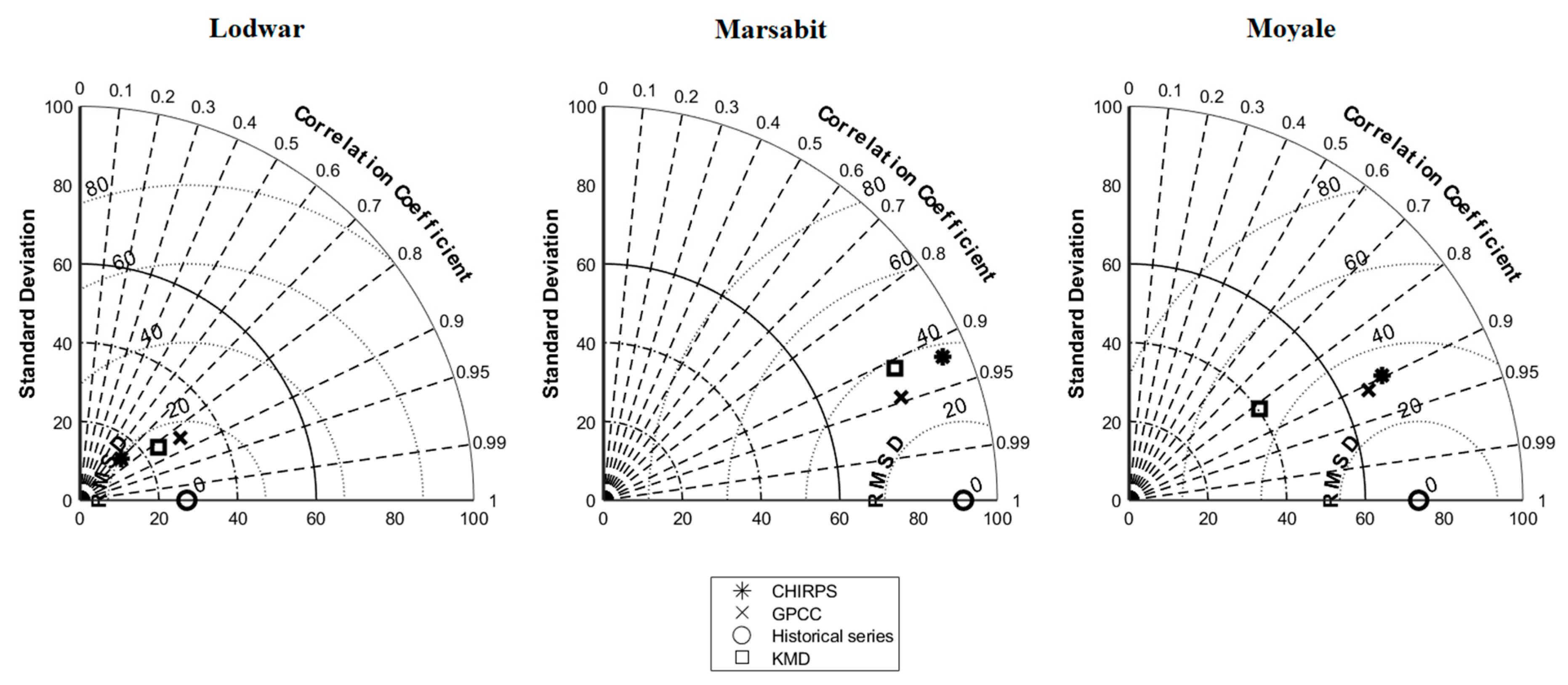
The most commonly used statistical indices were calculated: Bias, Mean Absolute Error, Mean Squared Deviation, Root Mean Squared Deviation, Correlation Coefficient and standard deviation [26,27,28,39,40]. The Taylor diagram was used as a graphical evaluation instrument [41].

The comparative analysis highlighted the relatively high performance of the GPCC dataset and the low performance of the KMD dataset. The GPCC gauge-based dataset selected was used to rectify the KMD dataset at local level on sampled reference points—the main inhabited areas, usually cited in policy planning [42,43]—using the Quantile Mapping [44] bias correction algorithm. Specific normal monthly precipitation values were identified for the reference points.

The new normal monthly precipitation values can be used in future studies for local purposes while the experimented methodology can be applied in other scant data contexts.

In Section 2, the study area is described along with the precipitation datasets that were analyzed. The steps of the methodology adopted are also detailed. In Section 3, the main results are presented. Finally, in Section 4 the conclusions are discussed with particular attention to the limits and to the possible future perspectives of the research.

2. Materials and Methods

2.1. Study Area

The study aims to define the best-fit precipitation dataset for North Horr Sub-County, which is situated in Marsabit County, northern Kenya (Figure 1). The area is considered to be part of the ASALs, with an evaporation rate that exceeds rainfall by more than ten times. However, there are some peculiarities due to the influence of the altitude on the precipitation, which makes Mt. Marsabit (1865 m above sea level), Mt. Kulal (2235 m above sea level), Hurry Hills (1685 m above sea level) and the Moyale-Sololo escarpment (up to 1400 m above sea level) quite wet areas. By contrast, the Chalbi Desert, a large salted depression lying between 435 m and 500 m above sea level, is the dryer feature of the area [45].

There are no land-based meteorological stations in the Sub-County. Therefore, an area within a 250 km radius from North Horr, the main village, has been defined and the meteorological stations located inside this area have been selected. These land-based meteorological stations are situated in Lodwar, Moyale and Marsabit.

The main inhabited areas—i.e., reference points—besides North Horr are Balesa, Dukana, El Gadhe, El-Hadi, Gus, Kalacha and Malabot.

2.2. Precipitation Datasets

Previous studies have assessed the performance of different gridded precipitation products over East Africa [32] and Kenya [34,35]. The comparison of GPCC, CHIRPS, TRMM 3B42 (Tropical Rainfall Measuring Mission) and MERRA Modern-Era Retrospective Analysis for Research and Application) based on eight major agro-ecological zones demonstrated that GPCC and CHIRPS achieved improved results in ASALs [35]. In fact, the GPCC dataset best estimates precipitation in tropical warm semiarid areas while CHIRPS best estimates precipitation in tropical warm arid areas. Similarly, the comparison of CHIRPS, TRMM 3B42, PERSIANN-CDR (Precipitation Estimation from Remotely Sensed Information using Artificial Neural Networks Climate Data Record) and ARC2 (African Rainfall Climatology version 2.0) showed that CHIRPS have excellent performance in ASAL regions (high correlation, low RMSE, and low standard deviation) [34]. At regional level (East Africa), GPCC and CHIRPS have similar consistent results [32]. The other principal gridded precipitation products were evaluated. TRMM 3B42—as well as TRMM 3B43—has a reduced temporal (1998–present) [46] coverage compared to the aim of this research (1983–2013). PERSIANN-CDR underestimates rainfall in different topographical features and climatic conditions [34,47]. MERRA has a coarse resolution (0.5°), best estimates rugged mountainous zones and inaccurately predicts the rainfall amounts in relatively low-lying areas [35]. Following these considerations, three precipitation datasets have been selected and compared (Figure 2). The reference dataset is the KMD dataset provided by the National Meteorological Service. The other two datasets where selected on the base of previous studies results. They are highly reliable because they are provided by the World Meteorological Organization and the Climate Hazard Center funded by the U.S. Agency for International Development (USAID), the National Aeronautics and Space Administration (NASA) and the National Oceanic and Atmospheric Administration (NOAA).

The KMD dataset is a decadal precipitation dataset, part of the Enhancing National Climate Services (ENACTS) project for development in Africa, which focuses on the creation of reliable climate data for national and local decision making. It has been produced by combining quality-controlled data from the national observation network with satellite estimates from the European Meteorological Satellites (METEOSAT). The data processing was performed using the Climate Data Tool software package developed by the International Research Institute (IRI) [36]. The dataset was directly furnished by the KMD but is also available at http://kmddl.meteo.go.ke:8081/SOURCES/.KMD/. It has a spatial resolution of 0.0375° and refers to the period 1983–2014.

The GPCC dataset, a monthly precipitation dataset, was developed by the Global Precipitation Climatology Project in support of the WMO World Climate Research Programme (WCRP) and the Global Energy and Water Cycle Experiment (GEWEX). It is a gauge-only product based on observations from rain gauge stations only available at a coarser resolution of 0.5° and a temporal coverage from 1901 to 2013 [37]. Version 7 (DOI: 10.5676/DWD_GPCC/FD_M_V7_050), available at NOAA/OAR/ESRL PSD website at https://www.esrl.noaa.gov/psd/, has been used for this study.

The CHIRPS dataset was developed to support the USAID Famine Early Warning Systems Network (FEWS NET). It builds on an high resolution and long recording period of precipitation estimates based on infrared Cold Cloud Duration (CCD) observations and on a station blending procedure based on a modified inverse distance weighting algorithm [48]. Several studies ascertain the effectiveness of this dataset in East Africa [26,27,38]. The monthly v2p0 version has been used, which is accessible through the IRI Data Library at https://iridl.ldeo.columbia.edu/SOURCES/.UCSB/.CHIRPS/. It has a spatial resolution of 0.05° and ranges from 1981 to near-present.

Finally, the monthly observed historical series from 1960 to 2016 from Marsabit, Moyale and Lodwar meteorological stations have been used as benchmark for the comparison analysis. They have been directly furnished by the KMD. Their characteristics are summarized in

Table 1. Schematic summary of the meteorological stations’ characteristics.

Station ID	Station	District	Lat	Long	Elevation
63612	Lodwar	Turkana	3.1°	35.6°	523 m
63641	Marsabit	Marsabit	2.3°	37.9°	1345 m
63619	Moyale	Moyale	3.53°	39.1°	1097 m

.

2.3. Methodology

The methodology followed in this study was structured in three steps (Figure 3):

• Section 2.3.1 presents the comparison of the datasets with the observed historical series from the selected land-based meteorological stations. This step lead to the identification and selection of the “reference dataset” (D₁) and “dataset to correct” (D₂).
• In Section 2.3.2, the correction method is detailed. The series from D₂ for each reference point are corrected with D₁ through the Quantile Mapping bias correction algorithm. This procedure leads to the definition of a group of five series for each reference point, each series resulting from a different correction method. The comparison of the five series with D₁ identifies the most appropriate correction method. Consequently, one series for each station and reference point has been selected.
• Section 2.3.3 refers to the extraction and computation of the precipitation normals for each reference point.

2.3.1. Comparison of Dataset Performance at Meteorological Station Level

The performance of KMD, GPCC and CHIRPS datasets have been evaluated by means of a pixel to station comparison with the historical series of the meteorological stations at Marsabit, Lodwar and Moyale over a selected common period from 1983 to 2013. Five statistical indices have been computed: the bias, the Mean Absolute Error (MAE), the Mean Squared Deviation (MSD), the Root Mean Squared Deviation (RMSD) and the Correlation Coefficient (CC) [49]. A comparison of standard deviations (σ) was also performed in order to assess the dispersion of the values with regard to historical values.

A Taylor Diagram has also been created to provide an easier visual interpretation of the results. In the same graph, the CC, the RMSD, and the σ are shown for each series analyzed [41]. The MATLAB SkillMetrics toolbox developed by Peter Rochford has been used to create the diagram [50].

2.3.2. Correction through the Quantile Mapping Method

The KMD dataset, besides being provided by the official National Meteorological Service, has the higher resolution and therefore it was chosen as the dataset to be corrected (D₂).

The GPCC dataset was preferred to the three land-based meteorological stations as reference dataset (D₁). The stations in a 250 km radius, in fact, are not representative of the ASALs, while the GPCC dataset offers reliable interpolated gauge-derived information. This approach, justified by the scarcity of observed data in the region, is in line with previous studies, which aimed to overcome this obstacle by resorting to gauge-derived datasets for the validation of satellite or reanalysis precipitation datasets [51,52]. The correction procedure aims at merging the information derived by the two datasets, namely integrating the satellite-derived data, which is found to have too low level performances, with the gauge-derived data [53,54]. Findings demonstrate that Quantile Mapping can cause inflation problems (same temporal structure and variability of the coarser grid) when applied to datasets of different resolution [55,56]. However, the procedure here used is opposite to the common downscaling procedure; in fact, it aims at correcting a high-resolution satellite-derived dataset with a coarser grid reference dataset.

The KMD dataset was therefore corrected using the Quantile Mapping bias correction algorithm technique, which has been widely used for correction of precipitation datasets [57,58,59] and has demonstrated high performances in arid and semi-arid areas [33,60]. In particular, the work of Ringard et al. demonstrated its usefulness for satellite-derived datasets correction in scarce observed data contexts [61]. Moreover, the Quantile Mapping correction method performs very well concerning the reproduction of the precipitation annual cycle and of the wet and dry periods length [62]. This characteristic is fundamental with reference to the monthly normal identification and for future climate analysis of the area.

The Quantile Mapping technique is based on statistical transformation which attempts to adjust the distribution of modelled data such that it closely resembles the observed climatology solved using a theoretical distribution The ‘qmap’ package developed by Lukas Gudmundsson for R software was used for the computation [63]. The procedure was carried out for all the reference locations using a pixel to pixel approach. The ‘qmap’ package supports five different analytical methods, both parametric and non-parametric transformations. These methods use different functions to transform the distribution of the modelled data to match the distribution of the observations. The five functions performed are parametric transformations (PTF), distribution derived transformations (DIST), non-parametric quantile mapping using empirical quantiles (QUANT), non-parametric quantile mapping using robust empirical quantiles (RQUANT) and quantile mapping using a smoothing spline (SSPLIN)(for further details see the documentation at the following link https://www.rdocumentation.org/packages/CSTools/versions/2.0.0/topics/CST_QuantileMapping).

Five precipitation series were created for the three stations and for the eight reference locations.

The results of the Quantile Mapping correction were compared with the GPCC series for each reference location through the statistical indices (Section 2.3.1). The most appropriate method was identified, leading to the selection of a best-fit precipitation series for each reference location.

2.3.3. Reference Values Computation

New reference values were computed on the new precipitation series by averaging the monthly precipitation amount for the entire period (1983–2013).

3. Results and Discussion

3.1. Comparison of Dataset Performance at Meteorological Station Level

The comparison of the precipitation datasets with the observed series led to an important first conclusion. The KMD dataset does not feature the best indices values for all the stations. Results from the first step of the analysis conducted indicated that the GPCC dataset was a better choice as the reference series.

According to the statistical indices (

Table 2. Comparison based on statistical indices (BIAS, MAE, MSD, RMSD and CC) of the precipitation datasets with the observed historical series from the selected land-based meteorological stations (Lodwar, Marsabit and Moyale) for the period 1983–2013. For the CC index, “*” corresponds to a p-value < 0.01, “**” corresponds to a p-value < 0.001 and “***” corresponds to a p-value < 0.0001. Values in bold correspond to the best value of the index for each station.

	Lodwar			Marsabit			Moyale
	KMD	GPCC	CHIRPS	KMD	GPCC	CHIRPS	KMD	GPCC	CHIRPS
BIAS	0.99	2.52	−5.32	−8.21	2.35	13.40	24.7	5.04	2.16
MAE	5.4	5.74	10.72	14.83	12.7	25.32	29.1	14.9	18.45
MSD	237	260	414	1498	933	1528	2797	966	1087
RMSD	15.4	16.1	20.35	38.71	30.5	39.09	52.9	31.1	32.97
CC	0.83 ***	0.85 ***	0.71 ***	0.91 ***	0.95 ***	0.92 ***	0.82 ***	0.91 ***	0.90 ***

and

Table 3. Comparison based on the standard deviation of the precipitation datasets with the observed historical series from the selected land-based meteorological stations (Lodwar, Marsabit and Moyale) for the period 1983–2013.

Standard Deviation
Lodwar				Marsabit				Moyale
STAT.1	KMD	GPCC	CHIRPS	STAT. 1	KMD	GPCC	CHIRPS	STAT. 1	KMD	GPCC	CHIRPS
27.2	24.1	29.9	14.8	91.4	81.2	79.9	93.4	73.5	40.4	67.0	71.6

¹ STAT. = STATION.

) and to the Taylor diagrams (Figure 4), the GPCC dataset fits better for the stations of Marsabit and Moyale, while the KMD dataset fits better for Lodwar. However, for reasons of homogeneity and consistency, the GPCC dataset was also chosen as the reference dataset for Lodwar station since its statistical values are close to the values obtained for the KMD dataset.

3.2. Correction through the Quantile Mapping Method

As showed in the previous section, the GPCC dataset fits better than the other two datasets compared with the historical series. However, the GPCC dataset has a lower resolution (0.5°) compared to the KMD dataset and CHIRPS dataset (0.0375° and 0.05°, respectively), and the differences in local topography may be biased. Therefore, it was necessary to apply a bias correction method to overcome these two problems. The strategy adopted was to correct the KMD dataset (D₂), which is issued by the official National Meteorological Service and has the highest resolution, with the GPCC dataset (D₁) which performs better on ASALs.

The bias correction method is performed using the Quantile Mapping method from the ‘qmap’ R package. Five different bias-corrected series are obtained based on the five different transformations applied: Parametric Transformations (PTF), Distribution Derived Transformations (DIST), Robust Empirical Quantiles (RQUANT), Empirical Quantiles (QUANT), Smoothing Spline (SSPLIN).

From comparison analysis, the Parametric Transformations method, which fits a parametric transformation to the quantile-quantile relation of observed and modelled values, provided the best results (see Appendix A and Appendix B). Hereinafter, the Bias-Corrected KMD dataset will be referred to as the BCKMD dataset (D₃).

3.2.1. Quantile Mapping Validation at Station Level

The performance of the new BCKMD dataset is assessed by means of the statistical indices mentioned previously (see Section 3.1). The indices have been calculated in relation to the historical series of the land-based meteorological stations, then compared with the same indices calculated for the KMD dataset.

As shown in

Table 4. Comparison based on statistical indices (BIAS, MAE, MSD, RMSD, CC and σ) of the KMD and of the Bias-Corrected KMD (BCKMD) datasets with the observed historical series from the selected land-based meteorological stations (Lodwar, Marsabit and Moyale) for the period 1983–2013. For the CC index, “*” corresponds to a p-value < 0.01, “**” corresponds to a p-value < 0.001 and “***” corresponds to a p-value < 0.0001. Values in bold correspond to the best value of the index for each station.

	Lodwar		Marsabit		Moyale
	KMD	BCKMD	KMD	BCKMD	KMD	BCKMD
BIAS	−0.99	2.29	−8.21	−4.28	−24.74	−5.96
MAE	5.41	7.71	14.83	16.78	29.10	26.02
MSD	237.3	295.32	1498.21	1427.56	2796.62	1881.38
RMSD	15.40	17.18	38.71	37.78	52.88	43.38
CC	0.83 ***	0.83 ***	0.91 ***	0.91 ***	0.82 ***	0.82 ***
Standard Deviation
Lodwar			Marsabit			Moyale
STATION	KMD	BCKMD	STATION	KMD	BCKMD	STATION	KMD	BCKMD
27.15	24.09	29.93	91.44	81.21	81.24	73.54	40.40	67.07

, the BCKMD dataset fits the observed historical series better than the KMD dataset, apart from Lodwar station. This may be due to a higher performance of the KMD dataset—before correction—at Lodwar station compared to the GPCC concerning BIAS, MAE, MSD and RMSD. However, the errors obtained are still acceptably low. In fact, the standard deviation values and the relatively low values of the error’s indices, even for Lodwar, justify the selection of the BCKMD dataset for the study area.

3.2.2. Quantile Mapping at Reference Point Level

The Quantile Mapping correction on the base of the GPCC dataset was also applied to the KMD dataset at the reference points. The Parametric Transformations method has been used in accordance with the validation carried out at the stations level. The result was a best-fit precipitation dataset for the eight locations.

3.3. Calculating Normal Values of Precipitation at Station Level

The normal values were calculated on the precipitation series obtained for the three stations, by averaging the monthly precipitation amount for the entire period (1983–2013) (reported in

Table 5. Comparison of normal values of precipitation (in mm) obtained from the historical time series and the new precipitation dataset BCKMD for the three land-based meteorological stations (Lodwar, Marsabit and Moyale). The table reports monthly cumulative amounts, long rains cumulative amount, short rains cumulative amount and total precipitation amount.

	Lodwar		Marsabit		Moyale
	Historical	Bckmd	Historical	Bckmd	Historical	Bckmd
Jan	6.5	10.7	30.2	31.3	17.4	18.4
Feb	4.2	4.4	19.2	20.8	19.4	21.1
Mar	30.0	33.2	50.2	44.5	53.2	36.0
Apr	38.3	50.9	212.4	195.4	164.9	193.0
May	28.3	37.8	75.1	77.4	100.1	75.3
June	10.6	10.6	10.6	6.7	18.0	9.8
July	12.1	12.4	9.0	3.7	10.2	3.8
Aug	14.5	16.2	8.1	5.1	10.1	7.8
Sep	10.2	13.9	5.3	5.5	15.5	12.9
Oct	11.2	13.9	88.4	87.1	106.6	75.9
Nov	20.4	17.5	139.3	127.3	92.9	79.9
Dec	15.1	7.1	57.5	48.9	28.7	31.6
Long rains	96.6	121.9	337.6	317.4	318.3	304.2
Short rains	46.7	38.5	285.3	263.3	228.1	187.4
Total	201.4	228.6	705.2	653.8	637.0	565.5

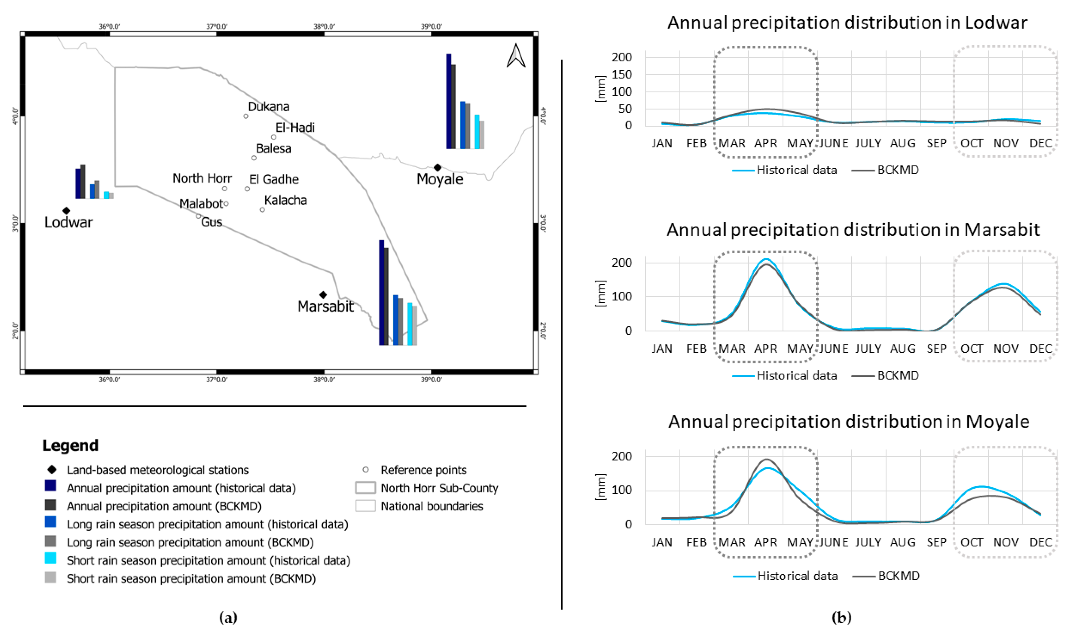
). Long rains amount, short rains amount and total annual amount were also calculated. Figure 5 compares the distribution of the precipitation through the year according to the observed series and to the new BCKMD dataset.

3.4. Calculating Normal Values of Precipitation at Reference Point Level

The normal values were calculated on the precipitation series obtained for each reference point, by averaging the monthly precipitation amount for the entire period (1983–2013). Moreover, long rains amount, short rains amount and total amount were calculated.

The normal values for the eight reference points are shown in

Table 6. Normal values of precipitation (in mm) for the eight reference points in North Horr Sub-County. The table reports monthly cumulative amounts, long rains cumulative amount, short rains cumulative amount and total precipitation amount for each reference point.

	Balesa	Dukana	El Gadhe	El-Hadi	Gus	Kalacha	Malabot	North Horr
Jan	23.3	28.6	19.8	37.0	16.8	19.0	22.1	22.0
Feb	12.3	25.0	10.9	26.4	6.6	13.9	7.6	6.1
Mar	38.3	54.2	35.4	63.1	24.0	30.3	35.0	36.8
Apr	66.8	91.5	55.1	104.2	46.6	57.7	50.3	50.7
May	21.1	29.3	24.4	37.1	19.0	27.5	26.4	26.3
June	6.0	13.8	4.5	11.7	10.9	3.2	7.4	7.0
July	2.7	7.6	1.7	7.2	4.1	1.0	1.9	2.9
Aug	4.5	7.8	5.4	9.8	6.4	3.7	6.0	6.0
Sep	3.5	11.4	2.3	8.3	5.3	1.1	2.4	2.5
Oct	17.7	29.5	14.3	32.7	12.8	16.4	15.4	14.7
Nov	35.9	55.4	21.6	58.8	20.7	19.2	21.7	21.9
Dec	19.3	35.0	13.6	33.9	10.2	14.4	12.6	10.7
Long rains	126.2	175	114.9	204.4	89.6	115.5	111.7	113.8
Short rains	72.9	119.9	49.5	125.4	43.7	50	49.7	47.3
Total	251.4	389.1	209	430.2	183.4	207.4	208.8	207.6

. A visual representation of the precipitation distribution at local scale is pictured in Figure 6.

The understanding of climate differences at local scale is crucial for an effective territorial planning against negative impact of climate change. This study succeeded in obtaining normal values of precipitation for each reference point despite the lack of land-based meteorological stations in the area and high-resolution and fitting satellite-derived precipitation time series. Differences in rainfall regime are evident in Figure 6, which shows higher precipitation amounts in the northern part of the Sub-County then in the southern reference points.

The new precipitation time series can be used for the evaluation of drought indices as well as for water security assessment. More specifically, the monthly normal values can be used as reference values for comparing measured or forecasted data in order to evaluate drought or wet periods.

Moreover, it has been possible to calculate the normal values for the entire long rain season and short rain season, by cumulating monthly values for March, April and May and for October, November and December, respectively. Knowing the distribution of the precipitation throughout the year and the possible deviation from normal values is fundamental. This is at the base of the community organization for the local semi-nomadic pastoral population.

4. Conclusions

The aim of this study was to obtain the normal values of the monthly amount of precipitation for the main inhabited areas in North Horr Sub-County, in order to provide a benchmark for understanding the ongoing changes in the local climate. Therefore, it was necessary to identify an appropriate historical precipitation series. The comparison between the GPCC, KMD and CHIRPS datasets highlighted the lower performance of the KMD dataset compared to the others, despite it being the dataset officially issued and used by the Kenyan Meteorological Department for the whole country. Previous studies on East Africa indicated the CHIRPS dataset to be a reliable global dataset for the region [26,27,32]. The relatively high performance of the GPCC dataset in northern arid Kenya is in line with the results of previous studies, which indicated it as a good fit for the ASALs [35], but with a low capacity in representing complex terrain [28]. However, the need to highlight local differences in the annual trend of precipitation led to the use of the KMD dataset after a correction procedure based on the GPCC dataset. This approach aimed to integrate the higher resolution of the KMD dataset—namely, its ability to detect differences in the precipitation trend at a local scale—with the higher ability of the GPCC dataset to represent the real historical values in the area. The methodology adopted created a new bias-corrected monthly precipitation time series for each reference point, from which the local normal values were extracted.

Since the need for high-resolution precipitation data covering the Global South is becoming urgent for any discipline that must consider the role of climate, this study represents an attempt to provide a solution to the scarcity of observed data. The absence of land-based meteorological stations in the area, however, cannot be ignored and constitutes a limit in the study. Future research should be directed to test the methodology proposed here in other contexts, where the availability of observed data could provide a yardstick for its usefulness and accuracy.

References

1. Hellmuth, M.E.; Moorhead, A.; Thomson, M.C.; Williams, J. (Eds.) Climate Risk Management in Africa: Learning from Practice; International Research Institute for Climate and Society (IRI), Columbia University: New York, NY, USA, 2007. [Google Scholar]
2. Dinku, T.; Block, P.; Sharoff, J.; Hailemariam, K.; Osgood, D.; del Corral, J.; Cousin, R.; Thomson, M.C. Bridging critical gaps in climate services and applications in africa. Earth Perspect. 2014, 1, 15. [Google Scholar]
3. LTS International. Acclimatise Technical Report 8: Availability and Accessibility to Climate Data for Kenya. 2012, pp. 1–47. Available online: https://www.kccap.info/index_option_com_phocadownload_view_category_id_37_Itemid_54.html (accessed on 20 January 2020).
4. Kenya Meteorological Department. Available online: https://www.meteo.go.ke/ (accessed on 5 January 2020).
5. Kenya Meteorological Department. Meteorology Policy 2019; Kenya Meteorological Department: Nairobi, Kenya, 2019. [Google Scholar]
6. MoALF Climate Risk Profile for Marsabit. County Kenya County Climate Risk Profile Series 2017; Government of Kenya: Nairobi, Kenya, 2017.
7. Orindi, V.A.; Ochieng, A. Case Study 5: Kenya Seed Fairs as a Drought Recovery Strategy in Kenya. IDS Bull. 2005, 36, 87–102. [Google Scholar]
8. Karanja, F.; Mutua Nairobi, F. Reducing the impact of environmental emergencies through Early Warning and preparedness-the case of el Niño-Southern Oscillation (ENSO); Nairobi: UNFIP/UNEP/NCAR/WMO/DNDR/UNU. 2000; Available online: https://profiles.uonbi.ac.ke/coludhe/publications/reducing-impacts-environmental-emergencies-through-early-warning-and-preparedne (accessed on 7 January 2020).
9. Ogalo, L.; Owiti, Z.; Mutemi, J. Linkages between the Indian Ocean Dipole and East African Rainfall Anomalies. J. Kenya Meteorol. Soc. 2008, 2, 3–17. [Google Scholar]
10. Ouma, J.O.; Olang, L.O.; Ouma, G.O.; Oludhe, C.; Ogallo, L.; Artan, G. Magnitudes of Climate Variability and Changes over the Arid and Semi-Arid Lands of Kenya between 1961 and 2013 Period. Am. J. Clim. Chang. 2018, 7, 27–39. [Google Scholar]
11. Edwards, K.A.; Field, C.R.; Hogg, I.G.G. A Preliminary Analysis of Climatological Data from the Marsabit District of Northern Kenya; UNEP-MAB Integrated Project in Arid Lands: Nairobi, Kenya, 1979. [Google Scholar]
12. Schwartz, H.; Shaabani, S.; Walther, D. Range Management Handbook of Kenya, Marsabit District; Ministry of Livestock Development, Republic of Kenya: Nairobi, Kenya, 1991.
13. Ongoma, V.; Chen, H.; Omony, G.W. Variability of extreme weather events over the equatorial East Africa, a case study of rainfall in Kenya and Uganda. Theor. Appl. Climatol. 2018, 131, 295–308. [Google Scholar]
14. Schmocker, J.; Liniger, H.P.; Ngeru, J.N.; Brugnara, Y.; Auchmann, R.; Brönnimann, S. Trends in mean and extreme precipitation in the Mount Kenya region from observations and reanalyses. Int. J. Climatol. 2016, 36, 1500–1514. [Google Scholar]
15. Shongwe, M.E.; van Oldenborgh, G.J.; van den Hurk, B.; van Aalst, M. Projected Changes in Mean and Extreme Precipitation in Africa under Global Warming. Part II: East Africa. J. Clim. 2011, 24, 3718–3733. [Google Scholar]
16. Omondi, P.A.; Awange, J.L.; Forootan, E.; Ogallo, L.A.; Barakiza, R.; Girmaw, G.B.; Fesseha, I.; Kululetera, V.; Kilembe, C.; Mbati, M.M.; et al. Changes in temperature and precipitation extremes over the Greater Horn of Africa region from 1961 to 2010. Int. J. Climatol. 2014, 34, 1262–1277. [Google Scholar]
17. Opiyo, F.; Wasonga, O.V.; Nyangito, M.M.; Mureithi, S.M.; Obando, J.; Munang, R. Determinants of perceptions of climate change and adaptation among Turkana pastoralists in northwestern Kenya. Clim. Dev. 2016, 8, 179–189. [Google Scholar]
18. Herrero, M.; Addison, J.; Bedelian, C.; Carabine, E.; Havlík, P.; Henderson, B.; Van De Steeg, J.; Thornton, P.K. Climate change and pastoralism: Impacts, consequences and adaptation. Rev. Sci. Tech. 2016, 35, 417–433. [Google Scholar]
19. Ochieng, J.; Kirimi, L.; Mathenge, M. Effects of climate variability and change on agricultural production: The case of small scale farmers in Kenya. NJAS Wageningen J. Life Sci. 2016, 77, 71–78. [Google Scholar] [CrossRef]
20. Judith, C.; Mbogoh, S.G.; Chris, A.-O.; Patrick, I. Smallholder Farmers’ Perceptions and Responses to Climate Change in Multi-stressor Environments: The Case of Maasai Agro-pastoralists in Kenya’s Rangelands. Am. J. Rural Dev. 2017, 5, 110–116. [Google Scholar]
21. Mbaisi, C.N.; Kipkorir, E.C.; Omondi, P. The Perception of Farmers on Climate Change and Variability Patterns in the Nzoia River Basin, Kenya. Perception 2016, 6. Available online: https://www.semanticscholar.org/paper/The-Perception-of-Farmers-on-Climate-Change-and-in-Mbaisi-Kipkorir/40c0f5ee8576faad730e79b0125087c754c7d0c2 (accessed on 7 January 2020).
22. Deressa, T.T.; Hassan, R.M.; Ringler, C.; Alemu, T.; Yesuf, M. Determinants of farmers’ choice of adaptation methods to climate change in the Nile Basin of Ethiopia. Glob. Environ. Chang. 2009, 19, 248–255. [Google Scholar] [CrossRef] [Green Version]
23. Hewitson, B.C.; Crane, R.G. Consensus between GCM climate change projections with empirical downscaling: Precipitation downscaling over South Africa. Int. J. Climatol. 2006, 26, 1315–1337. [Google Scholar] [CrossRef]
24. Ning, L.; Riddle, E.E.; Bradley, R.S. Projected changes in climate extremes over the northeastern United States. J. Clim. 2015, 28, 3289–3310. [Google Scholar] [CrossRef] [Green Version]
25. Wood, A.W.; Maurer, E.P.; Kumar, A.; Lettenmaier, D.P. Long-range experimental hydrologic forecasting for the eastern United States. J. Geophys. Res. D Atmos. 2002, 107. [Google Scholar] [CrossRef]
26. Gebrechorkos, S.H.; Hülsmann, S.; Bernhofer, C. Evaluation of multiple climate data sources for managing environmental resources in East Africa. Hydrol. Earth Syst. Sci. 2018, 22, 4547–4564. [Google Scholar] [CrossRef] [Green Version]
27. Bayissa, Y.; Tadesse, T.; Demisse, G.; Shiferaw, A. Evaluation of satellite-based rainfall estimates and application to monitor meteorological drought for the Upper Blue Nile Basin, Ethiopia. Remote Sens. 2017, 9, 669. [Google Scholar] [CrossRef] [Green Version]
28. Cattani, E.; Merino, A.; Levizzani, V. Evaluation of monthly satellite-derived precipitation products over East Africa. J. Hydrometeorol. 2016, 17, 2555–2573. [Google Scholar] [CrossRef]
29. Sahlu, D.; Moges, S.A.; Nikolopoulos, E.I.; Anagnostou, E.N.; Hailu, D. Evaluation of High-Resolution Multisatellite and Reanalysis Rainfall Products over East Africa. Adv. Meteorol. 2017, 2017, 4957960. [Google Scholar] [CrossRef]
30. Kimani, M.W.; Hoedjes, J.C.B.; Su, Z. An Assessment of Satellite-Derived Rainfall Products Relative to Ground Observations over East Africa. Remote Sens. 2017, 9, 430. [Google Scholar] [CrossRef] [Green Version]
31. Hirpa, F.A.; Gebremichael, M.; Hopson, T. Evaluation of high-resolution satellite precipitation products over very complex terrain in Ethiopia. J. Appl. Meteorol. Climatol. 2010, 49, 1044–1051. [Google Scholar] [CrossRef]
32. Agutu, N.O.; Awange, J.L.; Zerihun, A.; Ndehedehe, C.E.; Kuhn, M.; Fukuda, Y. Assessing multi-satellite remote sensing, reanalysis, and land surface models’ products in characterizing agricultural drought in East Africa. Remote Sens. Environ. 2017, 194, 287–302. [Google Scholar] [CrossRef] [Green Version]
33. Ayugi, B.; Tan, G.; Niu, R.; Babaousmail, H.; Ojara, M.; Wido, H.; Mumo, L.; Nooni, I.K.; Ongoma, V. Quantile Mapping Bias Correction on Rossby Centre Regional Climate Models for Precipitation Analysis over Kenya, East Africa. Water 2020, 12, 801. [Google Scholar] [CrossRef] [Green Version]
34. Ayugi, B.; Tan, G.; Ullah, W.; Boiyo, R.; Ongoma, V. Inter-comparison of remotely sensed precipitation datasets over Kenya during 1998–2016. Atmos. Res. 2019, 225, 96–109. [Google Scholar] [CrossRef]
35. Macharia, M.J.; Ngetich, F.K.; Shisanya, C.A. Comparison of satellite remote sensing derived precipitation estimates and observed data in Kenya. Agric. For. Meteorol. 2020, 284, 107875. [Google Scholar] [CrossRef]
36. Dinku, T.; Thomson, M.C.; Cousin, R.; del Corral, J.; Ceccato, P.; Hansen, J.; Connor, S.J. Enhancing National Climate Services (ENACTS) for development in Africa. Clim. Dev. 2018, 10, 664–672. [Google Scholar] [CrossRef]
37. Becker, A.; Finger, P.; Meyer-Christoffer, A.; Rudolf, B.; Schamm, K.; Schneider, U.; Ziese, M. A description of the global land-surface precipitation data products of the Global Precipitation Climatology Centre with sample applications including centennial (trend) analysis from 1901-present. Earth Syst. Sci. Data 2013, 5, 71–99. [Google Scholar] [CrossRef] [Green Version]
38. Dinku, T.; Funk, C.; Peterson, P.; Maidment, R.; Tadesse, T.; Gadain, H.; Ceccato, P. Validation of the CHIRPS satellite rainfall estimates over eastern Africa. Q. J. R. Meteorol. Soc. 2018, 144, 292–312. [Google Scholar] [CrossRef] [Green Version]
39. Cohen Liechti, T.; Matos, J.P.; Boillat, J.L.; Schleiss, A.J. Comparison and evaluation of satellite derived precipitation products for hydrological modeling of the Zambezi River Basin. Hydrol. Earth Syst. Sci. 2012, 16, 489–500. [Google Scholar] [CrossRef] [Green Version]
40. Moazami, S.; Golian, S.; Kavianpour, M.R.; Hong, Y. Comparison of PERSIANN and V7 TRMM multi-satellite precipitation analysis (TMPA) products with rain gauge data over Iran. Int. J. Remote Sens. 2013, 34, 8156–8171. [Google Scholar] [CrossRef]
41. Taylor, K.E. Summarizing multiple aspects of model performance in a single diagram. J. Geophys. Res. Atmos. 2001, 106, 7183–7192. [Google Scholar] [CrossRef]
42. County Government of Marsabit Second County Integrated Development Plan 2018–2022; County Government of Marsabit: Marsabit, Kenya, 2018.
43. Ministry of Health Kenya Master Health Facility List: E-Health Kenya. Available online: http://www.ehealth.or.ke/facilities/ (accessed on 29 January 2020).
44. Gudmundsson, L.; Bremnes, J.B.; Haugen, J.E.; Engen-Skaugen, T. Hydrology and Earth System Sciences Technical Note: Downscaling RCM precipitation to the station scale using statistical transformations-a comparison of methods. Hydrol. Earth Syst. Sci 2012, 16, 3383–3390. [Google Scholar] [CrossRef] [Green Version]
45. County Government of Marsabit Climate Change Mainstreaming Guidelines Agriculture, Livestock and Fisheries Sector; County Government of Marsabit: Marsabit, Kenya, 2018.
46. Sun, Q.; Miao, C.; Duan, Q.; Ashouri, H.; Sorooshian, S.; Hsu, K.L. A Review of Global Precipitation Data Sets: Data Sources, Estimation, and Intercomparisons. Rev. Geophys. 2018, 56, 79–107. [Google Scholar] [CrossRef] [Green Version]
47. Katiraie-Boroujerdy, P.S.; Akbari Asanjan, A.; Hsu, K.L.; Sorooshian, S. Intercomparison of PERSIANN-CDR and TRMM-3B42V7 precipitation estimates at monthly and daily time scales. Atmos. Res. 2017, 193, 36–49. [Google Scholar] [CrossRef] [Green Version]
48. Funk, C.; Peterson, P.; Landsfeld, M.; Pedreros, D.; Verdin, J.; Shukla, S.; Husak, G.; Rowland, J.; Harrison, L.; Hoell, A.; et al. The climate hazards infrared precipitation with stations—A new environmental record for monitoring extremes. Sci. Data 2015, 2, 150066. [Google Scholar] [CrossRef] [Green Version]
49. Wilks, D.L. Statistical Methods in the Atmospheric Sciences, 2nd ed.; Academic Press: Cambridge, MA, USA, 2006. [Google Scholar]
50. Rochford. PeterRochford/SkillMetricsToolbox, GitHub. Available online: https://www.github.com/PeterRochford/SkillMetricsToolbox (accessed on 24 January 2020).
51. Yatagai, A.; Xie, P.; Kitoh, A. Utilization of a New Gauge-based Daily Precipitation Dataset over Monsoon Asia for Validation of the Daily Precipitation Climatology Simulated by the MRI/JMA 20-km-mesh AGCM. Sola 2005, 1, 193–196. [Google Scholar] [CrossRef] [Green Version]
52. Zhao, T.; Yatagai, A. Evaluation of TRMM 3B42 product using a new gauge-based analysis of daily precipitation over China. Int. J. Climatol. 2014, 34, 2749–2762. [Google Scholar] [CrossRef]
53. Boushaki, F.I.; Hsu, K.L.; Sorooshian, S.; Park, G.H.; Mahani, S.; Shi, W. Bias adjustment of satellite precipitation estimation using ground-based measurement: A case study evaluation over the southwestern United States. J. Hydrometeorol. 2009, 10, 1231–1242. [Google Scholar] [CrossRef]
54. Tesfagiorgis, K.; Mahani, S.E.; Krakauer, N.Y.; Khanbilvardi, R. Bias correction of satellite rainfall estimates using a radar-gauge product – a case study in Oklahoma (USA). Hydrol. Earth Syst. Sci. 2011, 15, 2631–2647. [Google Scholar] [CrossRef] [Green Version]
55. Maraun, D. Bias Correction, Quantile Mapping, and Downscaling: Revisiting the Inflation Issue. J. Clim. 2013, 26, 2137–2143. [Google Scholar] [CrossRef] [Green Version]
56. Eden, J.M.; Widmann, M.; Grawe, D.; Rast, S. Skill, Correction, and Downscaling of GCM-Simulated Precipitation. J. Clim. 2012, 25, 3970–3984. [Google Scholar] [CrossRef] [Green Version]
57. Heo, J.-H.; Ahn, H.; Shin, J.-Y.; Kjeldsen, T.R.; Jeong, C. Probability Distributions for a Quantile Mapping Technique for a Bias Correction of Precipitation Data: A Case Study to Precipitation Data Under Climate Change. Water 2019, 11, 1475. [Google Scholar] [CrossRef] [Green Version]
58. Yang, Z.; Hsu, K.; Sorooshian, S.; Xu, X.; Braithwaite, D.; Verbist, K.M.J. Bias adjustment of satellite-based precipitation estimation using gauge observations: A case study in Chile. J. Geophys. Res. 2016, 121, 3790–3806. [Google Scholar] [CrossRef] [Green Version]
59. Jakob Themeßl, M.; Gobiet, A.; Leuprecht, A. Empirical-statistical downscaling and error correction of daily precipitation from regional climate models. Int. J. Climatol. 2011, 31, 1530–1544. [Google Scholar] [CrossRef]
60. Ajaaj, A.A.; Mishra, A.K.; Khan, A.A. Comparison of BIAS correction techniques for GPCC rainfall data in semi-arid climate. Stoch. Environ. Res. Risk Assess. 2016, 30, 1659–1675. [Google Scholar] [CrossRef]
61. Ringard, J.; Seyler, F.; Linguet, L. A Quantile Mapping Bias Correction Method Based on Hydroclimatic Classification of the Guiana Shield. Sensors 2017, 17, 1413. [Google Scholar] [CrossRef] [Green Version]
62. Rajczak, J.; Kotlarski, S.; Schär, C. Does quantile mapping of simulated precipitation correct for biases in transition probabilities and spell lengths? J. Clim. 2016, 29, 1605–1615. [Google Scholar] [CrossRef]
63. Maintainer, G.; Gudmundsson, L. Software Package. qmap: Statistical Transformations for Post-Processing Climate Model Output. 2016. Available online: https://cran.r-project.org/web/packages/qmap/index.html (accessed on 7 January 2020).
Figure 1. Map of the study area: North Horr sub-County is highlighted along with the main reference points. Within the 250 km radius from the reference point of North Horr, three land-based meteorological stations are identified (Lodwar, Marsabit and Moyale).
Sustainability 12 02896 g001
Figure 2. Comparison of the different resolutions of the gridded datasets. The Kenyan Meteorological Department (KMD) dataset has the highest resolution (0.0375°), while the Global Precipitation Climatology Centre (GPCC) has the lowest (0.5°). A precipitation value is available at each intersection point on the grid.
Sustainability 12 02896 g002
Figure 3. Methodological scheme.
Sustainability 12 02896 g003
Figure 4. Taylor diagrams showing the agreement between the observed historical series and the precipitation datasets for the selected land-based meteorological stations (Lodwar, Marsabit and Moyale) for the period 1983–2013. The standard deviation of each series (as reported in Table 3) is proportional to the distance from the origin of the diagram. The Correlation Coefficient (in Table 2) between each series and the observed historical series is expressed by the azimuthal angle. Finally, the Root Mean Squared Deviation (in Table 2) between each series and the observed historical series is proportional to the distance from the point representing the observed historical series. Points closer to the historical series’ marker, that is, with similar standard deviation, lower RMSD and higher Correlation Coefficient, correspond to the best-fit datasets.
Sustainability 12 02896 g004
Figure 5. (a) Representation at local scale of the historical time series and of new bias-corrected monthly precipitation time series for each land-based meteorological station divided into three cumulative amounts: total annual amount (black and very dark blue bars), long rain season precipitation amount (dark grey and dark blue bars) and short rain season precipitation amount (light grey and light blue bars). (b) Comparison of the annual precipitation distribution for each station according to the observed series and to the new bias-corrected monthly precipitation dataset.
Sustainability 12 02896 g005
Figure 6. (a) Representation at local scale of the new bias-corrected monthly precipitation time series for each reference point divided into three cumulative amounts: total annual amount (black bar), long rain season precipitation amount (dark grey bar) and short rain season precipitation amount (light grey bar). (b) Annual precipitation distribution for each reference points based on the new bias-corrected monthly precipitation time series.
Sustainability 12 02896 g006