Article

Black Hole Algorithm for Sustainable Design of Counterfort Retaining Walls

1
Institute of Concrete Science and Technology (ICITECH), Universitat Politècnica de València, 46022 València, Spain
2
Pontificia Universidad Católica de Valparaíso, 2362807 Valparaíso, Chile
*
Author to whom correspondence should be addressed.
These authors contributed equally to this work.
Sustainability 2020, 12(7), 2767; https://doi.org/10.3390/su12072767
Submission received: 25 February 2020 / Revised: 24 March 2020 / Accepted: 27 March 2020 / Published: 1 April 2020
(This article belongs to the Special Issue Sustainable Construction II)

Abstract

:
The optimization of the cost and CO 2 emissions in earth-retaining walls is of relevance, since these structures are often used in civil engineering. The optimization of costs is essential for the competitiveness of the construction company, and the optimization of emissions is relevant in the environmental impact of construction. To address the optimization, black hole metaheuristics were used, along with a discretization mechanism based on min–max normalization. The stability of the algorithm was evaluated with respect to the solutions obtained; the steel and concrete values obtained in both optimizations were analyzed. Additionally, the geometric variables of the structure were compared. Finally, the results obtained were compared with another algorithm that solved the problem. The results show that there is a trade-off between the use of steel and concrete. The solutions that minimize CO 2 emissions prefer the use of concrete instead of those that optimize the cost. On the other hand, when comparing the geometric variables, it is seen that most remain similar in both optimizations except for the distance between buttresses. When comparing with another algorithm, the results show a good performance in optimization using the black hole algorithm.

1. Introduction

The economic sustainability and social development of most countries depend directly on the reliable and lasting behavior of their infrastructure [1]. Infrastructures have special relevance because they strongly influence economic activity, growth, and employment. However, these activities have a significant impact on the environment, have irreversible effects, and can compromise the present and future of society. It is known that construction is a carbon-intensive industry [2]; therefore, the minimization of emissions is increasingly important to reduce the environmental impact of construction projects. Looking further, we find that cement is one of the materials that generates large amounts of emissions. A large amount of emissions is mainly due to the calcination process of the limestone together with the high energy demand necessary for its production [3]. Therefore, the optimization of structures that use large amounts of cement is critical. Consequently, it is essential to develop lines of research in sustainable construction [4,5], energy consumption [6,7], and in the study of the cycle of the CO 2 emissions made by concrete structures [8]. The great challenge is to have an infrastructure capable of maximizing its social benefit without compromising its sustainability [9].
The standard procedure [10] to perform the economic estimation of structures is based on a trial-and-error approach. This approach is necessary because the dimensions of the cross-section and the material grades are defined a priori. This involves analyzing the stresses and calculating the effort required in each material configuration. This standard procedure is slow and expensive. Particularly in the case of a wall, there are a number of parameters that must be taken into account, such as boundary conditions, the type of filling, the friction base angles, load capacity of the base of the ground, and surcharge loads.
On the other hand, the emissions of CO 2 constitute an important portion of the contribution to the global warming process of the planet. In particular, approximately 40%–50% of global GHG emissions are generated by construction [11]. In addition, the cement industry releases 5% of global GHG emissions [12]. Therefore, sustainability and specifically the use of high-carbon-footprint products in structural engineering is a relevant line of research. At present, the consumption of CO 2 has been investigated by considering it as an objective function within an optimization problem. Particularly in [13], the optimization of CO 2 consumption in walls was analyzed using the harmony search algorithm. In [14], the impact of CO 2 on cantilever retaining walls was studied. A CO 2 and cost analysis in precast–prestressed concrete road bridges was developed in [11]. The study of a sustainable prototype for reinforced concrete columns was proposed in [15]. In this study, heuristic methods of optimization of CO 2 emissions were applied. In [16], the importance of the criteria that define social sustainability was analyzed. These criteria considered the complete life of infrastructure. The social sustainability of infrastructure projects was tackled in [17] through the use of Bayesian methods. In [18], an optimization was studied based on the cost criterion of reinforced concrete-retaining walls. The study considered using different types of load capacity estimates. The life cycle assessment of earth-retaining walls was analyzed in [19,20]. In [21], a stochastic analysis of the emissions of CO 2 was developed and applied to construction sites. The relevance of carbon emissions and low-emission window films on energy spending was studied in [22] and applied to an existing UK hotel building. In [23], a methodology was built for the investigation of carbon emissions in a hospital building, which allowed the generation of an information model and an evaluation of its life cycle. In [24], an optimization of reinforced concrete columns was optimized considering several environmental impact assessment parameters.
To solve large-scale and highly non-linear optimization problems, metaheuristic algorithms, which have demonstrated their efficiency and versatility, have been used [25]. There has been a lot of research in the area of metaheuristics in recent years, and a large number of algorithms have been developed.
Most of these algorithms have been inspired by physical, chemical, and biological systems [26]. As examples of these heuristic search algorithms that belong to this category, we find particle swarm optimization (PSO), harmony search (HS) [27], threshold acceptance (TA), simulated annealing (SA) [28,29], threshold acceptance (TA), genetic algorithms (GA), ant colonies (ACO), genetic algorithms (GA), whale optimization (WO), cuckoo search (CS), and black hole (BH), among others. The use of metaheuristic algorithms in sustainability and construction has been used, for example, in [30], where they applied heuristic methods to the study of reinforced concrete road vaults; in addition, a metaheuristic was applied to the problem of decision making in [31]. In [32], a mathematical model was developed with the goal of improving environmental economic policies. This model was applied to a protection zone. A survey of the social sustainability evaluation applied to the infrastructures was developed in [33]. However, we must consider that many of the metaheuristics work in continuous spaces. Researchers have been developing techniques to obtain discrete or binary versions of these metaheuristics. For more details on binarization techniques, the reader can consult [34,35,36].
In this article, inspired by the aforementioned, we explore the application of a binary black hole algorithm to solve the optimization of counterfort retaining walls. The contributions of this work are detailed below:
  • An adaptation of the BH optimization technique to work in discrete environments. Naturally, BH works in continuous spaces. Here, an adaptation is proposed using the concept of optimal approach velocity and a min–max normalization, which allows the velocity to be transformed into a transition probability.
  • The application of the discrete version of BH to the counterfort retaining walls optimization problem. This optimization considers the objective function, the costs, and the CO 2 separately.
  • The impact of the relevant design variables is studied, both in costs and in CO 2 emission.
In Section 2, the optimization problem, the variables involved, and the restrictions are defined. The algorithm that executes the optimization is detailed in Section 3. The experiments and results obtained are shown in Section 4. Finally, in Section 5, the conclusions and new lines of research are summarized.

2. Problem Definition

In this section, we will detail the buttressed earth-retaining walls optimization problem. In Section 2.1, we will give the definition of the optimization problem. Later, in Section 2.2, we will detail the design variables. Then, the design parameters will be described in Section 2.3, and finally, in Section 2.4, we define the constraints.

2.1. Optimization Problem

The optimization problem considers two objective functions, which will be addressed independently. The first function corresponds to the cost ( p i ) of the wall construction, expressed in euros. The second one considers the CO 2 equivalent emissions units ( e i ). These construction units correspond to formwork, materials, earth-fill, and excavation. The calculations of emissions and cost are based on a 1 m wide strip. The emission and cost unit values were obtained from [13,37] and are shown in Table 1. Then, in a general way, our optimization problem is defined according to the Equation (1).
O ( x ) = i = 1 r a i x i ,
where x represents the measurement of the set of decision variables, and a { c , e } corresponds to cost or emissions. Additionally, the optimization problem is subject to a set of restrictions determined by the service (SLS) and ultimate (ULS) state limits.
Definition 1
([10]). Definition of costs and emissions.

2.2. Problem Design Variables

In the design of the buttressed retaining wall to be studied, three groups of variables are defined: The geometric variables, the concrete and steel grade, and the passive reinforcement of the footing and the stem of the wall. In total, there are 32 variables, where each of these has a discrete number of possibilities in the group of concrete and steel grades. For the realization of this study, Portland cement was considered, as it is the most widely applied in the construction of walls. Types C25/30 to C50/60 were considered in discrete 5 MPa intervals. Other types of cements with different additions could give different environmental results. In the case of steel, the B500S and B400S types were considered. In its production phase, the recycled scrap is considered approximately 40% of the total, and the manufacturing is done in an electric arc furnace. Therefore, the technology in the manufacture of steel and cement, as well as the nature of cement additions, influence CO 2 emissions [38] and affect the values in Table 1.
In the group of geometric variables, there is the stem thickness (b), the footing thickness (c), the distance between buttresses (d), the toe length (p), the buttress thickness ( e c ), and heel length (t). The last group of variables correspond to the passive reinforcement of the footing and the stem of the wall. Figure 1 and Figure 2 show the 24 variables that define the problem.
The steel bar diameters and the number of bars determine the reinforcement. A1, A2, and A3 define the three reinforcement flexural bars that contribute to the main bending of the stem. A4 defines the vertical reinforcement of the foundation at the rear side of the stem, up to a height L1. A5 provides the secondary longitudinal reinforcement for shrinkage and thermal effects on the stem. A6 provides longitudinal buttress reinforcement. A7 and A8 define the area of reinforcement bracket from the bottom of the buttress, vertically and horizontally, respectively. A9 provides the upper heel reinforcement. A10 defines the longitudinal effects on the toe. A11 provides the bottom heel reinforcement, and A12 defines the shear reinforcement on the footing. Table 2 shows the ranges of the values for the 32 variables in the problem, and the set of combinations of these values constitutes the solution space.
Definition 2
([10]). Definition of design variables.

2.3. Problem Design Parameters

The design parameters of the problem are the data that will take constant values in the optimization process. The main design parameters are shown in Figure 3. H and H2 represent the wall height and the soil depth in front of the wall. The base coefficient of friction is represented by μ , the maximum support pressure for operating conditions is σ , and the backfill slope at the top of the rod is represented by β . The maximum bearing capacity considered in the soil foundation is the ultimate bearing pressure divided by the bearing capacity safety factor. The pressure angle of the earth is determined by P ( γ , ϕ , δ ), corresponding to the density, the angle of friction, and the angle of internal friction. Finally, a part of ϕ defines the roughness between the wall and the filling. The values of the problem design parameters are shown in Table 3.
Definition 3
([10]). Definition of design parameters.

2.4. Problem Constraints

The feasibility of the structure is verified in accordance with the Spanish technical standards defined in [39] and the recommendations detailed in [40]. The flexural and shear limit states are checked. The structure is verified in accordance with the approach specified in [41]. To check the structure limit states, a uniform surface load at the top of the fill is considered [42]. For the active earth pressure calculation, the surface loads and fill are considered. The major forces in wall analysis consider wall weight, heel backfill load, surface load, earth pressure, weight at the front toe, and passive resistance against the toe. Buttresses receive a load equivalent to the product of the distance between the buttresses by the pressure distribution in the stem.
The structural model considers that the upper part of the stem works as a cantilever, while the lower part of the stem is strongly coerced by two elements: The footing and the lower part of the buttress, located at the rear of the stem. Calculations of the bending moments are taken in the midsection between the buttresses and are given by B 1 and B 2 , described in Equations (2) and (3), respectively.
B 1 = 0.03 p 1 d ( H c )
B 2 = 0.0075 p 1 d ( H c ) .
B 1 is the bending moment at the connection of the stem to the footing, B 2 is the maximum bending moment on the stem, and p 1 represents the pressure over the slab on the upper side of the footing. When the spacing of the buttresses is less than 50% of the height, Equation (4) defines the shear resistance (s) at the connection of the plate to the footing. For an accurate estimate of the moments in each section of the stem, as a result of the vertical bending stress in the stem, the trapezoidal pressure distribution is considered [41]. A total of 50% of the maximum pressure at the top of the foundation is taken as the maximum value. Taking into account the vertical bending moment in the upper quarter part of the stem may be insignificant due to the involvement of [41].
s = 0.4 p 1 d
Verification of the bending stress in the T-shaped horizontal cross-section is made considering the effective width according to [43]. Mechanical bending and shear capacity are evaluated using the equations expressed in [42]. In this manual, the construction limit states of the EHE Structural Concrete Code are considered. The checks against sliding, overturning, and soil stresses are carried out taking into account the effect of the buttresses, and are given in Equations (5)–(7). In the overturning check, Equation (5) ensures that the favorable overturning moments are sufficiently greater than the unfavorable overturning moments. In Equation (6), B o f is the total favorable overturning moment. In Equation (7), B o u is the unfavorable total overturning moment, and the overturning safety factor is γ t o and is taken as 1.8 for frequent events. Equation (8) represents the reaction of soil against sliding. As μ is the base-friction coefficient, N corresponds to the total sum of the ground and wall weights located at the heel and toe, and E p determines the passive resistance against the toe defined by the Equation (9).
B o f γ t o B o u 0
B o f = N ( B 2 e p ) E p ( H t h )
B o u = E h h e E ν ( B 2 f )
R = N μ + E p
E p = 1 2 γ ( H t 2 ( H t c ) ) 2 ( 1 + s i n ( ϕ ) ) ( 1 s i n ( ϕ ) )

3. The Discrete Black Hole Algorithm

Using the analogy with a black hole, in [44], the Black Hole optimization algorithm was proposed. A region of space that concentrates a large amount of mass—therefore, there is no way for an object to escape from it—is considered a black hole. This same concept is used in the black hole optimization algorithm. In each iteration of the algorithm, best candidate is considered, and this is assigned as a black hole. Making the analogy, the selected candidate begins to attract other solutions. A solution is attracted to the black hole when the solution is too close to it, and disappears forever. A new solution is generated in this case. Then, the movement of a solution in the search space is conditioned by the black hole according to the Equation (10).
x i d ( t + 1 ) = x i d ( t ) + r [ x B H d x i d ( t ) ] , i { 1 , , N } ,
where N is the total number of solutions. x i d ( t ) and x i d ( t + 1 ) define the i-th component obtained in the iterations t and t + 1 . Finally, x B H d represents the d-th component of the best solution obtained. The black hole pseudo-code is detailed in Algorithm 1.
R = f B H i = 1 N f i
Algorithm 1 Black Hole Algorithm
1:Initialize solutions
2:Select black hole x B H
3:while I t e r a t i o n < M a x I t e r a t i o n do
4:for all X p a r t i c l e do
5:  apply objective movement operator
6:  apply objective function f X
7:  if f X < f B H then
8:    Replace the black hole with the new best solution
9:  end if
10:  if R > d ( X , B H ) then
11:    Generate random new solution
12:  end if
13:end for
14:end while

The Discrete Algorithm

BH works in a natural way in continuous spaces, and, consequently, it must be adjusted to work properly in discrete spaces. The first step is to consider the velocity of the solution, which is x ( t + 1 ) x ( t ) and to normalize the vector using a min–max procedure. Subsequently, whether each component x d of the solution should be modified or not is evaluated. This is done through comparison with a random number r 1 . In the case that change is selected, the movement can increase the value (+1) or decrease it (−1). Finally, the selected value is compared with the value obtained by BH and remains with the minimum of the two. The pseudocode of the binary procedure is shown in Algorithm 2.
Algorithm 2 Discrete Algorithm
1:movement = 0
2:nx <–normalize solution
3:if r 1 < n x d then
4:if r 2 > 0.5 then
5:  movement = 1
6:else
7:  movement = −1
8:end if
9: x d = max(1,min( x b h d , x d +movement))
10:end if

4. Results and Discussion

4.1. Wall Height Analysis

In this section, we will analyze the influence of wall height on the CO 2 emissions and cost of the structure. The experiment consists of varying the height of the wall from 6 to 15 m with intervals of 1 m, keeping the rest of the parameters constant. For each height, the algorithm was executed 30 times, minimizing the cost. Subsequently, the same procedure was performed, but minimizing CO 2 emissions. The results are shown in Figure 4 and Figure 5 as well as Table 4.
In Figure 4, the green color represents the best value of the 30 executions that minimized the cost. The best value obtained by minimizing CO 2 emissions is shown in blue. The size of the point quantifies the deviation of the variable not optimized with respect to the optimum obtained. For example, for the height of 6 m, the optimum cost value was 593, and the value of CO 2 emissions obtained for that solution was 1270. The minimum emissions obtained were 1259; therefore, the emission deviation gets Emission from optimum% = 100 1270 1259 1259 .
The figure shows that for small heights, the deviations of CO 2 emissions from the optimum are minimal. From the height of 8 m, these begin to grow, obtaining the maximum deviation at the height of 11 m. When analyzing the deviations of the cost variable from its minimum, we see that it has a similar behavior to that in the case of CO 2 emissions.
In the second experiment, instead of plotting the minimum of the 30 executions, we will graph the average of these. The result is shown in Figure 5. The objective of this experiment is to analyze the stability of the solutions obtained by the algorithm when we consider different heights. In both series of points up to the height of 11 m, the average values vary less than 2% with respect to their minimum. From 11 m onwards, this variation increases, reaching over 10% with respect to the minimum in the case of 15 m. When we analyze the area of the points, we see that the series of points in green grows significantly unlike the blue one, which maintains a behavior similar to that of the Figure 4.

4.2. Design Variable Analysis

This section aims to study the variations of geometric, concrete, and steel variables when we perform cost and emission optimizations. In the first analysis, we will consider the geometric variables. The results are shown in the Figure 6 and Figure 7. In Figure 6, the optimal values of the geometric variables for different heights of the wall are shown. The figure shows that stem, footing, and buttress thicknesses suffer zero or small variations as the height of the wall increases. The toe and heel lengths increase as the height of the wall increases and the distance between buttresses oscillates. In Figure 7, we compare the optimal geometric variables when performing the optimization by emissions and cost. For this analysis, we define a geometric ratio that corresponds to the quotient between the value obtained in the emissions optimization and the value obtained in the cost optimization. The figure shows that most of the values are the same in both optimizations, except for the variable of distance between buttresses. For this variable, the value obtained from emission optimization is always lower than that obtained from cost optimization. Additionally, we observe that for the height of 15 m, the variables of toe and heel length are modified in an inverse way.
In the second analysis, the variables of concrete and steel are studied. Each of these variables are separated in the material used in the stem and in the slab base. Then, the CO 2 emissions obtained from the optimization are calculated. The above is shown in Figure 8. The figure shows that for both concrete and steel, CO 2 emissions increase as the height of the wall increases. However, the interesting thing is that this increase is not linear, as the height increases the slope of the emissions increases as well.
Figure 9 compares the optimal concrete and steel variables when performing the optimization by emissions and cost. In both optimizations and for the different wall heights, the concrete and the resulting steel in all cases were the C25/30 and BS500. In this analysis, we define a concrete volume ratio that corresponds to the quotient between the value obtained in the emissions optimization and the value obtained in the cost optimization. The figure shows that the emissions of concrete in the stem are higher in the case of emissions optimization than in cost optimization. However, this increase is offset by a decrease in emissions in steel, both in the stem and in the slab base. In Table 5, the values of concrete and steel are attached for both optimizations.

4.3. Algorithm Comparison

This section aims to compare the results obtained by the BH algorithm with the results published in [10] and [13]. In these works, the harmony search algorithm was used to optimize a counterfort retaining wall. To make the comparison, we analyzed the best solution obtained for each of the different heights of the wall, in addition to comparing the distribution of the total solutions obtained for the different heights.
Harmony search (HS) is a swarm intelligence algorithm that was proposed in [27]. One of the important characteristics for which it was selected is that it allows the selection of features in discrete search spaces. For the study of earth-retaining wall buttresses, a variant of HS was used that additionally incorporates threshold acceptance, and was proposed in [45].
In Figure 10a, the best results for the BH and HS algorithms are compared. In the comparison, all parameters were kept constant except for height. From Figure 10a, it is observed that for small heights of the wall, the cost of the solutions obtained by both algorithms is similar. As the wall grows in height, the curves have a greater separation at the height of 14 m, which obtains the greatest difference, of 4.74% in favor of BH. In the case of optimization of CO 2 emissions, in Figure 10b, the curves have behavior similar to that in the case of cost optimization. For small values of the wall height, very similar values are obtained and, in particular, at the height of 6 m, HS is greater than BH by 0.72%. As the height of the wall grows, the quality of BH solutions improves with respect to HS again at 14 m, where the greatest difference of 4.67% is obtained.
To compare the solutions, we use violin plots. To make the comparison, we will normalize the points using the best values obtained independently of the algorithm and using the Equation (12).
G a p = 100 v a l u e b e s t v a l u e b e s t v a l u e
The comparison between the BH and HS solutions in the case of costs is shown in Figure 11a. In this Figure, it is observed, in the case of BH, it obtains better interquartile ranges than in HS for all heights. The dispersion of the solutions is very similar in both algorithms. From the height of 12 m onwards, the dispersion increases significantly in both algorithms. The solutions obtained from the optimization of CO 2 emissions are shown in Figure 11b. Again, BH has a better interquartile range than HS, except for the height of 6 m. The increase in dispersion in both algorithms is observed from height of 12 m onwards.

5. Conclusions

This article studies a parametric optimization of a buttressed earth-retaining wall using a discrete black hole algorithm. The analysis was developed considering two objective functions: One function that optimizes the cost of the structure and another that minimizes CO 2 emissions. In the different experiments, the height of the wall was varied, and we subsequently compared the results of both optimizations. Working with the target of reducing emissions provides stabilized results while maintaining the economic target. The results obtained with the BH heuristic also suggest that there is a relationship between cost and equivalent CO 2 emissions. For small heights of 6 and 7 m, the optimal CO 2 
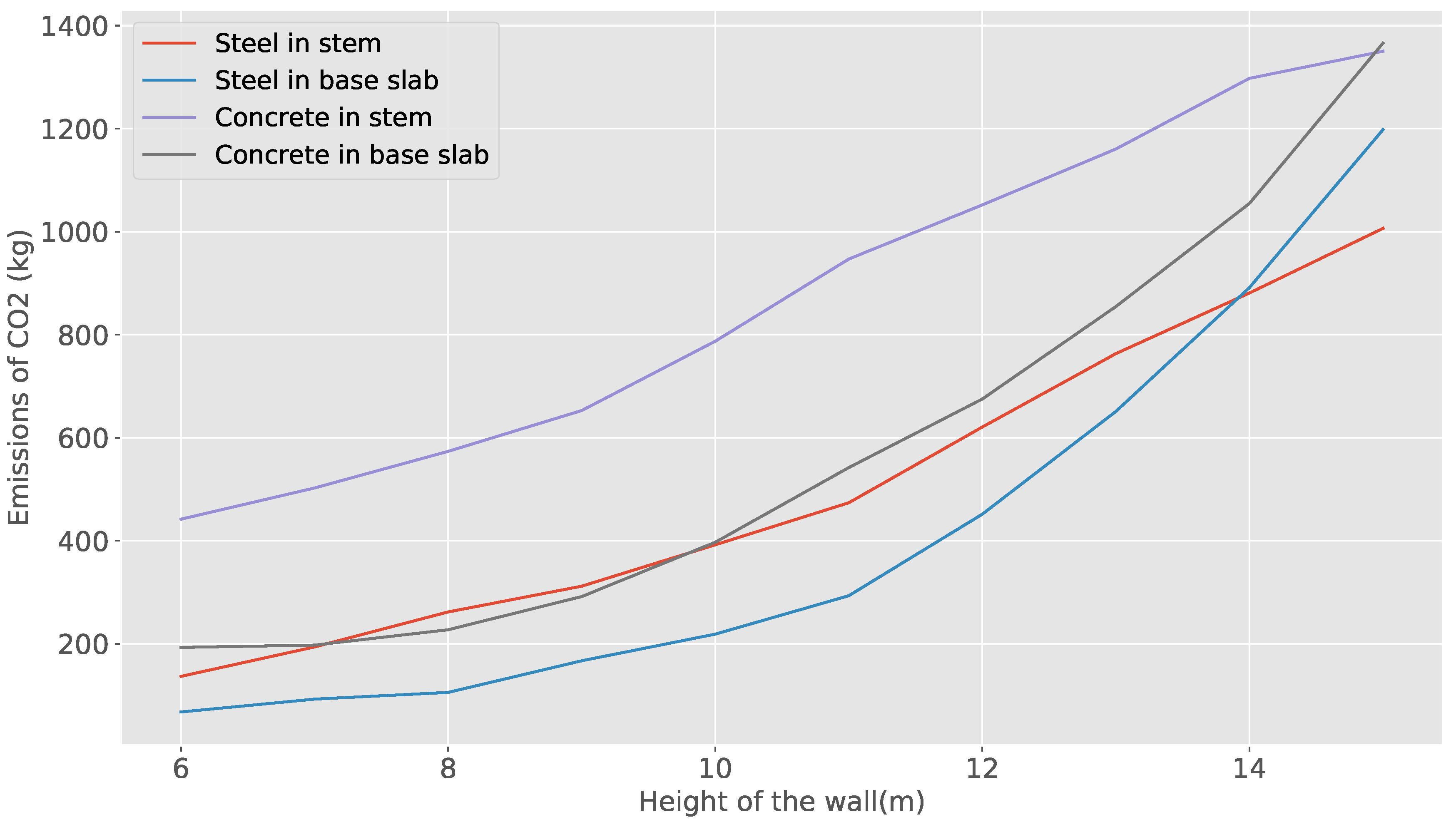
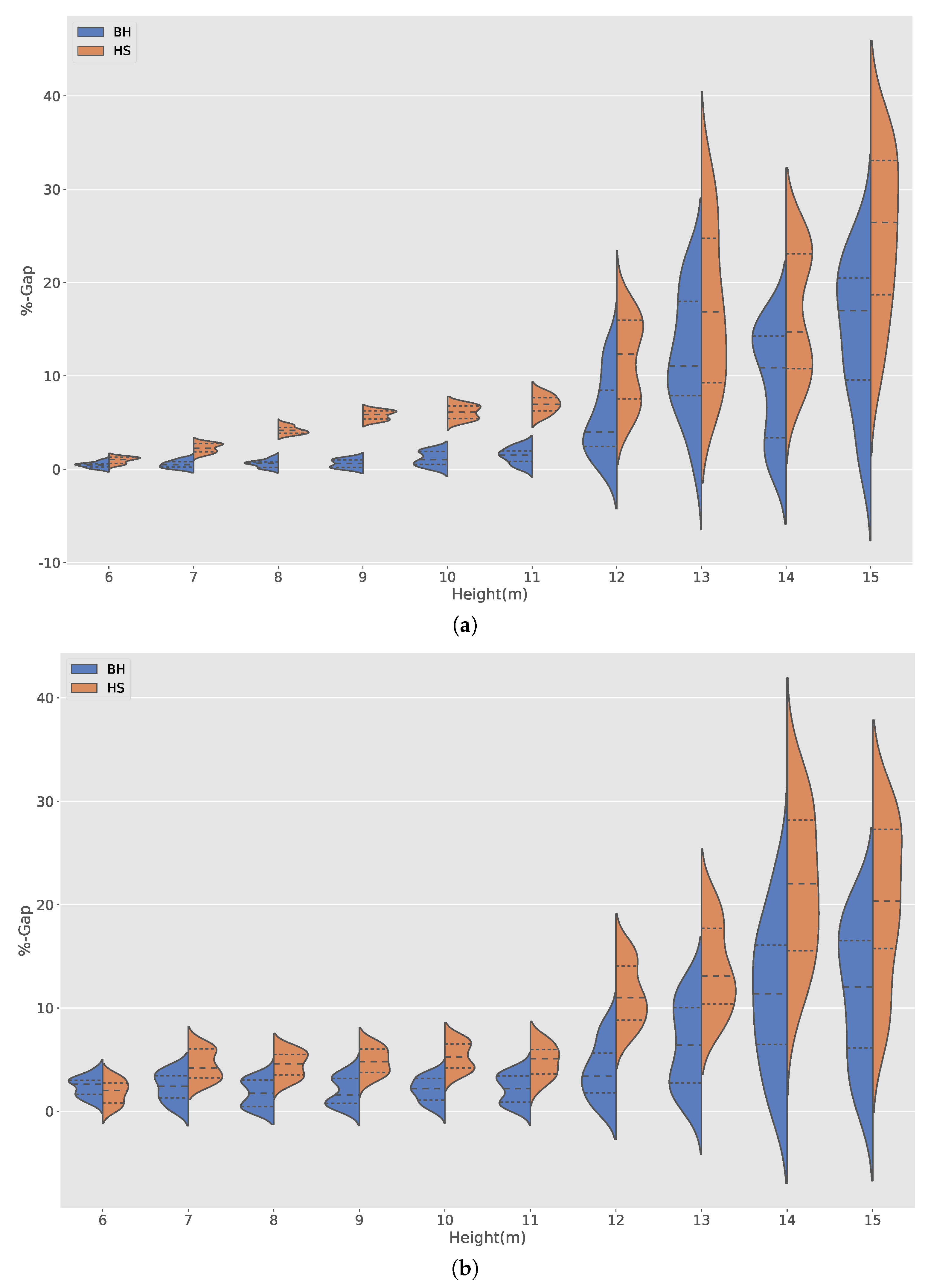
emission and structure costs do not deviate much from each other. As the wall grows, this difference increases, reaching a maximum at 11 m, where the emission deviates 6.16% and the cost 7.49%. When we analyze the main cause of this difference, it is found that it is related to the use of steel and cement. Solutions that minimize emissions prefer to use more concrete and less steel than those that optimize cost. Regarding the design variables, for optimal solutions, most of the values are very similar in both optimizations, with the exception of the variable of distance between buttresses, whose emission optimization value is always less than that obtained from cost optimization. For high heights (15 m), there is an inversion between the toe and heel length variables. As a result of the second analysis, in both optimizations and for the different wall heights, the concrete and the resulting steel in all cases are the C25/30 and BS500. When analyzing the dispersion results of the solutions for the different heights of the wall, it is observed that the dispersion of the solutions (Figure 11a,b) increases. This increase is considerable from the height of 12 m onwards. The above is an indication that our optimization problem is becoming more difficult as the height of the wall increases. This is consistent with the fact that at higher heights, it is more difficult to obtain stability of the wall concerning overturning and sliding. Finally, when we compare BH with HS, we observe that as we increase the height, BH performs better than HS, arriving at the height of 14 m at a difference of 4.67% in favor of BH in the optimization of emissions and 4.74% in cost minimization.
As a new line of research, it is interesting to explore robust optimization. Consider the optimization of the wall, but incorporating different values of some of the design variables within the optimization, as well as edge conditions, such as natural disasters. This makes the optimization problem much more difficult to address. Aiming at the latter, hybrid techniques can be used where metaheuristic algorithms are integrated with machine learning [46,47] techniques in order to improve the quality and convergence time of the solutions. This allows the tackling of more difficult problems, such as robust optimization in reasonable execution times.

Author Contributions

Conceptualization, V.Y., J.V.M. and J.G.; methodology, V.Y., J.V.M. and J.G.; software, J.V.M. and J.G.; validation, V.Y., J.V.M. and J.G.; formal analysis, V.Y.; investigation, J.V.M. and J.G.; data curation, J.V.M.; writing–original draft preparation, J.G.; writing–review and editing, V.Y., J.V.M. and J.G.;funding acquisition, V.Y. and J.G. All authors have read and agreed to the published version of the manuscript.

Funding

The authors acknowledge the financial support of the financial support of the Spanish Ministry of Economy and Competitiveness, along with FEDER funding (Project: BIA2017-85098-R) to the first and second authors, and the Grant CONICYT/FONDECYT/INICIACION/11180056 to the third author.

Conflicts of Interest

The authors declare no conflict of interest.

References

  1. Frangopol, D.M. Life-cycle performance, management, and optimisation of structural systems under uncertainty: Accomplishments and challenges. Struct. Infrast. Eng. 2011, 7, 389–413. [Google Scholar] [CrossRef]
  2. Ramesh, T.; Prakash, R.; Shukla, K.K. Life cycle energy analysis of buildings: An overview. Energy Build. 2010, 42, 1592–1600. [Google Scholar] [CrossRef]
  3. Boesch, M.E.; Hellweg, S. Identifying improvement potentials in cement production with life cycle assessment. Environ. Sci. Technol. 2010, 44, 9143–9149. [Google Scholar] [CrossRef]
  4. Serpell, A.; Kort, J.; Vera, S. Awareness, actions, drivers and barriers of sustainable construction in Chile. Technol. Econ. Dev. Econ. 2013, 19, 272–288. [Google Scholar] [CrossRef] [Green Version]
  5. Yusof, N.A.; Abidin, N.Z.; Zailani, S.H.M.; Govindan, K.; Iranmanesh, M. Linking the environmental practice of construction firms and the environmental behaviour of practitioners in construction projects. J. Clean. Prod. 2016, 121, 64–71. [Google Scholar] [CrossRef]
  6. Wang, T.; Lee, I.S.; Kendall, A.; Harvey, J.; Lee, E.B.; Kim, C. Life cycle energy consumption and GHG emission from pavement rehabilitation with different rolling resistance. J. Clean. Prod. 2012, 33, 86–96. [Google Scholar] [CrossRef]
  7. Wang, E.; Shen, Z. A hybrid Data Quality Indicator and statistical method for improving uncertainty analysis in LCA of complex system—Application to the whole-building embodied energy analysis. J. Clean. Prod. 2013, 43, 166–173. [Google Scholar] [CrossRef]
  8. Barandica, J.M.; Fernandez-Sanchez, G.; Berzosa, A.; Delgado, J.A.; Acosta, F.J. Applying life cycle thinking to reduce greenhouse gas emissions from road projects. J. Clean. Prod. 2013, 57, 79–91. [Google Scholar] [CrossRef]
  9. Aguado, A.; Caño, A.D.; de la Cruz, M.P.; Gomez, D.; Josa, A. Sustainability assessment of concrete structures within the Spanish structural concrete code. J. Constr. Eng. Manag. 2012, 138, 268–276. [Google Scholar] [CrossRef]
  10. Molina-Moreno, F.; García-Segura, T.; Martí, J.V.; Yepes, V. Optimization of counterfort retaining walls using hybrid harmony search algorithms. Eng. Struct. 2017, 134, 205–216. [Google Scholar] [CrossRef]
  11. Yepes, V.; Martí, J.V.; García-Segura, T. Cost and CO2 emission optimization of precast–prestressed concrete U-beam road bridges by a hybrid glowworm swarm algorithm. Autom. Constr. 2015, 49, 123–134. [Google Scholar] [CrossRef]
  12. Worrell, E.; Price, L.; Martin, N.; Hendriks, C.; Meida, L.O. Carbon dioxide emissions from the global cement industry. Ann. Rev. Energy Environ. 2001, 26, 303–329. [Google Scholar] [CrossRef]
  13. Molina-Moreno, F.; Martí, J.V.; Yepes, V. Carbon embodied optimization for buttressed earth-retaining walls: Implications for low-carbon conceptual designs. J. Clean. Prod. 2017, 164, 872–884. [Google Scholar] [CrossRef]
  14. Yepes, V.; Gonzalez-Vidosa, F.; Alcala, J.; Villalba, P. CO2-optimization design of reinforced concrete retaining walls based on a VNS-threshold acceptance strategy. J. Comput. Civ. Eng. 2012, 26, 378–386. [Google Scholar] [CrossRef] [Green Version]
  15. Yoon, Y.C.; Kim, K.H.; Lee, S.H.; Yeo, D. Sustainable design for reinforced concrete columns through embodied energy and CO2 emission optimization. Energy Build. 2018, 174, 44–53. [Google Scholar] [CrossRef]
  16. Sierra, L.A.; Pellicer, E.; Yepes, V. Social sustainability in the life cycle of Chilean public infrastructure. J. Constr. Eng. Manag. 2016, 142, 05015020. [Google Scholar] [CrossRef] [Green Version]
  17. Sierra, L.A.; Yepes, V.; García-Segura, T.; Pellicer, E. Bayesian network method for decision-making about the social sustainability of infrastructure projects. J. Clean. Prod. 2018, 176, 521–534. [Google Scholar] [CrossRef]
  18. Moayyeri, N.; Gharehbaghi, S.; Plevris, V. Cost-Based Optimum Design of Reinforced Concrete Retaining Walls Considering Different Methods of Bearing Capacity Computation. Mathematics 2019, 7, 1232. [Google Scholar] [CrossRef] [Green Version]
  19. Pons, J.J.; Penadés-Plà, V.; Yepes, V.; Martí, J.V. Life cycle assessment of earth-retaining walls: An environmental comparison. J. Clean. Prod. 2018, 192, 411–420. [Google Scholar] [CrossRef]
  20. Zastrow, P.; Molina-Moreno, F.; García-Segura, T.; Martí, J.V.; Yepes, V. Life cycle assessment of cost-optimized buttress earth-retaining walls: A parametric study. J. Clean. Prod. 2017, 140, 1037–1048. [Google Scholar] [CrossRef]
  21. Lee, D.; Kang, G.; Nam, C.; Cho, H.; Kang, K.I. Stochastic Analysis of Embodied Carbon Dioxide Emissions Considering Variability of Construction Sites. Sustainability 2019, 11, 4215. [Google Scholar] [CrossRef] [Green Version]
  22. Amirkhani, S.; Bahadori-Jahromi, A.; Mylona, A.; Godfrey, P.; Cook, D. Impact of low-e window films on energy consumption and CO2 emissions of an existing UK hotel building. Sustainability 2019, 11, 4265. [Google Scholar] [CrossRef] [Green Version]
  23. Lu, K.; Jiang, X.; Tam, V.W.; Li, M.; Wang, H.; Xia, B.; Chen, Q. Development of a Carbon Emissions Analysis Framework Using Building Information Modeling and Life Cycle Assessment for the Construction of Hospital Projects. Sustainability 2019, 11, 6274. [Google Scholar] [CrossRef] [Green Version]
  24. De Medeiros, G.F.; Kripka, M. Optimization of reinforced concrete columns according to different environmental impact assessment parameters. Eng. Struct. 2014, 59, 185–194. [Google Scholar] [CrossRef]
  25. Hussain, K.; Salleh, M.N.M.; Cheng, S.; Shi, Y. Metaheuristic research: A comprehensive survey. Artif. Intell. Rev. 2019, 52, 2191–2233. [Google Scholar] [CrossRef] [Green Version]
  26. Bozorg-Haddad, O. (Ed.) Advanced Optimization by Nature-Inspired Algorithms; Springer: Singapore, 2018. [Google Scholar]
  27. Geem, Z.W.; Kim, J.H.; Loganathan, G.V. A new heuristic optimization algorithm: Harmony search. Simulation 2001, 76, 60–68. [Google Scholar] [CrossRef]
  28. Kirkpatrick, S.; Gelatt, C.D.; Vecchi, M.P. Optimization by simulated annealing. Science 1983, 220, 671–680. [Google Scholar] [CrossRef]
  29. Cerny, V. Thermodynamical approach to the traveling salesman problem: An efficient simulation algorithm. J. Optim. Theory Appl. 1985, 45, 41–51. [Google Scholar] [CrossRef]
  30. Carbonell, A.; González-Vidosa, F.; Yepes, V. Design of reinforced concrete road vaults by heuristic optimization. Adv. Eng. Softw. 2011, 42, 151–159. [Google Scholar] [CrossRef]
  31. Zavadskas, E.K.; Antucheviciene, J.; Vilutiene, T.; Adeli, H. Sustainable decision-making in civil engineering, construction and building technology. Sustainability 2018, 10, 14. [Google Scholar] [CrossRef] [Green Version]
  32. Shi, X.; Wu, L.; Meng, X. A new optimization model for the sustainable development: Quadratic knapsack problem with conflict graphs. Sustainability 2017, 9, 236. [Google Scholar] [CrossRef] [Green Version]
  33. Sierra, L.A.; Yepes, V.; Pellicer, E. A review of multi-criteria assessment of the social sustainability of infrastructures. J. Clean. Prod. 2018, 187, 496–513. [Google Scholar] [CrossRef]
  34. García, J.; Moraga, P.; Valenzuela, M.; Crawford, B.; Soto, R.; Pinto, H.; Pena, A.; Altimiras, F.; Astroga, G. A Db-Scan Binarization Algorithm Applied to Matrix Covering Problems. Comput. Intell. Neurosci. 2019, 2019, 16. [Google Scholar] [CrossRef] [PubMed] [Green Version]
  35. García, J.; Crawford, B.; Soto, R.; Astorga, G. A clustering algorithm applied to the binarization of swarm intelligence continuous metaheuristics. Swarm Evol. Comput. 2019, 44, 646–664. [Google Scholar] [CrossRef]
  36. García, J.; Crawford, B.; Soto, R.; Astorga, G. A percentile transition ranking algorithm applied to binarization of continuous swarm intelligence metaheuristics. In Proceedings of the International Conference on Soft Computing and Data Mining, Johor, Malaysia, 6–8 February 2018; pp. 3–13. [Google Scholar]
  37. Yepes, V.; Alcala, J.; Perea, C.; González-Vidosa, F. A parametric study of optimum earth-retaining walls by simulated annealing. Eng. Struct. 2008, 30, 821–830. [Google Scholar] [CrossRef]
  38. García-Segura, T.; Yepes, V.; Alcalá, J. Life-cycle greenhouse gas emissions of blended cement concrete including carbonation and durability. Int. J. Life Cycle Assessment 2014, 19, 3–12. [Google Scholar] [CrossRef]
  39. Ministerio de Fomento. EHE: Code of Structural Concrete; Ministerio de Fomento: Madrid, Spain, 2008.
  40. Ministerio de Fomento. CTE. DB-SE. Structural Safety: Foundations; Ministerio de Fomento: Madrid, Spain, 2007. (In Spanish)
  41. Huntington, W.C. Earth Pressures and Retaining Wall; John Wiley and Sons: New York, NY, USA, 1957. [Google Scholar]
  42. Calavera, J. Muros de Contención y Muros de Sótano; Intemac: Madrid, Spain, 2001. (In Spanish) [Google Scholar]
  43. CEB-FIB. Model Code. In Design Code; Thomas Telford Services Ltd.: London, UK, 2001. [Google Scholar]
  44. Hatamlou, A. Black hole: A new heuristic optimization approach for data clustering. Inf. Sci. 2013, 222, 175–184. [Google Scholar] [CrossRef]
  45. García-Segura, T.; Yepes, V.; Alcalá, J.; Pérez-López, E. Hybrid harmony search for sustainable design of post-tensioned concrete box-girder pedestrian bridges. Eng. Struct. 2015, 92, 112–122. [Google Scholar] [CrossRef]
  46. García, J.; Lalla-Ruiz, E.; Voß, S.; López Droguett, E. Enhancing a machine learning binarization framework by perturbation operators: Analysis on the multidimensional knapsack problem. Int. J. Mach. Learn. Cyber. 2020. [Google Scholar] [CrossRef]
  47. García, J.; Crawford, B.; Soto, R.; Castro, C.; Paredes, F. A k-means binarization framework applied to multidimensional knapsack problem. Appl. Intell. 2018, 48, 357–380. [Google Scholar] [CrossRef]
Figure 1. Set of reinforcement variables. Source: [10].
Sustainability 12 02767 g001
Figure 2. Buttressed wall. Cross-section of the floor. Source: [10].
Sustainability 12 02767 g002
Figure 3. Problem design parameters. Source: [10].
Sustainability 12 02767 g003
Figure 4. Variation and dispersion of best costs and CO 2 emissions by the height of the wall.
Sustainability 12 02767 g004
Figure 5. Variation and dispersion of average costs and CO 2 emissions by the height of the wall.
Sustainability 12 02767 g005
Figure 6. Geometric variables depending on the height of the wall.
Sustainability 12 02767 g006
Figure 7. Ratio of geometrical variables.
Sustainability 12 02767 g007
Figure 8. Emissions of concrete and steel in the stem and foundation for CO 2 optimization.
Sustainability 12 02767 g008
Figure 9. Ratio of concrete and steel variables.
Sustainability 12 02767 g009
Figure 10. Best solution comparison between BH and HS. (a) Cost (€); (b) Emissions (kg CO2 eq.).
Sustainability 12 02767 g010
Figure 11. Comparison between BH and HS results. (a) % Cost gap; (b) % Emissions gap.
Sustainability 12 02767 g011
Table 1. Unit breakdown by unit cost, emissions, and cost. Source: [10].
UnitCost (€)Emissions (CO 2 -eq)
kg steel B4000.563.02
kg steel B5000.582.82
m 3 of concrete in stem
C25/3056.66224.34
C30/3760.80224.94
C35/4565.32265.28
C40/5070.41265.28
C45/5575.22265.91
C50/6080.03265.95
m 2 stem formwork21.611.92
m 3 of backfill5.5628.79
m 3 of concrete in foundation
C25/3050.65224.34
C30/3754.79224.94
C35/4559.31265.28
C40/5064.40265.28
C45/5569.21265.91
C50/6074.02265.95
Table 2. Design variables. Source: [10].
VariablesLower BoundUpper BoundIncrementN of Values
cH/20H/55 cmf(H) 1
dH/5 cm2H/35 cmf(H) 1
b25 cm122.52.5 cm40
p20 cm61010 cm60
t20 cm90515 cm60
e c 25 cm122.52.5 cm40
f c k 25, 20, 25, 40, 45, 50 7
f y k 400, 500 2
A 1 to A 10 6, 8, 10, 12, 16, 20, 25, 32 8
1 steel rebar12 rebars2 rebars6
A 11 to A 12 6, 8, 10, 12, 16, 20, 25, 328
1 steel rebar4 rebars10 rebars7
1 Depending on height.
Table 3. Problem design parameter values.
Parameter Considered Value
Bearing capacity 0.3 MPa
Fill slope 0
Foundation depth, H2 2 m
Uniform load on top of the fill, γ 10 kN/m 2
Base-friction coefficient, μ tg 30
Wall-fill friction angle, δ 0
Safety coefficient:
against sliding, γ f s 1.5
against overturning, γ f o 1.8
for loading (EHE)Normal
of steel (ULS)1.15
of concrete (ULS)1.5
Ambient exposure IIa
Table 4. Analysis of cost and emission optimization performed by the black hole (BH).
Height (m)Opt. CostEmissionsCostOpt. EmissionsCost from OptimumEmissions from Optimum
6593127060712592.36%0.87%
7679145569414412.21%0.97%
8774170679516592.71%2.83%
9912204693019981.97%2.40%
1010962589113524783.56%4.48%
1113093249140730607.49%6.18%
1215333841160037164.37%3.36%
1317834602187644715.22%2.93%
1420525523216352915.41%4.38%
1523637116249167885.42%4.83%
Table 5. Optimal costs and emissions for concrete and steel variables.
Cost Emissions
Optimization Optimization
HeightSteel inSteel inConcrete inConcrete inSteel inSteel inConcrete inConcrete in
Stem (Kg)Base (Kg)Stem (m 3 )Base (m 3 )Stem (Kg)Base (Kg)Stem (m 3 )Base (m 3 )
653.2730.511.880.8648.4823.961.970.86
779.9145.902.130.8868.7332.802.240.88
8121.4840.392.381.0192.8137.422.551.01
9134.0666.032.751.30110.5559.202.911.30
10187.7498.093.161.78139.0477.533.511.77
11234.57156.613.702.37167.98103.984.212.41
12272.33197.824.173.02220.12160.134.693.01
13372.58293.644.803.78270.65230.855.163.80
14411.92365.275.134.63312.40316.095.774.69
15481.51503.155.875.58356.85424.826.026.09

