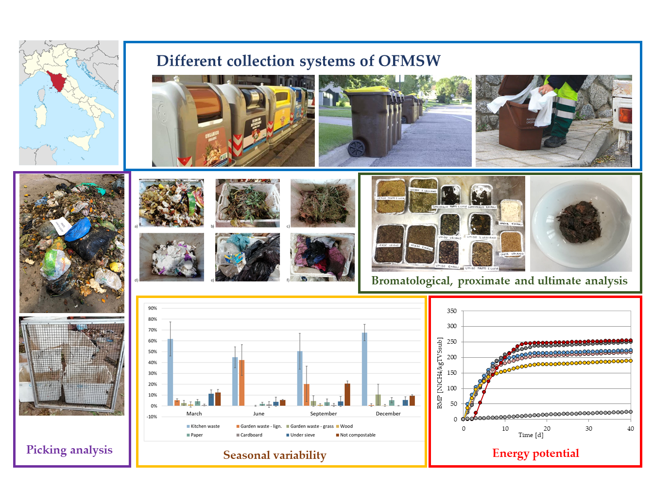
Bromatological, Proximate and Ultimate Analysis of OFMSW for Different Seasons and Collection Systems


Abstract
:
1. Introduction
2. Materials and Methods
2.1. Study Area Description
2.2. Sampling and Picking Analysis
2.3. Analysis of Dry and Volatile Matter
2.4. Proximate, Ultimate and Bromatological Analysis
2.5. Biochemical Methane Potential (BMP) Test
2.6. Statistical Analysis
3. Results and Discussion
3.1. Picking Analysis
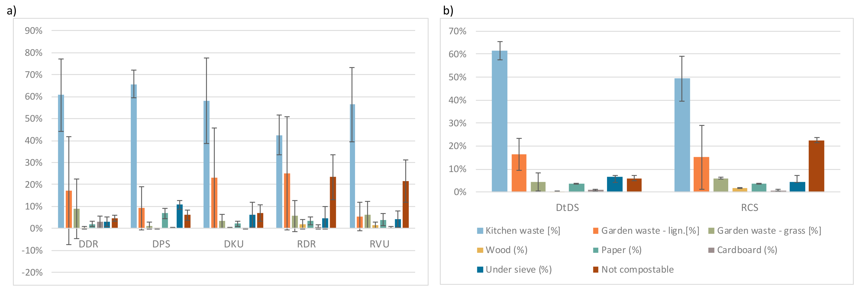
3.1.1. Variability due to Collection System
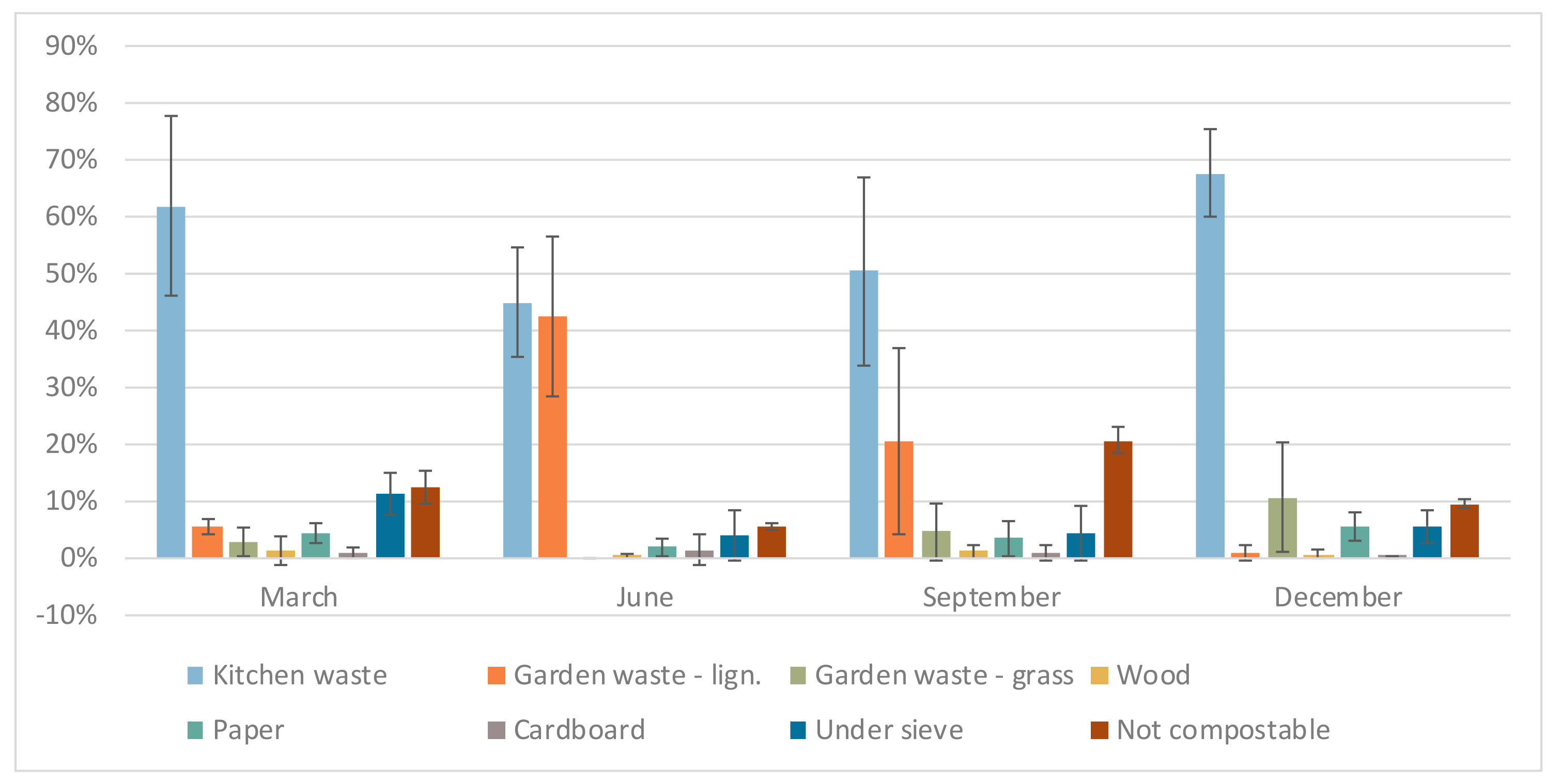
3.1.2. Seasonal Variability
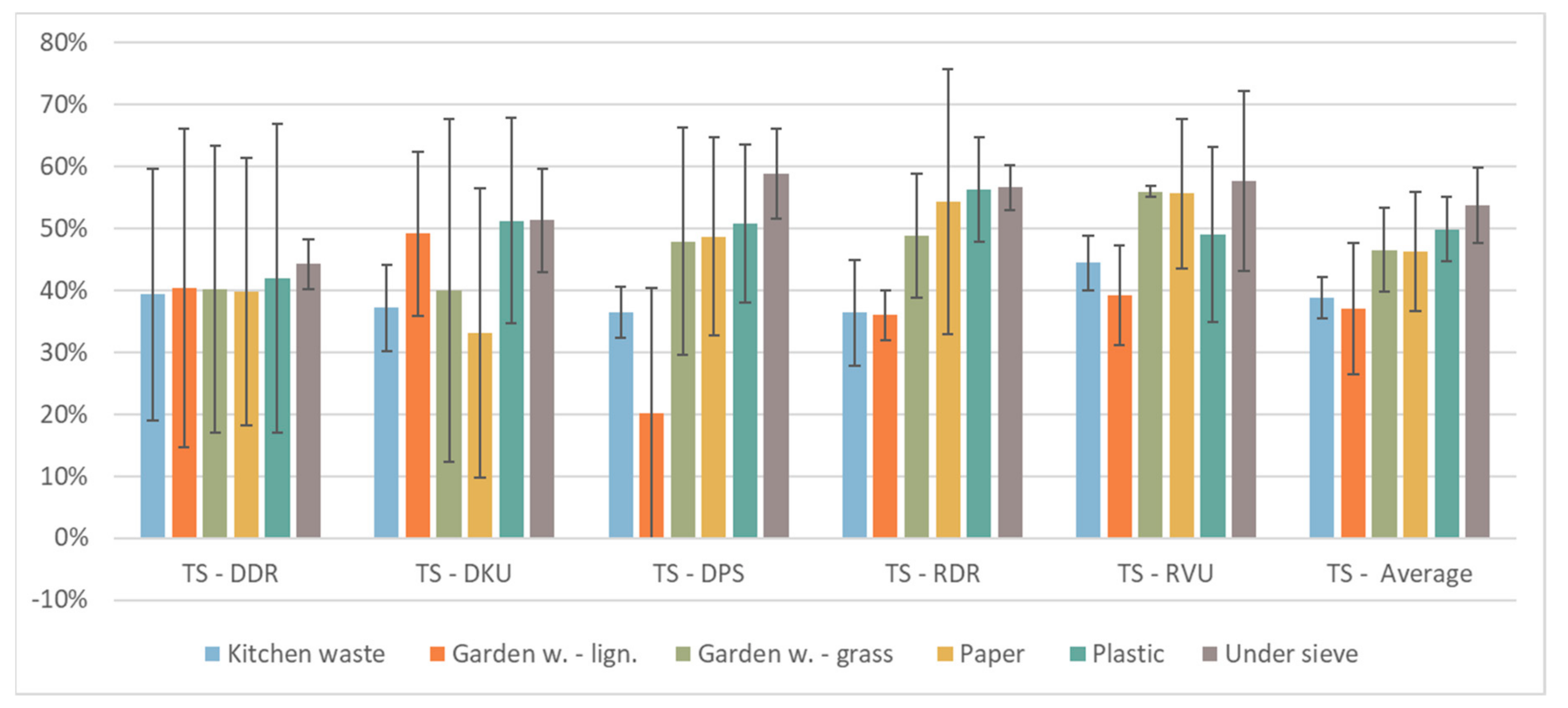
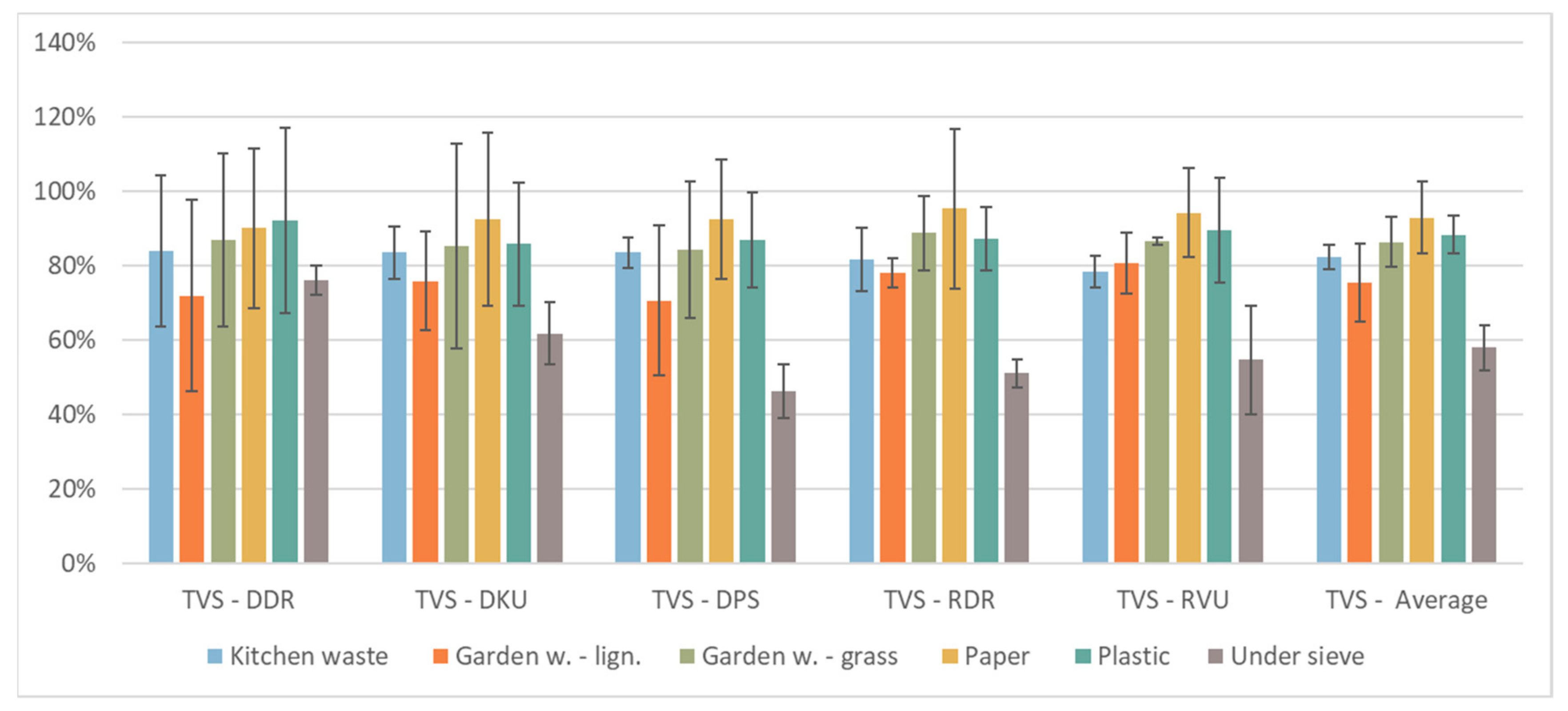
3.2. Dry and Volatile Matter
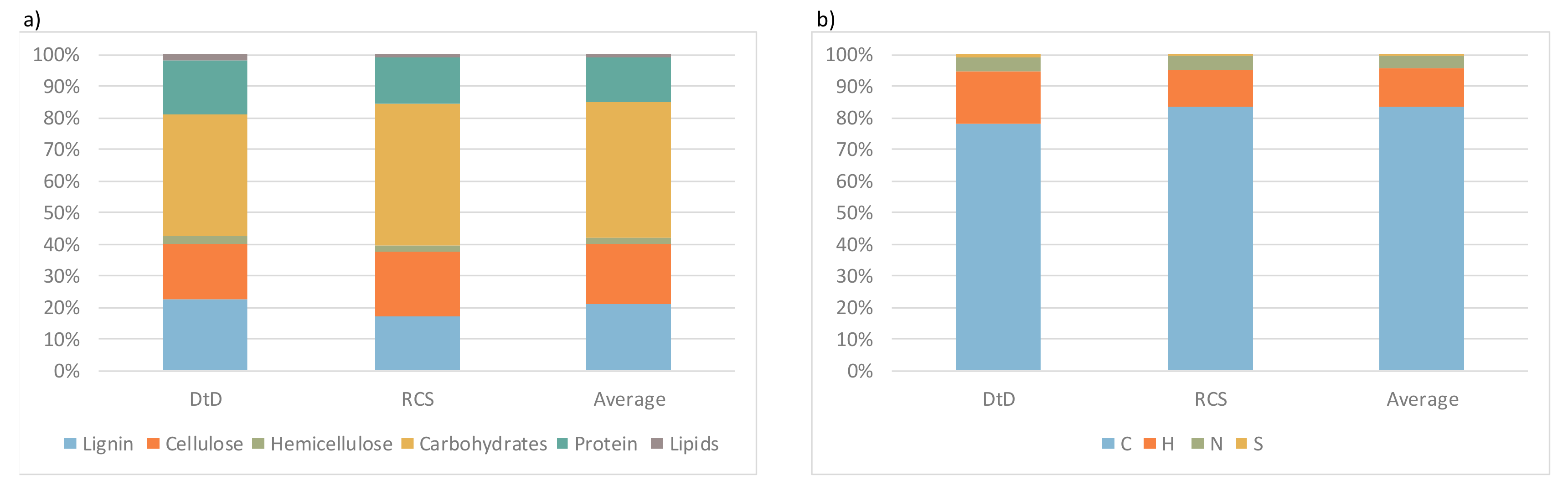
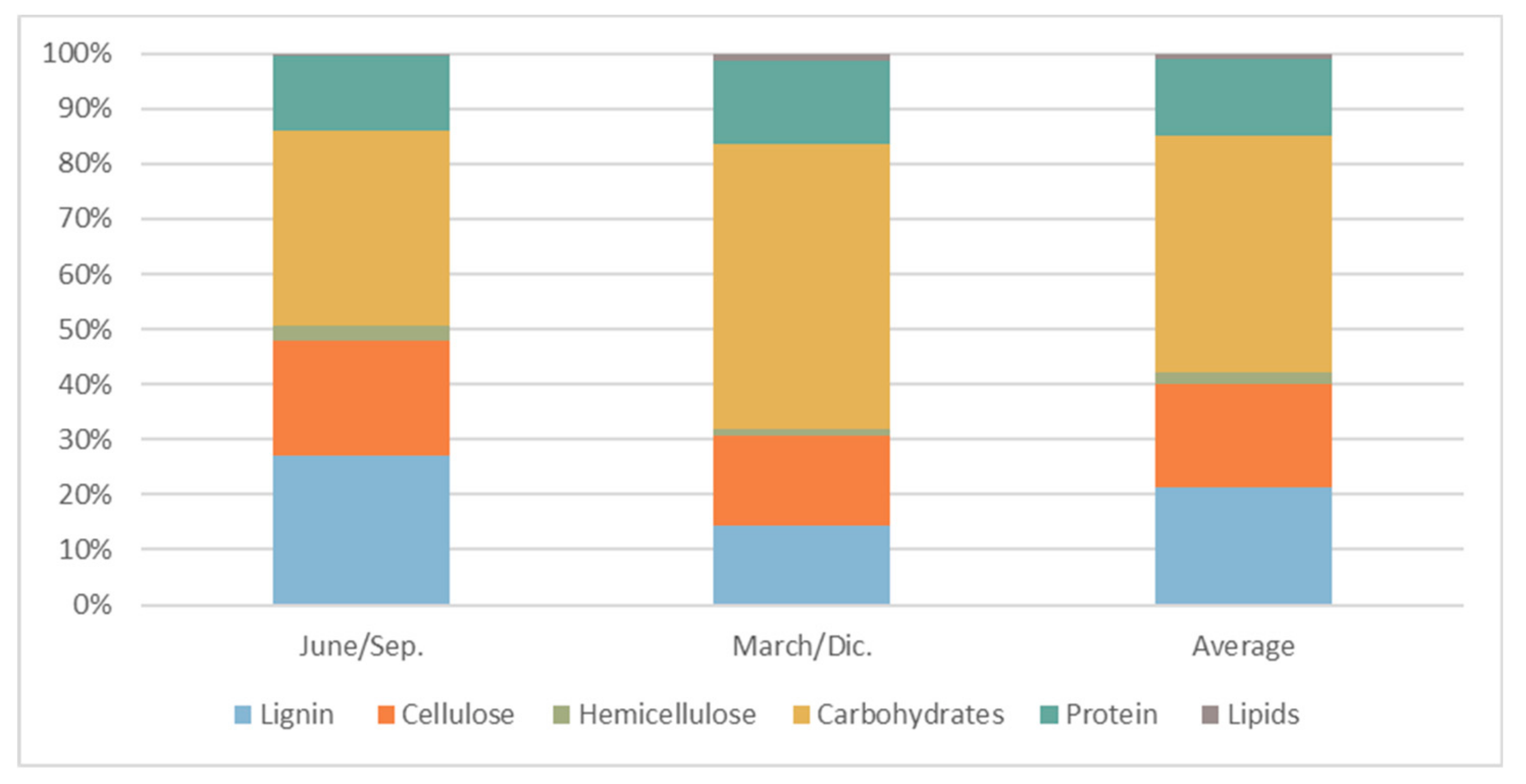
3.3. Proximate, Ultimate and Bromatological Analysis
3.3.1. Variability due to Collection Systems
3.3.2. Seasonal Variability
3.3.3. Nutritional Elements and Metals
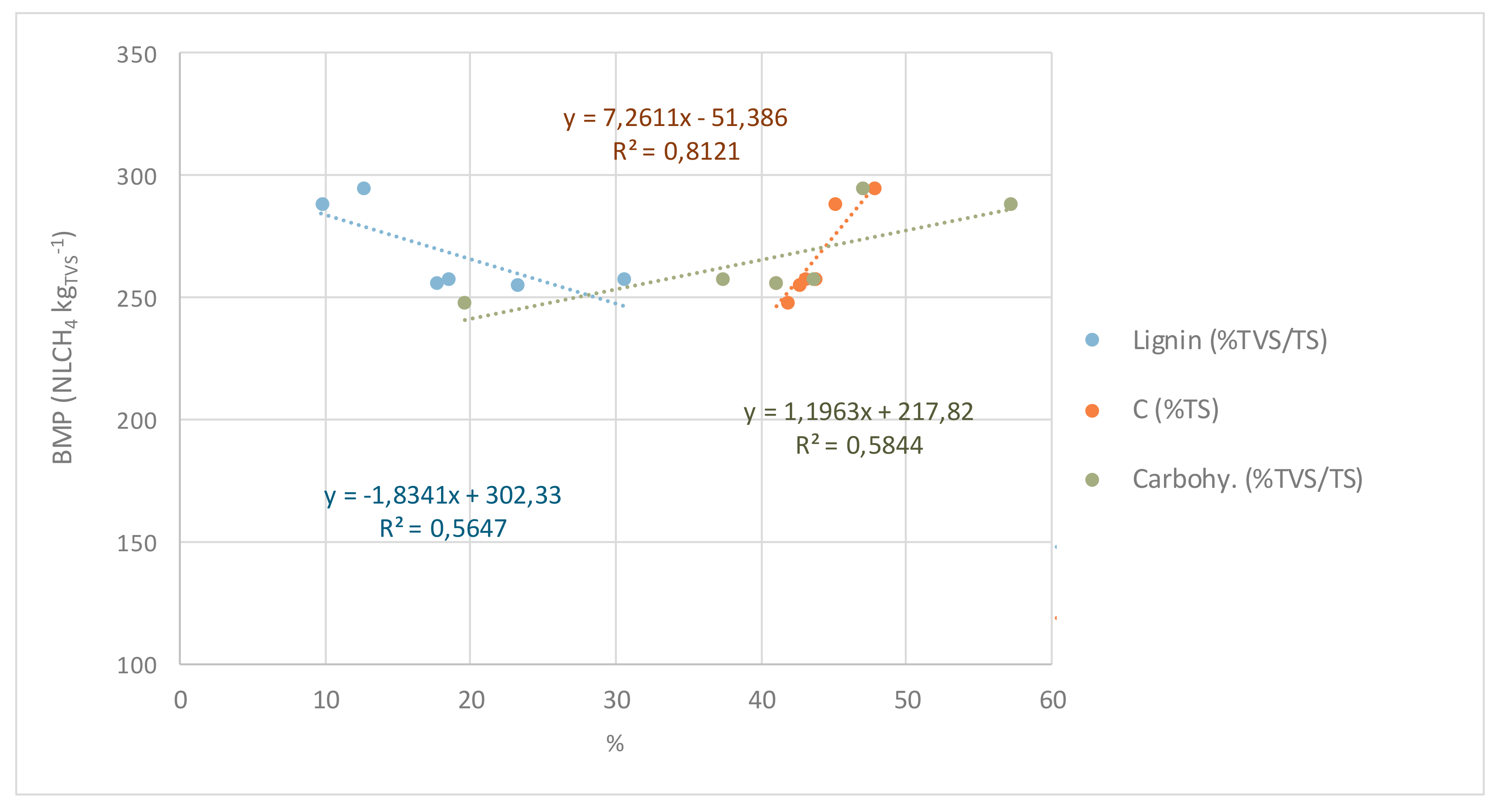
3.4. BMP Test
4. Conclusions
Author Contributions
Funding
Acknowledgments
Conflicts of Interest
Appendix A

| Fraction (%) | DDR | DPS | DKU | RDR | RVU | |||||
|---|---|---|---|---|---|---|---|---|---|---|
| Mean | St. Dev. | Mean | St. Dev. | Mean | St. Dev. | Mean | St. Dev. | Mean | St. Dev. | |
| Kitchen waste | 60.76% | 16.48% | 65.66% | 6.35% | 58.09% | 19.41% | 42.53% | 8.98% | 56.32% | 16.90% |
| Garden waste—lign. | 17.10% | 24.60% | 9.31% | 9.78% | 23.00% | 22.73% | 24.92% | 25.74% | 5.40% | 6.45% |
| Garden waste—grass | 8.98% | 13.60% | 1.30% | 1.74% | 3.29% | 3.25% | 5.66% | 6.99% | 6.23% | 6.25% |
| Wood | 0.36% | 0.53% | 0.05% | 0.08% | 0.33% | 0.38% | 1.81% | 2.26% | 1.52% | 1.37% |
| Paper | 2.10% | 1.09% | 6.91% | 2.30% | 2.22% | 1.23% | 3.43% | 1.86% | 4.03% | 2.64% |
| Cardboard | 2.95% | 2.73% | 0.22% | 0.20% | 0.07% | 0.08% | 0.66% | 1.00% | 0.45% | 0.31% |
| Textiles | 0.00% | 0.00% | 0.10% | 0.12% | 0.08% | 0.09% | 1.15% | 2.04% | 0.53% | 0.54% |
| Diapers | 0.12% | 0.11% | 0.17% | 0.26% | 0.37% | 0.74% | 2.18% | 2.65% | 2.46% | 1.25% |
| Plastic—Rigid | 1.92% | 3.26% | 2.00% | 3.88% | 1.50% | 2.86% | 2.38% | 3.26% | 0.53% | 0.63% |
| Plastic—Film | 1.67% | 1.63% | 2.75% | 2.58% | 2.86% | 3.06% | 1.96% | 1.33% | 4.09% | 1.46% |
| Plastic (non-packaging) | 0.04% | 0.07% | 0.00% | 0.00% | 0.11% | 0.17% | 0.13% | 0.26% | 0.77% | 0.92% |
| Inert | 0.00% | 0.00% | 0.05% | 0.11% | 0.02% | 0.04% | 0.17% | 0.34% | 0.56% | 0.78% |
| Metals | 0.11% | 0.13% | 0.04% | 0.04% | 1.11% | 1.94% | 0.20% | 0.20% | 0.45% | 0.13% |
| Glass | 0.10% | 0.17% | 0.02% | 0.04% | 0.08% | 0.10% | 0.71% | 0.39% | 1.06% | 0.42% |
| Polycoupled | 0.14% | 0.20% | 0.02% | 0.03% | 0.09% | 0.19% | 0.13% | 0.17% | 0.21% | 0.15% |
| Batteries | 0.00% | 0.00% | 0.01% | 0.01% | 0.00% | 0.00% | 0.00% | 0.00% | 0.00% | 0.00% |
| Drugs | 0.00% | 0.00% | 0.00% | 0.00% | 0.00% | 0.00% | 0.01% | 0.03% | 0.01% | 0.02% |
| Contribution errors | 0.59% | 1.02% | 1.07% | 1.34% | 0.94% | 1.25% | 14.31% | 11.03% | 10.98% | 7.39% |
| Under sieve | 3.06% | 2.22% | 10.86% | 2.01% | 6.31% | 5.79% | 4.82% | 4.96% | 4.30% | 3.66% |
| Not compostable (sum) | 4.70% | 1.29% | 5.68% | 2.36% | 6.70% | 3.76% | 16.17% | 10.30% | 21.66% | 9.56% |
| Fraction | March | June | September | December | ||||
|---|---|---|---|---|---|---|---|---|
| Mean | St. Dev. | Mean | St. Dev. | Mean | St. Dev. | Mean | St. Dev. | |
| Kitchen waste | 61.77% | 15.66% | 44.84% | 9.67% | 50.43% | 16.52% | 67.57% | 7.58% |
| Garden waste—lign. | 5.31% | 1.38% | 42.33% | 14.15% | 20.34% | 16.31% | 0.83% | 1.27% |
| Garden waste—grass | 2.79% | 2.40% | 0.00% | 0.00% | 4.58% | 4.91% | 10.51% | 9.61% |
| Wood | 1.34% | 2.45% | 0.26% | 0.47% | 1.07% | 1.16% | 0.54% | 0.78% |
| Paper | 4.30% | 1.78% | 1.91% | 1.51% | 3.44% | 3.06% | 5.32% | 2.44% |
| Cardboard | 0.78% | 0.95% | 1.35% | 2.70% | 0.91% | 1.44% | 0.18% | 0.19% |
| Textiles | 0.23% | 0.18% | 0.04% | 0.08% | 1.12% | 1.79% | 0.06% | 0.08% |
| Diapers | 0.62% | 0.85% | 0.33% | 0.53% | 2.32% | 2.66% | 0.64% | 0.66% |
| Plastic—Rigid | 0.33% | 0.37% | 0.08% | 0.15% | 5.30% | 3.10% | 0.54% | 0.59% |
| Plastic—Film | 1.87% | 1.07% | 3.50% | 0.79% | 0.70% | 1.55% | 4.53% | 2.06% |
| Plastic (non-packaging) | 0.10% | 0.20% | 0.09% | 0.18% | 0.49% | 0.77% | 0.03% | 0.05% |
| Inert | 0.25% | 0.30% | 0.00% | 0.00% | 0.33% | 0.63% | 0.00% | 0.00% |
| Metals | 0.21% | 0.17% | 1.00% | 2.01% | 0.23% | 0.17% | 0.21% | 0.21% |
| Glass | 0.40% | 0.47% | 0.18% | 0.28% | 0.53% | 0.51% | 0.35% | 0.63% |
| Polycoupled | 0.05% | 0.07% | 0.19% | 0.22% | 0.05% | 0.12% | 0.16% | 0.16% |
| Batteries | 0.00% | 0.00% | 0.00% | 0.00% | 0.00% | 0.00% | 0.01% | 0.01% |
| Drugs | 0.00% | 0.00% | 0.00% | 0.00% | 0.02% | 0.03% | 0.00% | 0.00% |
| Contribution errors | 8.39% | 9.99% | 0.00% | 0.00% | 9.52% | 8.52% | 2.95% | 2.54% |
| Under sieve | 11.27% | 3.54% | 3.90% | 4.26% | 4.28% | 4.66% | 5.58% | 2.94% |
| Not compostable (sum) | 12.44% | 2.81% | 5.41% | 0.57% | 20.62% | 2.40% | 9.47% | 0.85% |
| (mg/Kg) | DDR | DKU | DPS | RDR | RVU | |||||
|---|---|---|---|---|---|---|---|---|---|---|
| Mean | St. Dev. | Mean | St. Dev. | Mean | St. Dev. | Mean | St. Dev. | Mean | St. Dev. | |
| Nutritional elements | ||||||||||
| NH3 —N | 293.51 | 195.67 | 492.45 | 344.33 | 411.01 | 345.03 | 259.65 | 218.22 | 765.00 | 49.50 |
| Ca | 8255.28 | 7279.17 | 7183.31 | 6956.27 | 8012.96 | 6622.56 | 7411.93 | 5716.07 | 4925.00 | 49.50 |
| P | 584.38 | 97.55 | 806.94 | 135.21 | 630.93 | 85.87 | 667.54 | 58.71 | 729.50 | 262.34 |
| Na | 1305.26 | 929.93 | 1580.08 | 899.11 | 1510.42 | 1132.35 | 1335.00 | 692.15 | 1310.00 | 0.00 |
| K | 2260.91 | 241.60 | 2539.83 | 234.14 | 2259.53 | 179.31 | 2497.56 | 376.34 | 2115.00 | 7.07 |
| Fe | 764.25 | 512.97 | 3335.81 | 5051.71 | 576.69 | 330.21 | 585.28 | 412.97 | 257.00 | 197.99 |
| Mn | 50.11 | 36.39 | 185.97 | 283.11 | 28.89 | 11.90 | 45.82 | 17.04 | 13.50 | 2.12 |
| Mg | 768.38 | 409.05 | 844.96 | 813.70 | 873.41 | 283.79 | 663.13 | 279.00 | 945.00 | 770.75 |
| Mo | 1.83 | 0.30 | 1.00 | 0.40 | 1.43 | 0.51 | 1.35 | 0.47 | 1.50 | 0.71 |
| Zn | 13.45 | 7.68 | 218.06 | 401.31 | 13.67 | 6.24 | 18.29 | 7.03 | 10.50 | 4.95 |
| Metals | ||||||||||
| As | 0.70 | 0.52 | 0.55 | 0.52 | 0.33 | 0.45 | 0.33 | 0.45 | 0.10 | 0.00 |
| Al | 483.53 | 406.41 | 383.87 | 111.01 | 539.39 | 190.12 | 359.01 | 252.60 | 324.00 | 248.90 |
| Ba | 10.41 | 4.69 | 18.04 | 14.45 | 11.99 | 4.09 | 18.63 | 13.77 | 31.50 | 31.82 |
| Cr | 2.32 | 1.53 | 2.74 | 2.22 | 1.86 | 1.02 | 1.95 | 0.82 | 2.50 | 2.12 |
| Cd | 0.01 | 0.01 | 0.01 | 0.01 | 0.01 | 0.01 | 1.00 | 0.01 | 0.01 | 0.01 |
| Cu | 5.84 | 3.34 | 610.38 | 1206.42 | 6.82 | 2.95 | 6.90 | 2.43 | 3.50 | 0.71 |
| Ni | 2.52 | 1.83 | 3.51 | 2.09 | 1.78 | 1.02 | 3.61 | 3.35 | 0.75 | 0.35 |
| Pb | 1.69 | 1.19 | 1.76 | 0.98 | 3.04 | 2.62 | 3.81 | 3.02 | < 1 | |
| Hg | 0.5 | 0 | 5.625 | 10.25 | 0.5 | 0 | 0.5 | 0.00 | 0.50 | 0.00 |
| (mg/Kg) | March | June | September | December | Average | |||||
|---|---|---|---|---|---|---|---|---|---|---|
| Mean | St. Dev. | Mean | St. Dev. | Mean | St. Dev. | Mean | St. Dev. | Media | St. Dev. | |
| Nutritional elements | ||||||||||
| NH3—N | 772.25 | 230.02 | 461.00 | 31.72 | 176.75 | 170.55 | 284.60 | 257.16 | 423.65 | 260.26 |
| Ca | 4130.00 | 582.69 | 16,397.41 | 1050.55 | 4462.25 | 3011.12 | 6078.00 | 1134.87 | 7766.92 | 5816.24 |
| P | 821.75 | 89.18 | 644.70 | 9.14 | 591.00 | 119.90 | 618.00 | 43.98 | 668.86 | 104.26 |
| Na | 1572.50 | 562.75 | 2506.19 | 484.62 | 670.75 | 154.89 | 1048.00 | 217.99 | 1449.36 | 795.69 |
| K | 2145.00 | 189.82 | 2426.11 | 9.83 | 2459.00 | 455.99 | 2416.00 | 228.10 | 2361.53 | 145.51 |
| Fe | 285.50 | 130.44 | 1019.21 | 185.46 | 596.75 | 432.31 | 503.40 | 320.96 | 601.22 | 307.67 |
| Mn | 22.75 | 12.37 | 56.51 | 10.53 | 31.00 | 17.63 | 38.00 | 27.80 | 37.06 | 14.38 |
| Mg | 647.50 | 389.99 | 885.53 | 80.89 | 693.50 | 369.38 | 916.00 | 385.07 | 785.63 | 134.84 |
| Mo | 1.00 | 0.00 | 1.52 | 0.14 | 1.25 | 0.50 | 2.80 | 1.79 | 1.64 | 0.80 |
| Zn | 11.75 | 2.63 | 20.61 | 2.77 | 17.25 | 8.18 | 10.00 | 3.74 | 14.90 | 4.90 |
| Metals | ||||||||||
| As | 0.10 | 0.00 | 1.00 | 0.00 | 0.10 | 0.00 | 0.46 | 0.49 | 0.42 | 0.43 |
| Al | 350.25 | 214.84 | 442.16 | 76.45 | 332.50 | 327.75 | 545.60 | 229.97 | 417.63 | 97.92 |
| Ba | 34.25 | 18.71 | 12.73 | 1.94 | 14.50 | 7.77 | 10.50 | 1.91 | 17.99 | 10.96 |
| Cr | 1.50 | 0.58 | 2.04 | 0.28 | 2.75 | 2.36 | 2.60 | 1.52 | 2.22 | 0.57 |
| Cd | 0.01 | 0.01 | 0.01 | 0.01 | 0.01 | 0.01 | 0.01 | 0.01 | 0.01 | 0.01 |
| Cu | 5.00 | 1.15 | 9.48 | 0.14 | 6.50 | 2.65 | 4.00 | 1.41 | 6.25 | 2.39 |
| Ni | 0.88 | 0.25 | 3.92 | 0.55 | 3.38 | 3.25 | 1.40 | 0.89 | 2.39 | 1.48 |
| Pb | < 1 | 2.92 | 0.55 | 4.00 | 2.94 | 1.00 | 0.00 | 2.23 | 1.49 | |
| Hg | 0.50 | 0.00 | 0.50 | 0.00 | 0.50 | 0.00 | 0.50 | 0.00 | 0.50 | 0.00 |
References
- EUR-Lex-52010DC0235-EN. Available online: https://eur-lex.europa.eu/legal-content/EN/TXT/HTML/?uri=CELEX:52010DC0235&from=EN (accessed on 8 March 2020).
- Rapporto Rifiuti Urbani-Edizione 2019. Available online: http://www.isprambiente.gov.it/it/pubblicazioni/rapporti/rapporto-rifiuti-urbani-edizione-2019 (accessed on 8 March 2020).
- EUR-Lex-52015DC0614-EN-EUR-Lex. Available online: https://eur-lex.europa.eu/legal-content/EN/TXT/?uri=CELEX%3A52015DC0614 (accessed on 8 March 2020).
- Baldi, F.; Pecorini, I.; Iannelli, R. Comparison of single-stage and two-stage anaerobic co-digestion of food waste and activated sludge for hydrogen and methane production. Renew. Energy 2019, 143, 1755–1765. [Google Scholar] [CrossRef]
- Union, P.O. of the E. A Sustainable Bioeconomy for Europe: Strengthening the Connection between Economy, Society and the Environment: Updated Bioeconomy Strategy. Available online: https://op.europa.eu:443/en/publication-detail/-/publication/edace3e3-e189-11e8-b690-01aa75ed71a1/language-en (accessed on 6 February 2020).
- Demichelis, F.; Piovano, F.; Fiore, S. Biowaste Management in Italy: Challenges and Perspectives. Sustainability 2019, 11, 4213. [Google Scholar] [CrossRef] [Green Version]
- Tyagi, V.K.; Fdez-Güelfo, L.A.; Zhou, Y.; Álvarez-Gallego, C.J.; Garcia, L.I.R.; Ng, W.J. Anaerobic co-digestion of organic fraction of municipal solid waste (OFMSW): Progress and challenges. Renew. Sustain. Energy Rev. 2018, 93, 380–399. [Google Scholar] [CrossRef]
- Angelidaki, I.; Chen, X.; Cui, J.; Kaparaju, P.; Ellegaard, L. Thermophilic anaerobic digestion of source-sorted organic fraction of household municipal solid waste: Start-up procedure for continuously stirred tank reactor. Water Res. 2006, 40, 2621–2628. [Google Scholar] [CrossRef]
- Fernández-Rodríguez, J.; Pérez, M.; Romero, L.I. Comparison of mesophilic and thermophilic dry anaerobic digestion of OFMSW: Kinetic analysis. Chem. Eng. J. 2013, 232, 59–64. [Google Scholar] [CrossRef]
- Beggio, G.; Schievano, A.; Bonato, T.; Hennebert, P.; Pivato, A. Statistical analysis for the quality assessment of digestates from separately collected organic fraction of municipal solid waste (OFMSW) and agro-industrial feedstock. Should input feedstock to anaerobic digestion determine the legal status of digestate? Waste Manag. 2019, 87, 546–558. [Google Scholar] [CrossRef]
- Zhang, R.; Elmashad, H.; Hartman, K.; Wang, F.; Liu, G.; Choate, C.; Gamble, P. Characterization of food waste as feedstock for anaerobic digestion. Bioresour. Technol. 2007, 98, 929–935. [Google Scholar] [CrossRef]
- Melts, I.; Normak, A.; Nurk, L.; Heinsoo, K. Chemical characteristics of biomass from nature conservation management for methane production. Bioresour. Technol. 2014, 167, 226–231. [Google Scholar] [CrossRef]
- Campuzano, R.; González-Martínez, S. Characteristics of the organic fraction of municipal solid waste and methane production: A review. Waste Manag. 2016, 54, 3–12. [Google Scholar] [CrossRef]
- Xu, F.; Wang, Z.-W.; Li, Y. Predicting the methane yield of lignocellulosic biomass in mesophilic solid-state anaerobic digestion based on feedstock characteristics and process parameters. Bioresour. Technol. 2014, 173, 168–176. [Google Scholar] [CrossRef]
- Long, G.; Liu, S.; Xu, G.; Wong, S.-W.; Chen, H.; Xiao, B. A Perforation-Erosion Model for Hydraulic-Fracturing Applications. SPE Prod. Oper. 2018, 33, 770–783. [Google Scholar] [CrossRef]
- Xiao, B.; Wang, W.; Zhang, X.; Long, G.; Fan, J.; Chen, H.; Deng, L. A novel fractal solution for permeability and Kozeny-Carman constant of fibrous porous media made up of solid particles and porous fibers. Powder Technol. 2019, 349, 92–98. [Google Scholar] [CrossRef]
- Xiao, B.; Zhang, X.; Jiang, G.; Long, G.; Wang, W.; Zhang, Y.; Liu, G. KOZENY–CARMAN CONSTANT FOR GAS FLOW THROUGH FIBROUS POROUS MEDIA BY FRACTAL-MONTE CARLO SIMULATIONS. Fractals 2019, 27, 1950062. [Google Scholar] [CrossRef]
- Fisgativa, H.; Tremier, A.; Dabert, P. Characterizing the variability of food waste quality: A need for efficient valorisation through anaerobic digestion. Waste Manag. 2016, 50, 264–274. [Google Scholar] [CrossRef] [PubMed]
- Pecorini, I.; Baldi, F.; Albini, E.; Galoppi, G.; Bacchi, D.; Valle, A.D.; Baldi, A.; Bianchini, A.; Figini, A.; Rossi, P.; et al. Hydrogen production from food waste using biochemical hydrogen potential test. Procedia Environ. Sci. Eng. Manag. 2017, 4, 155–162. [Google Scholar]
- Bernstad, A.; la Cour Jansen, J. Separate collection of household food waste for anaerobic degradation—Comparison of different techniques from a systems perspective. Waste Manag. 2012, 32, 806–815. [Google Scholar] [CrossRef]
- Browne, J.D.; Murphy, J.D. Assessment of the resource associated with biomethane from food waste. Appl. Energy 2013, 104, 170–177. [Google Scholar] [CrossRef]
- Hla, S.S.; Roberts, D. Characterisation of chemical composition and energy content of green waste and municipal solid waste from Greater Brisbane, Australia. Waste Manag. 2015, 41, 12–19. [Google Scholar] [CrossRef]
- Azam, M.; Jahromy, S.S.; Raza, W.; Raza, N.; Lee, S.S.; Kim, K.-H.; Winter, F. Status, characterization, and potential utilization of municipal solid waste as renewable energy source: Lahore case study in Pakistan. Environ. Int. 2020, 134, 105291. [Google Scholar] [CrossRef]
- Pecorini, I.; Bacchi, D.; Albini, E.; Baldi, F.; Galoppi, G.; Rossi, P.; Paoli, P.; Ferrari, L.; Carnevale, E.A.; Peruzzini, M.; et al. The bio2energy project: Bioenergy, biofuels and bioproducts from municipal solid waste and sludge. In Proceedings of the 25th European Biomass Conference and Exhibition, Stockholm, Sweden, 12–15 June 2017; Volume 2017, pp. 70–77. [Google Scholar]
- Morlok, J.; Schoenberger, H.; Styles, D.; Galvez-Martos, J.-L.; Zeschmar-Lahl, B. The Impact of Pay-As-You-Throw Schemes on Municipal Solid Waste Management: The Exemplar Case of the County of Aschaffenburg, Germany. Resources 2017, 6, 8. [Google Scholar] [CrossRef]
- Gallardo, A.; Prades, M.; Bovea, M.D.; Colomer, F.J. Separate Collection Systems for Urban Waste (UW). In Management of Organic Waste; Kumar, S., Ed.; InTech: London, UK, 2012. [Google Scholar]
- Nappi, P.; Valenzano, F.; Consiglio, M.; Piemonte, A. Analisi merceologica dei rifiuti urbani Rassegna di metodologie e definizione di una metodica di riferimento. Available online: https://www.arpal.liguria.it/files/rifiuti/ANPA_Merceologia.pdf (accessed on 7 March 2020).
- Hansen, T.L.; la Cour Jansen, J.; Spliid, H.; Davidsson, Å.; Christensen, T.H. Composition of source-sorted municipal organic waste collected in Danish cities. Waste Manag. 2007, 27, 510–518. [Google Scholar] [CrossRef] [PubMed]
- Pecorini, I.; Iannelli, R. Characterization of Excavated Waste of Different Ages in View of Multiple Resource Recovery in Landfill Mining. Sustainability 2020, 12, 1780. [Google Scholar] [CrossRef] [Green Version]
- Pecorini, I.; Bacchi, D.; Iannelli, R. Biodrying of the Light Fraction from Anaerobic Digestion Pretreatment in Order to Increase the Total Recovery Rate. Processes 2020, 8, 276. [Google Scholar] [CrossRef] [Green Version]
- Metodi di Analisi del Compost. Available online: http://www.isprambiente.gov.it/it/pubblicazioni/manuali-e-linee-guida/metodi-di-analisi-del-compost (accessed on 1 March 2020).
- Pecorini, I.; Baldi, F.; Carnevale, E.A.; Corti, A. Biochemical methane potential tests of different autoclaved and microwaved lignocellulosic organic fractions of municipal solid waste. Waste Manag. 2016, 56, 143–150. [Google Scholar] [CrossRef] [PubMed]
- Naroznova, I.; Møller, J.; Scheutz, C. Characterisation of the biochemical methane potential (BMP) of individual material fractions in Danish source-separated organic household waste. Waste Manag. 2016, 50, 39–48. [Google Scholar] [CrossRef] [Green Version]
- Angelidaki, I.; Alves, M.; Bolzonella, D.; Borzacconi, L.; Campos, J.L.; Guwy, A.J.; Kalyuzhnyi, S.; Jenicek, P.; van Lier, J.B. Defining the biomethane potential (BMP) of solid organic wastes and energy crops: A proposed protocol for batch assays. Water Sci. Technol. 2009, 59, 927–934. [Google Scholar] [CrossRef] [PubMed] [Green Version]
- Pecorini, I.; Baldi, F.; Iannelli, R. Biochemical Hydrogen Potential Tests Using Different Inocula. Sustainability 2019, 11, 622. [Google Scholar] [CrossRef] [Green Version]
- Pecorini, I.; Olivieri, T.; Bacchi, D.; Paradisi, A.; Lombardi, L.; Corti, A.; Carnevale, E. Evaluation of gas production in a industrial anaerobic digester by means of biochemical methane potential of organic municipal solid waste components. In Proceedings of the 25th International Conference on Efficiency, Cost, Optimization, Simulation and Environmental Impact of Energy Systems, Perugia, Italy, 26–29 June 2012; Volume 5, pp. 173–184. [Google Scholar]
- Pecorini, I.; Baldi, F.; Carnevale, E.A.; Corti, A. Enhancement of methane production of microwaved pretreated biowaste at different enthalpies. In Proceedings of the 28th International Conference on Efficiency, Cost, Optimization, Simulation and Environmental Impact of Energy Systems, ECOS 2015, Pau, France, 29 June–3 July 2015. [Google Scholar]
- Baldi, F.; Iannelli, R.; Pecorini, I.; Polettini, A.; Pomi, R.; Rossi, A. Influence of the pH control strategy and reactor volume on batch fermentative hydrogen production from the organic fraction of municipal solid waste. Waste Manag. Res. 2019, 37, 478–485. [Google Scholar] [CrossRef] [Green Version]
- Cesaro, A.; Russo, L.; Belgiorno, V. Combined anaerobic/aerobic treatment of OFMSW: Performance evaluation using mass balances. Chem. Eng. J. 2015, 267, 16–24. [Google Scholar] [CrossRef]
- Alvarez, M.D.; Sans, R.; Garrido, N.; Torres, A. Factors that affect the quality of the bio-waste fraction of selectively collected solid waste in Catalonia. Waste Manag. 2008, 28, 359–366. [Google Scholar] [CrossRef]
- López, M.; Soliva, M.; Martínez-Farré, F.X.; Fernández, M.; Huerta-Pujol, O. Evaluation of MSW organic fraction for composting: Separate collection or mechanical sorting. Resour. Conserv. Recycl. 2010, 54, 222–228. [Google Scholar] [CrossRef]
- Chen, Y.; Cheng, J.J.; Creamer, K.S. Inhibition of anaerobic digestion process: A review. Bioresour. Technol. 2008, 99, 4044–4064. [Google Scholar] [CrossRef] [PubMed]
- Iacovidou, E.; Ohandja, D.-G.; Voulvoulis, N. Food waste co-digestion with sewage sludge—Realising its potential in the UK. J. Environ. Manag. 2012, 112, 267–274. [Google Scholar] [CrossRef] [PubMed]
- APAT Digestione Anaerobica Della Frazione Organica dei Rifiuti Solidi. Available online: http://www.isprambiente.gov.it/it/pubblicazioni/manuali-e-linee-guida/digestione-anaerobica-della-frazione-organica-dei (accessed on 7 March 2020).


| Acronym | System | Type | Areas | Residents | Type of Container | Description | |
|---|---|---|---|---|---|---|---|
| DDR | Door-to-door (DtDS) | Door-to-door collection system | Rural | 10.183 (Density 298.53 res./km2) | bin (25 L) | Houses with garden. | 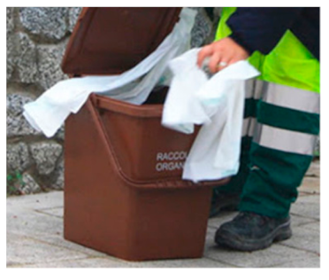 |
| DPS | Door-to-door collection system with pay-as-you- throw | Semi-urban | 48.795 (Density 783.48 res./km2) | bin (25 L) | Presence of small houses with garden and apartment buildings with 2 floors. | ||
| DKU | Curbside collection system | Urban | 195.089 (Density 2004 res./km2) | bin (90 L) | Residential neighborhood. Apartments from 2 to 5 floors. | 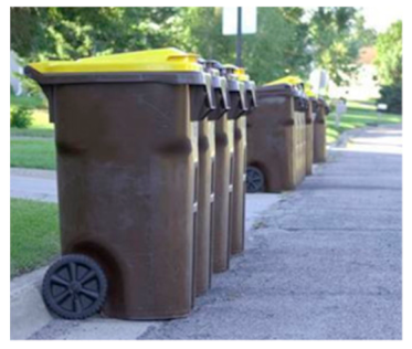 | |
| RDR | Road containers (RCS) | Dropoff points system | Rural | 17,129 (Density 158.85 res./km2) | containers (3000 L) | Small apartment buildings of 2 floors and houses with garden. | 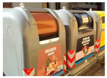 |
| RVU | Drop-off points system volume-based | Urban | 379,563 (Density 3709.57 res./km2) | containers (3000 L) | City with apartment buildings from 2 to 7 floors. | ||
| Parameter | Method | Parameter | Method |
|---|---|---|---|
| pH | EPA 9045D 2004 | Ammonia | UNI 10780:1998 App. J |
| Conductivity | APAT CNR IRSA 2030 Man 29 2003 | Calcium (Ca); Aluminum (Al) | UNI EN 13657:2004 + UNI EN ISO 11885:2009 |
| Total Organic Carbon (TOC) | UNI 10780:1998 App. E | ||
| C/N ratio | UNI EN 13137:2002 + UNI EN | Phosphorus (P) Sodium (Na) | EPA 3050B 1996 + EPA 6010D 2014 |
| 15407:2011 | Potassium (K) | UNI 10780:1998 App. B | |
| Hydrogen (H) | DM 13/09/1999 SO GU n° 248 | Iron (Fe) | EPA 3050B 1996 + EPA 6010D 2014 |
| 21/10/1999 Met VII.1 | Magnesium (Mg) | UNI EN 13657:2004 + UNI EN ISO 11885:2009 | |
| Carbon (C) | DM 13/09/1999 SO GU n° 248 | Manganese (Mn) | UNI EN 13657:2004 + UNI EN ISO 11885:2009 |
| 21/10/1999 Met VII.3 | Molybdenum (Mo) | UNI EN 13657:2004 + UNI EN ISO 11885:2009 | |
| Nitrogen (N) | UNI EN 15407:2011 | ||
| Sulphur (S) | EPA 5050 1994 + EPA 9056° 2007 | Nickel (Ni) | UNI 10780:1998 App. B |
| Lignin, Cellulose, Hemicellulose, Carbohydrates | POM 017 Rev. 0 2011 | Lead (Pb) Mercury (Hg) | UNI 10780:1998 App. B |
| Protein | ISTISAN 1996/34 pag.13 | Copper (Cu) | UNI 10780:1998 App. B |
| Lipids | CNR IRSA Met 21 Q 64 vol 3 1998 | Arsenic (As) | UNI 10780:1998 App. B |
| ID | TS (%) | TS (%)—Calculated from Individual Sample | TVS/TS (%) | TVS/TS (%)—Calculated from Individual Sample | ||||
|---|---|---|---|---|---|---|---|---|
| Mean | st.d. | mean | st.d. | mean | st.d. | mean | st.d. | |
| DDR* | 41.2% | 10.0% | 40.1% | 2.3% | 87.2% | 2.0% | 82.6% | 6.3% |
| DKU* | 43.5% | 6.4% | 43.6% | 2.6% | 85.6% | 6.7% | 82.6% | 4.9% |
| DPS* | 47.7% | 9.7% | 41.4% | 7.3% | 81.5% | 7.5% | 80.3% | 4.3% |
| RDR* | 38.1% | 5.4% | 42.9% | 4.7% | 72.5% | 20.1% | 82.9% | 8.5% |
| RVU* | 44.3% | 6.6% | 42.6% | 6.3% | 92.4% | 3.0% | 74.4% | 6.1% |
| March** | 42.8% | 0.2% | 44.8% | 1.8% | 88.6% | 7.3% | 79.3% | 7.8% |
| June** | 40.1% | 7.4% | 42.5% | 6.1% | 72.3% | 16.7% | 86.2% | 3.9% |
| September** | 40.8% | 4.9% | 42.2% | 2.4% | 83.5% | 2.5% | 82.8% | 5.6% |
| December** | 48.0% | 12.2% | 40.5% | 6.3% | 88.6% | 3.5% | 79.3% | 7.8% |
| Annual average | 42.9% | 3.6% | 42.5% | 1.8% | 83.3% | 7.7% | 81.9% | 3.3% |
| Analysis | DDR | DKU | DPS | RDR | RVU | ||||||
|---|---|---|---|---|---|---|---|---|---|---|---|
| Unit | Mean | St. Dev. | Mean | St. Dev. | Mean | St. Dev. | Mean | St. Dev. | Mean | St. Dev. | |
| Proximate | |||||||||||
| pH | - | 4.33 | 0.78 | 4.39 | 0.72 | 4.62 | 0.62 | 5.04 | 0.74 | 3.93 | 0.11 |
| Conductivity | μS/cm | 4120.88 | 1346.83 | 3681.55 | 2513.19 | 5308.10 | 908.79 | 4745.54 | 811.27 | 5025.00 | 657.61 |
| Ash | % | 6.64 | 4.44 | 63.99 | 115.38 | 6.41 | 2.34 | 7.23 | 3.76 | 3.66 | 0.49 |
| TS | % | 30.57 | 8.77 | 31.35 | 18.34 | 31.98 | 5.74 | 40.18 | 12.58 | 31.00 | 11.03 |
| TVS | % | 23.93 | 4.35 | 32.50 | 5.55 | 25.56 | 5.56 | 32.95 | 12.16 | 27.35 | 10.54 |
| TOC | % | 20.21 | 4.61 | 27.92 | 2.84 | 22.46 | 4.36 | 29.21 | 11.75 | 25.20 | 9.48 |
| Ultimate | |||||||||||
| C | %TS | 43.06 | 6.55 | 43.75 | 5.26 | 42.65 | 2.43 | 44.63 | 4.98 | 47.80 | 2.38 |
| H | %TS | 5.98 | 1.25 | 15.38 | 18.36 | 6.07 | 0.48 | 6.32 | 0.88 | 6.63 | 0.11 |
| N | %TS | 2.16 | 0.47 | 3.03 | 2.04 | 2.07 | 0.26 | 2.21 | 0.51 | 2.54 | 0.31 |
| S | %TS | 0.17 | 0.10 | 0.72 | 1.10 | 0.18 | 0.11 | 0.14 | 0.07 | 0.14 | 0.06 |
| C/N | 23.12 | 2.79 | 15.46 | 10.26 | 22.43 | 4.59 | 24.83 | 6.12 | 19.00 | 2.83 | |
| Bromatological | |||||||||||
| Lignin | %TVS | 30.58 | 13.91 | 18.45 | 8.52 | 23.21 | 15.21 | 21.87 | 12.19 | 12.64 | 2.03 |
| Cellulose | %TVS | 18.55 | 6.09 | 17.88 | 7.28 | 20.31 | 4.40 | 21.32 | 5.61 | 19.07 | 7.87 |
| Hemicellulose | %TVS | 2.63 | 2.61 | 3.55 | 2.86 | 1.87 | 1.16 | 2.33 | 1.38 | 1.60 | 0.57 |
| Carbohydrates | %TVS | 37.36 | 22.90 | 43.57 | 24.32 | 42.10 | 19.10 | 42.28 | 20.49 | 46.98 | 12.40 |
| Protein | %TVS | 15.97 | 0.82 | 23.54 | 19.84 | 15.10 | 1.08 | 14.56 | 2.79 | 14.58 | 2.14 |
| Lipids | %TVS | 1.41 | 0.97 | 3.58 | 6.11 | 1.07 | 0.73 | 0.82 | 0.62 | 1.15 | 0.57 |
| Analysis | March | June | September | December | Average | ||||||
|---|---|---|---|---|---|---|---|---|---|---|---|
| Unit | Mean | St. Dev. | Mean | St. Dev. | Mean | St. Dev. | Mean | St. Dev. | Media | St. Dev. | |
| Proximate | |||||||||||
| pH | - | 3.91 | 0.07 | 5.21 | 0.01 | 4.53 | 0.74 | 4.40 | 0.74 | 4.51 | 0.54 |
| Conductivity | /cm | 5197.50 | 310.20 | 5752.35 | 485.73 | 3775.00 | 606.88 | 4658.00 | 576.47 | 4845.71 | 842.10 |
| Ash | % | 5.33 | 2.22 | 10.11 | 0.61 | 3.95 | 2.70 | 5.43 | 2.23 | 6.21 | 2.69 |
| TS | % | 43.93 | 9.22 | 37.76 | 1.66 | 32.00 | 9.06 | 27.30 | 3.44 | 35.25 | 7.20 |
| TVS | % | 38.60 | 7.15 | 27.65 | 1.05 | 28.05 | 8.92 | 21.87 | 2.09 | 29.04 | 6.97 |
| TOC | % | 34.40 | 7.85 | 24.47 | 0.94 | 22.78 | 5.89 | 19.12 | 1.14 | 25.19 | 6.53 |
| Ultimate | |||||||||||
| C | %TS | 45.07 | 3.20 | 48.87 | 1.90 | 41.83 | 2.42 | 41.00 | 3.82 | 44.19 | 3.58 |
| H | %TS | 6.45 | 0.25 | 6.97 | 0.20 | 5.99 | 0.54 | 5.56 | 0.77 | 6.24 | 0.60 |
| N | %TS | 2.01 | 0.35 | 2.33 | 0.02 | 2.15 | 0.60 | 2.24 | 0.41 | 2.18 | 0.14 |
| S | %TS | 0.10 | 0.02 | 0.28 | 0.05 | 0.15 | 0.02 | 0.11 | 0.04 | 0.16 | 0.08 |
| C/N | 25.00 | 4.03 | 20.92 | 0.55 | 26.63 | 4.37 | 18.60 | 1.95 | 22.79 | 3.68 | |
| Bromatological | |||||||||||
| Lignin | %TVS/TS | 9.73 | 2.08 | 22.47 | 2.26 | 38.98 | 9.44 | 17.67 | 3.33 | 22.21 | 12.35 |
| Cellulose | %TVS/TS | 13.38 | 4.34 | 23.45 | 0.68 | 23.56 | 3.72 | 17.21 | 4.67 | 19.40 | 4.99 |
| Hemicellulose | %TVS/TS | 1.70 | 0.53 | 2.13 | 0.54 | 3.95 | 1.38 | 0.74 | 0.68 | 2.13 | 1.35 |
| Carbohydrates | %TVS/TS | 57.11 | 7.33 | 60.79 | 0.01 | 19.60 | 7.58 | 41.04 | 7.37 | 44.63 | 18.76 |
| Protein | %TVS/TS | 14.15 | 2.11 | 15.21 | 0.59 | 15.13 | 3.32 | 14.31 | 1.54 | 14.70 | 0.55 |
| Lipids | %TVS/TS | 0.76 | 0.44 | 0.55 | 0.08 | 0.68 | 0.41 | 1.98 | 0.36 | 0.99 | 0.67 |
| BMP (NLCH4 kgTVS−1) | GS (Nm3tOFMSW−1) | CH4 (%v/v) | |||||||
|---|---|---|---|---|---|---|---|---|---|
| Mean | St. Dev. | p Value | Mean | St. Dev. | p Value | Mean | St. Dev. | p Value | |
| DDR | 257.27a | 18.91 | 0.34 | 134.63a | 17.05 | 0.16 | 55.87a | 1.44 | 0.66 |
| DKU | 257.05a | 17.15 | 159.35a | 22.06 | 55.78a | 1.09 | |||
| DPS | 255.25a | 24.42 | 138.90a | 20.82 | 55.35a | 0.09 | |||
| RDR | 231.70b | 44.63 | 0.13 | 155.78b | 47.46 | 0.72 | 54.69b | 0.74 | 0.69 |
| RVU | 294.35b | 14.07 | 141.85b | 21.71 | 54.30b | 1.70 | |||
| March | 288.50c,e | 12.36 | 0.02 | 172.73c | 27.13 | 0.10 | 55.33c | 0.13 | 0.37 |
| June | 228.08d | 27.85 | 146.48c | 11.83 | 55.95c | 1.87 | |||
| September | 248.05d | 21.89 | 146.70c | 34.61 | 55.24c | 0.19 | |||
| December | 255.60d,e | 27.63 | 128.02c | 19.95 | 54.68c | 0.91 | |||
| Average | 255.06 | 25.14 | 148.48 | 18.38 | 55.30 | 0.52 | |||
© 2020 by the authors. Licensee MDPI, Basel, Switzerland. This article is an open access article distributed under the terms and conditions of the Creative Commons Attribution (CC BY) license (http://creativecommons.org/licenses/by/4.0/).
Share and Cite
Pecorini, I.; Rossi, E.; Iannelli, R. Bromatological, Proximate and Ultimate Analysis of OFMSW for Different Seasons and Collection Systems. Sustainability 2020, 12, 2639. https://doi.org/10.3390/su12072639
Pecorini I, Rossi E, Iannelli R. Bromatological, Proximate and Ultimate Analysis of OFMSW for Different Seasons and Collection Systems. Sustainability. 2020; 12(7):2639. https://doi.org/10.3390/su12072639
Chicago/Turabian StylePecorini, Isabella, Elena Rossi, and Renato Iannelli. 2020. "Bromatological, Proximate and Ultimate Analysis of OFMSW for Different Seasons and Collection Systems" Sustainability 12, no. 7: 2639. https://doi.org/10.3390/su12072639
APA StylePecorini, I., Rossi, E., & Iannelli, R. (2020). Bromatological, Proximate and Ultimate Analysis of OFMSW for Different Seasons and Collection Systems. Sustainability, 12(7), 2639. https://doi.org/10.3390/su12072639