Article

Joint Optimization of Routes and Container Fleets to Design Sustainable Intermodal Chains in Chile

by
Alba Martínez-López
* and
Manuel Chica
Department of Mechanical Engineering, University of Las Palmas de Gran Canaria, 35017 Las Palmas, Spain
*
Author to whom correspondence should be addressed.
Sustainability 2020, 12(6), 2221; https://doi.org/10.3390/su12062221
Submission received: 16 February 2020 / Revised: 6 March 2020 / Accepted: 7 March 2020 / Published: 12 March 2020
(This article belongs to the Special Issue Sustainable Maritime Transportation Management and Policies)

Abstract

:
This paper introduces a decision support tool for sustainable intermodal chains with seaborne transport, in which the optimization of a multi-objective model enables conflicting objectives to be handled simultaneously. Through the assessment of ‘door-to-door’ transport in terms of costs, time, and environmental impact, the most suitable maritime route and the optimized fleet are jointly calculated to maximize the opportunities for success of intermodal chains versus trucking. The resolution of the model through NSGA-II algorithms permits to obtain Pareto fronts that offer groups of optimized solutions. This is not only useful to make decisions in the short term, but also to establish long-term strategies through assessment of the frontiers’ behavior obtained when a sensitivity analysis is undertaken. Thus, consequences of transport policies on intermodal performance can be analyzed. A real-life case is studied to test the usefulness of the model. From the application case, not only the most suitable Motorway of the Seas with their optimized fleets are identified for Chile, but also significant general findings are provided for both policy makers and heads of ports to promote the intermodal option regardless of their geographical locations.

1. Introduction

With the intention of finding alternatives to the congestion problems on European roads, the European Union (EU) has boosted its transport policy based on the idea of intermodality as the most sustainable solution for ‘door-to-door’ transport. Due to this sustainability, Short Sea Shipping (SSS) has attracted special attention as one of the most interesting trunk hauls (stretches for consolidation cargo) for intermodal chains. Far from being a regional aim, the development of SSS has gained international interest. Thus, whereas, in the European Union (White Paper: European Transport Policy for 2010), the SSS concept was developing towards motorways of the sea (MoS; from 2001, the SSS along with the intermodal services and the ports being affected by the establishment of intermodal chains), Canada and the United States signed a Memorandum of Cooperation on Sharing Short Sea Shipping Information and Experience in 2003 [1]. The SSS concept that is integrated into intermodal chains has been widely studied in the last decade in broader contexts than the European Union and from different perspectives: in South America [2,3], North America [4], Australia [5] and Asia [6,7], among others; consequently, MoS is currently an offshore concept and has been largely attended.
Despite the considerable interest in the establishment of MoS, a consensus exists about the limited success of their operation [8]. Over the last decade, different authors have highlighted possible reasons for this circumstance, among others:
  • Despite the numerous studies aiming to improve intermodal chains with a maritime leg, most of them have focused on the identification of the most suitable maritime routes to replace road transport with intermodal chains. These studies have considered two relevant initial assumptions: the technical and the operative features of the fleets are fixed [9]. Most of the vessels considered have been Ro-Ro vessels (Roll-on, Roll-off vessels; this refers to vessels with rolled cargo) with previous activity on other maritime routes. As a result, many studies have finally adapted the maritime routes to the current fleet instead adapting the fleets to the most interesting routes.
  • Increasing discussion about the ‘green label’ of the Short Sea Shipping has also taken place in recent years [10,11,12]. A significant normative imbalance in terms of pollutant emissions damages the competitiveness of SSS in relation to road transport in the EU; the quick normative development in land transport demanding higher pollutant restrictions [13] along with the low impact of the economies of scale in SSS with small and quick vessels [10,14], have led to the intermodal chains not being as sustainable as was accepted several years ago [7].
Albeit highly convenient for the social interest, the responsibility for articulating suitable intermodal chains with a seaborne haul currently lies with private companies. These companies compromise the environmental performance of the whole chain by taking decisions about the technical and operative features of the fleets and their operative localization. However, as expected, the ship operators are uniquely focused on the ship selection by optimizing their commercial activity on the haul on which they operate [15].
This reality, along with the complexity of modeling the whole chain, has meant that very few papers have tackled SSS fleet optimization by taking into account the competitiveness of whole chains from the loader standpoint. This approach involves that the competitiveness evaluation must be carried out through a comparison with the unimodal alternative. The Artificial Intelligence (AI) is a very useful tool to solve complex decision problems; however, most of the studies in this domain have focused again, on just one haul (often on port operations or scheduling problems). Into this reduced group, scare researchers have developed multi-objective models able to offer decision support tools based on what-if analyses addressed to the intermodal competitiveness. The research gap is even broader when considering the absence of models able to analyze the joint effect of technical and operative features of the fleets and routes on the intermodal performance.
Thus, partial approaches to the intermodality, combined with the simplification of the problem to mono-objective models, have limited the exploration of intermodal competitiveness. Consequently, even though noteworthy breakthroughs exist in this field, very few publications have offered decision support tools based on a global perspective of ‘door-to-door’ transport. Among them, syncromodality projects [16] stand out by offering useful decision-making tools for stakeholders, which are able to optimize results through collaboration among transport modes. This tool is especially useful to reach compromise solutions, since the modal shift is integrated to handle conflicting objectives simultaneously (times, costs, sustainability, etc.) [16].
The previous lack is especially significant when taking into account the low success level reached by MoS and the wide acceptance that the correct assessment of transport competitiveness must consider not only fleet features but also cargo characteristics and geographical aspects that highly determine the modal choice and the success of the MoS [17].
To contribute to filling this knowledge gap, this paper introduces a multi-objective mathematical model to assess a whole ‘many-to-many’ intermodal chain (that is, many possible origins and many possible destinations) by operating with optimized fleets for the seaborne hauls [18] in terms of costs, time, and the environmental impact in relation to the unimodal alternative. The model presented in this paper is the result of the integration of successive optimization models for vessels into intermodal chains that were previously developed in the EU context [19,20]. In such a way, the current model offers wider capacities through its ability to suggest sustainable solutions for fleets and maritime routes in different frameworks, beyond the EU context, by overcoming partial attachments.
The mathematical model provided in this paper assumes as optimization variables the technical and operative features of the container fleets and the geographical inputs of the routes at the same time. Thus, the resolution of the model permits to reach global results for sustainable intermodal chains beyond seaborne, since the optimization of the fleet for every maritime stretch is based on the competitiveness results of the whole transport network.
Thus, with the nodes of a particular transport network being known (possible origins or destinations of the freight on land), the proposed model is able to suggest the most suitable maritime route and its optimized fleet to establish an intermodal chain with the highest possibility of success against the road alternative. In addition, once the transport network with the most suitable maritime stretch has been determined, the sensitization of the model allows to meet the most influent parameters on the results, therefore, it provides useful information for the different actors of the transport.
Due to the complexity of the model (a multi-objective problem with linear and non-linear restrictions and continuous and discrete parameters), a multi-objective genetic algorithm (NSGA-II) is used for its resolution. Through the application to real-life intermodal freight transport in Chile, the main contribution of this research can be concluded: a mathematical model that is able to suggest the most suitable MoS in Chile to articulate sustainable intermodal chains between the northern and the southern region with the V region (the central region). The resolution of the model offers an optimized fleet operating between a hub port in the V region and the spoke ports (a northern port, the North MoS and a southern port, the South MoS). Finally, an analysis of scenarios in the model will indicate to vessel operators, policy makers and heads of ports the consequences of modifying variables for the expected results of intermodality. From this, several general conclusions can be highlighted about the intermodality through SSS.
The remainder of this paper is organized as follows. After the introduction, Section 2 presents a brief literature review about the competitiveness analysis of transport networks with a seaborne stretch. Section 3 provides details about the structure of the mathematical model and the assumptions on which it is based. Section 4 introduces the particular application to the real-life case in Chile. This section collects the results obtained from the resolution of the model and its sensitization. It also offers the testing and validation of the capacities of the model. Finally, Section 5 draws the main insights, global conclusions, and future research lines.

2. Literature Review

The quick development of the heuristics and metaheuristics for the resolution of complex realistic mathematical models has made it possible to handle conflicting objectives simultaneously. Indeed, maritime transport has taken advantage of the application of these algorithms to find optimal solutions regarding its characteristics, especially through mono-objective approaches [9,21,22], namely problems that handle multiple decision criteria but that are converted into a single-objective problem to simplify their resolution. Thus, numerous previous authors [6,23,24,25,26] used algorithms to determine the optimal sailing speed, fleet size, fleet capacity, and chartered ship number under several restrictions (transit time, liner shipping network, transshipment, container routing, empty repositioning, inventory management in Ro-Ro shipping, etc.) through the optimization of mono-objective problems. The handling of multi-objective problems through a single objective function with weighted combination of targets was also assumed for the resolution of intermodal problems (syncromodality [16]).
Despite the large possibilities of analysis which are offered by Pareto frontiers (avoiding the inclusion of user preferences and therefore reducing the subjectivity; [27]), very few authors in maritime transport have decided to formulate their study problem as a multi-objective model. Most of them have focused on the optimization of port operatives. Among them, the decision support tools developed by Wong et al. (2009 and 2010) [28,29] for container repositioning operations in a global liner shipping business (time and cost effectiveness) are noteworthy. In turn, Chen et al. (2013) [30] provided a decision support tool for managing truck arrivals at a container terminal through a bi-objective model that minimized both the truck waiting times and the truck arrival pattern change. Furthermore, the multi-objective model developed by Hu et al. (2014) [31] focused on the improvement of the port activity. In this case, the port’s operational cost and the vessel’s fuel consumption were minimized to meet the impact of quay crane allocation on the port’s operational cost and the vessel’s fuel consumption and emissions.
From a wider perspective, it can be inferred that studies about intermodal transport based on the resolution of optimization models through heuristics are very scarce [6], especially taking into account the development of multi-objective models and the analysis of Pareto fronts. Among them, two are remarkable due to their high capacities: the models published by Baykasoglu and Subulan (2016) [32] and Martínez-López et al. (2015, 2016 and 2018) [19,20,33]. All of them tackle the competitiveness between intermodality through MoS and trucking through multi-objective approaches. Baykasoglu and Subulan (2016) [32] introduced a programming model for a multi-objective, multi-mode, and multi-period sustainable load planning problem. The model assesses the performance of the transport modes in terms of time, costs, and environmental impact, the last one being restricted to CO2 emissions. Despite the fact that the model assumes Ro-Ro vessels’ configuration to be a fixed parameter, it evaluates not only the seaborne and road haulage but also the train option. Likewise, the work carried out by Martínez-López et al. (2015, 2016 and 2018) [19,20,33] defined multi-objective models to evaluate the competitiveness of intermodality versus the road alternative for a particular MoS in the EU context through the determination of an optimal fleet based on the time, the cost, and the most suitable kind of vessel (Ro-Ro or container vessel [19]). The latter model introduced environmental costs as an additional objective function [20] and additional capacities about the selection of the most suitable propulsion plant, fuels, and abatement systems for the vessels [33].
In the light of the foregoing, the multi-objective mathematical models for sustainable intermodality through MoS is still at an early stage. Accordingly, this paper attempts to broaden the knowledge in this field through the resolution of a multi-objective model (the NSGA algorithm) that is introduced as a decision-making tool for green fleets and maritime route selection. This ‘tool’ takes advantage of the possibilities offered by genetic algorithms, not only supporting compromise solutions (attending to different objectives at the same time) but also visualizing the consequences of those decisions for the expected performance when the initial scenario changes (what-if analysis; [27]). These functionalities are the main contribution of this paper to the literature, since they permit the development of medium-term strategies about sustainability in the intermodal transport and therefore, supersede the findings provided through partial approaches.

3. Mathematical Model

This section collects the programming formulation of the multi-objective model used for the resolution of the application case in Chile. Even though the mathematical model that is introduced in this paper can be used in different geographical contexts, its particular application requires adaptation to the specific transport policies or particular requirements of the affected region. In this regard, important framework assumptions are taken in the development of this model.
  • The kind of vessel for the fleet: According to the data published by the System of Public Companies of Chile (SEP) [34], in 2014, the containerization rate of general cargo (external and domestic traffic) in a large share of the Chilean ports reached and surpassed 70%. This, along with the good results obtained by a rising number of studies focused on the operation of feeder vessels under Short Sea Shipping conditions [6,7,35,36], led to the model presented in this paper optimizing uniquely container vessels for MoS. In this regard, the model published by Martínez-López et al. (2015) [19] has been simplified. The model has been tested for vessels from 85 to 200 m in length between perpendiculars; therefore, it is able to provide the technical and operative features of container vessels (Table 1 shows some of them) for its design in a conceptual step. Despite the numerous variables that are handled by the model (more than 150 without taking into account the inputs), only five of them are non-dependent (the first five variables of Table 1). This involves that the model collects many relationships among the search variables (linear and non-linear equations), but that the time invested in the resolution of the model (computation time) is low.
  • The kind of truck for the unimodal option: Since the suitable cargo units for transport through container vessels are TEUs and FEUs, a unitary weight is assumed for each (Pp; ∀p ∈ PP): 12.5 and 20.5 t, respectively. Therefore, the trucks considered for this study must be able to transport containers with these net weights for the capillary hauls of the intermodal chain and for the unimodal option. The Economic Analysis of the Transport of National Cargo [37] published by the Undersecretary of Transport of the Government of Chile in 2009, indicated that a suitable truck is a vehicle with a maximum net weight of 25 tons (420 HP). This can be defined from the European regulation as a 5-axle ‘articulated vehicle’ (Directive 96/53/CE) and an N3 Heavy Duty Vehicle (Directive 2007/46/CE). On the other hand, taking into account the fact that, in 2013, 76% of Chilean trucks were less than 10 years old [38] the Euro-III technology (compulsory for trucks from 2000, Directive 98/69/EC) is assumed for the trucks (adopting a conservative attitude).
  • Port operations: Containers will follow a direct route in the port [18]. This involves ideal conditions for the container movements in the port (minimum transit times for the containers in the port area).
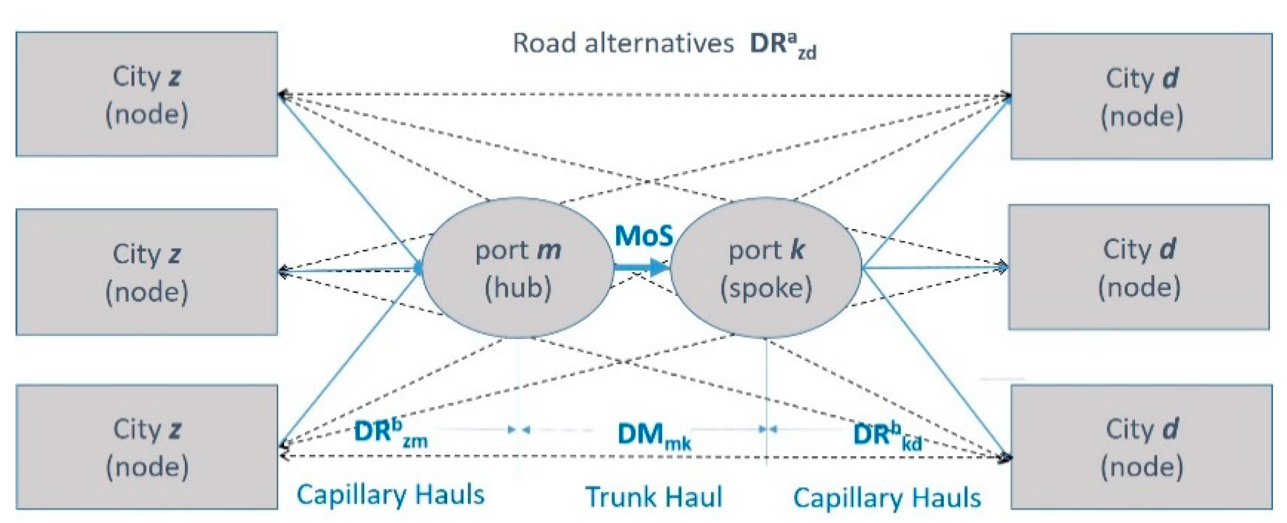
  • Transport networks: A ‘many-to-many’ transport network [18] has been assumed as the transport model in this study (see Figure 1). This means that many possible origins and destinations (nodes) are considered as extreme points of the intermodal chains. This transport model is made up by one trunk haul to transport consolidated cargo (seaborne stretch) and capillary hauls (land hauls). Thus, the capillary hauls refer to land stretches from/to nodes and the ports (consolidation centres for the cargo). Whereas all nodes are extreme points of the chains, regardless of their localization and size, the port category is dependent of its geographical location and its capacity to receive deep sea vessels. Thereby, the ports that receive large vessels from deep sea activity (they are located in the central region of Chile in the application case) are hub ports. The other ports, peripheral ports, are known as spoke ports (see Figure 1).
The ‘many-to-many’ transport network assumed for this study (see Figure 1) uniquely takes two possible nodes in the northern and southern hinterlands (DD = {1, …, d}; see Appendix A) and five nodes in the central region (Z = {1, …, z}; see Appendix A). This decision responds to the geographical location of the main generating centres of loads in Chile regarding the ports.
Thus, the nodes along with the ports (see Figure 1) articulate the capillary hauls of the net. Additionally, the seaborne stretch (trunk haul) is defined by the pair of ports analyzed: hub ports (M = {1, …, m) and spoke ports (K = {1, …, k}; see Appendix A) and they are susceptible to generating MoS. An important assumption has been initially taken; the spoke ports (peripheral ports) move all generated/delivered cargo in the region towards the hub port. Thus, from the hub port, the cargo will be dispatched towards its final destination (nodes): the central or southern regions of Chile or for exportation/importation. Thereby, the hub ports receive cargo from the south towards the north and vice versa; in such a way, they are the common port for the articulation of the northern and southern MoSs and indeed for the connection between the MoS and the long-distance routes for the external traffic (deep sea shipping).
The existence of several possible origins and destinations for the load (nodes) makes it necessary to consider a relative weighting factor for the split of the consolidated cargo among them (see Figure 1). In this case, a probability distribution is assumed in relation to the population of the nodes. Thus, the most populated node will have the highest probability of becoming the final extreme of the load against the rest of the possible nodes in the northern and southern regions (Xd; ∀d ∈ DD; Appendix A). However, the situation is different for the nodes of the central region, because the hub ports by themselves must be considered as nodes as well. This involves assigning to the hub ports a fictitious population able to reflect the external traffic and the cargo from the north with a final destination in the south (instead of the central region) and the opposite, beyond receiving uniquely the load from/to the central region. Consequently, for the nodes in the central region, it will be necessary to consider additional aspects of their probability distribution (Xcjz; ∀z ∈ Z ∧ ∀c ∈ ST ∧ ∀j ∈ J; see Appendix A): the kind of MoS (ST = {c}) and the direction of the transport (J = {1, …, j}).

3.1. Objective Functions

According to the previous explanations, the model introduced is a multi-objective and multi-mode model, and it is formulated through the notation collected in Appendix A. The objective equations reflect the advantage of intermodality with regard to unimodal transport in terms of the costs (F1), time (F2), and environmental impact (F3). These optimization criteria have been selected due to their importance for transport decision makers in terms of service performance [4,8,16,17,19,20,32].
The following equations show the maximization of the unimodality results against intermodality; in other words, a higher value for the objective functions means a greater relative advantage for intermodality.
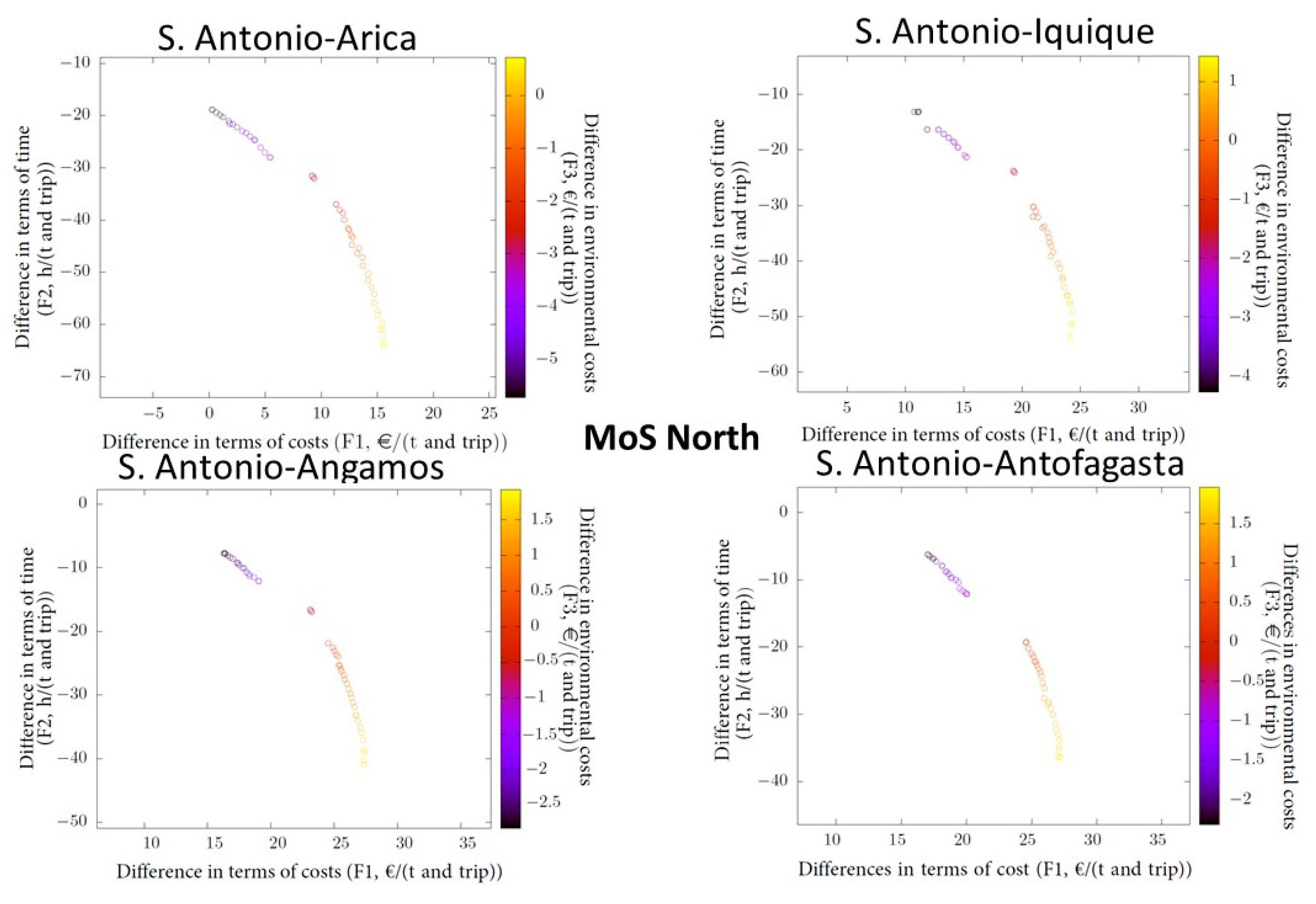
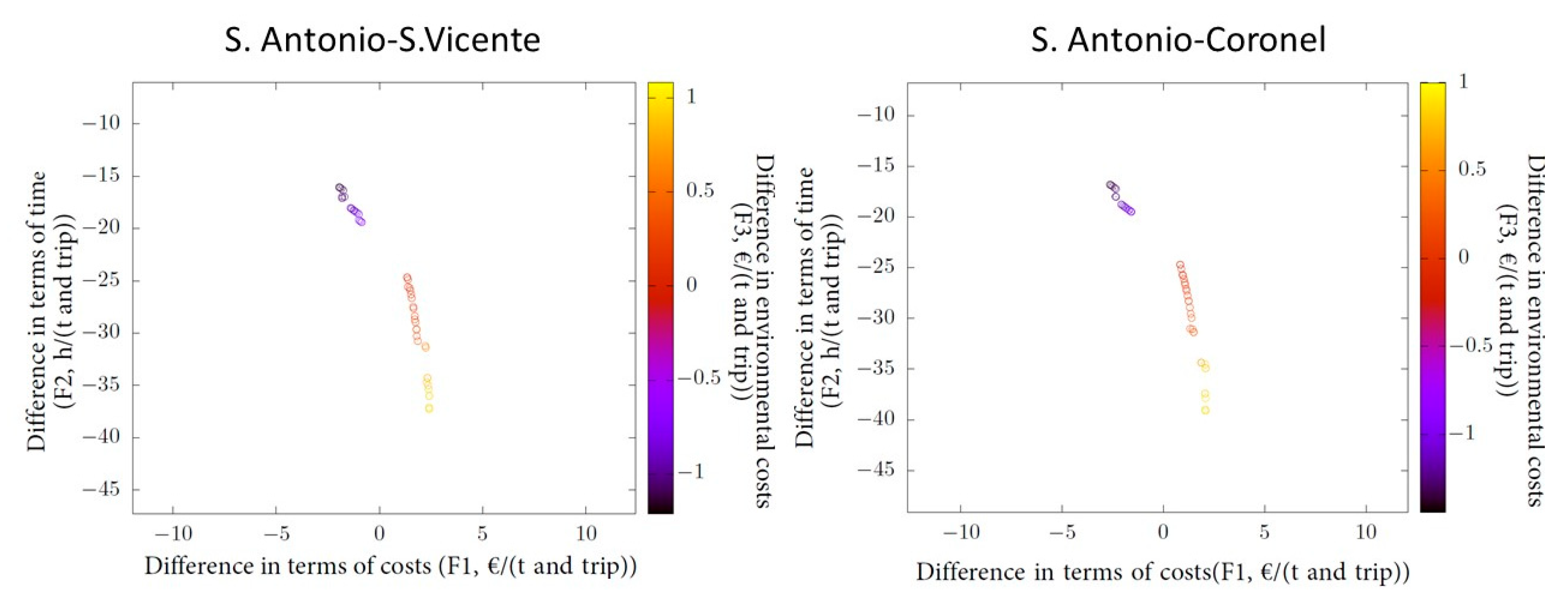
  • Objective 1: The maximization of the relative competitiveness in terms of the overall transport costs (F1) of intermodality (CMU) in relation to unimodality (CU).
F 1 = max ( C U C M U )
C U = R E + ( j = 1 j z = 1 z d = 1 d ( X j z c × X d × D R z d a ) ) × ( 1 2 ) × C K p d P p
C M U = c o s t s c a p i l l a r y _ h a u l s + c o s t s t r u n k _ h a u l
C o s t s c a p i l l a r y _ h a u l s = R E 1 + ( j = 1 j z = 1 z ( X j z c × D R z m b ) ) × ( 1 2 ) × C K p d P p ) + R E 2 + ( d = 1 d ( X d × D R k d b ) ) × C K p d P p
C o s t s t r u n k _ h a u l = R E 3 + 1 ( G p × P p × N t r i p s ) × ( c = 1 12 ( C T c ) )
Equations (1)–(5) (see Table 1 and Appendix A) collect all the costs involved in the transport modes. Thus, beyond the unitary costs of the road transport CKdp (∀p ∈ PP ∧ ∀d ∈ DIS) by considering the weights of the cargo units Pp (p ∈ PP), the probability distributions for the cargo among the nodes (Xd; ∀d ∈ DD and Xcjz; ∀z ∈ Z ∧ ∀c ∈ ST ∧ ∀j ∈ J) and the distances of the legs (DRazd, DRbzm, and DRbkd; see Figure 1), the environmental costs are calculated and integrated into the cost calculations: RE for the trucking and RE1 and RE2 for the capillary hauls. Aside from the environmental impact (RE3), the costs of the trunk hauls are calculated to obtain the minimum required freight. In such a way, twelve cost items are analyzed (CTcc ∈ C; see Appendix A).
  • Objective 2: The maximization of the relative competitiveness in terms of the transit time (F2) of intermodality (TVM) in relation to unimodality (TVU).
Equations (1) and (6) (see Table 1 and Appendix A) show a rising advantage for intermodality with the F2 value. Consequently, the maximization of F2 will be an aim of the model. The Equations (7)–(10) reflect the time invested in road transport for the trucking and capillary hauls.
F 2 = max ( T V U T V M )
T V U = ( 1 / 2 ) × ( j = 1 j z = 1 z d = 1 d ( X j z c × X d × [ D R z d a 16 × V T × 1 + D R z d a V T 16 × 24 + [ ( D R z d a 16 × V T × 1 + D R z d a V T 16 ) D R z d a 16 × V T × 1 + D R z d a V T 16 ] × 16 ] ) )
T V M = t i m e c a p i l l a r y h a u l s + t i m e t r u n k h a u l s
Time c a p i l l a r y _ h a u l s = ( 1 / 2 ) × j = 1 j z = 1 z ( X j z c × [ D R z m b 16 × V T × 1 + D R z m b V T 16 × 24 + [ ( D R z m b 16 × V T × 1 + D R z m b V T 16 ) D R z m b 16 × V T × 1 + D R z m b V T 16 ] × 16 ] ) ) + d = 1 d ( X d × [ D R k d b 16 × V T × 1 + D R k d b V T 16 × 24 + [ ( D R k d b 16 × V T × 1 + D R k d b V T 16 ) D R k d b 16 × V T × 1 + D R k d b V T 16 ] × 16 ] )
T i m e t r u n k _ h a u l = DM mk ( V B × 1.85 ) + w = 1 w TS w + G p NC k × V k + G p NC m × V m
These expressions follow a step structure based on the distances and the configuration of the transport network (see Figure 1 and Appendix A), which responds to the Chilean normative for load driving. This is the maximum permitted speed for a truck (VT) (Art. 145 of Law No. 18.290, Ministry of Transport and Telecommunications of the Government of Chile), 16 h of maximum driving time per day when 2 drivers are demanded (∀d ∈ DIS; see Appendix A), and a minimum resting time of 2 h per driver after 5 driving h (Art. 25 bis of the Code of Work of the Government of Chile). Equation (2) assumes ideal conditions for trucking: continuous transit time and 1 lost hour from changing drivers per driving day. Finally, the time for the seaborne stretch (Equation (10)) integrates the sailing time (this is dependent on the maritime distance, DMmkm ∈ M ∧ ∀k ∈ K and the speed of the vessel, VB), the time related to the port services (pilotage, towing, and mooring service: TSw; ∀w ∈ WW), and the loading and unloading times. For these last elements, the number of cranes for each port (NCk; ∀k ∈ K and NCm; ∀m ∈ M) that simultaneously operate on a vessel and their unitary cycles (Vk, ∀k ∈ K, Vm, ∀m ∈ M) are considered for loading/unloading time of the cargo capacity of the vessel (Gp, ∀p ∈ PP see Appendix A). Additional information about the F1 and F2 equations can be found in the initial models published by Martínez-López et al. (2015 and 2016) [19,20].
  • Objective 3: The maximization of the relative competitiveness in terms of environmental costs (F3) of intermodality (MUE) in relation to unimodality (RE).
Even though the environmental costs (RE, RE1, RE2, and RE3) are added to the objective function (F1), due to their relevant impact on the society, the model analyzes them separately. The pollutants considered are: SO2, NOx, particles PM2.5, and CO2 (U = {1, …, u}). In such a way, the environmental competitiveness of the transport alternatives becomes an aim by itself. The proposed model is a simplification of the method published by Martínez-López et al. (2016) [20] in which all the environmental costs are calculated as a multiplication of the unitary costs (CF1u, CFsuvs ∈ SS ∧ ∀u ∈ U ∧ ∀v ∈ V; see Appendix A) for the pollutants and their emission coefficients (EGsu, EGUu, ∀s ∈ SS ∧ ∀u ∈ U; see Appendix A).
The unitary costs of the pollutants, which are common to both transport alternatives, are taken from the publication by Maibach et al. (2008) [39], and the values are updated to 2015 by applying the CPI index of the country [40,41]. Aside from the population and the emission zone (V = {1, …, v}), these values are dependent on the maritime stage (SS = {1, …, s}). Thus, when free sailing is evaluated, the cost is regardless of the zone (CF1u; ∀u ∈ U). The environmental costs for trucking (unimodal, RE and capillary hauls, RE1 and RE2 in Expressions 12 and 16) follow the method proposed by Ntziabchristos and Samaras (2012) [42], in which the calculation requires, aside from the emission coefficients, the consideration of the fuel consumption of the trucks (FCp, ∀p ∈ PP). For the calculation of the emission coefficients for road transport (EGUuu ∈ U), the Tier 1 method [42] is applied to all pollutants, except for SO2 (Tier 2 method).
F 3 = max ( R E M U E )
R E = u = 1 u j = 1 j z = 1 z d = 1 d ( X j z c × X d × D R z d a × FC p × 10 6 × CF 2 u 2 × EGU u ) 2 × P p
M U E = e n v i r o n m e n t a l _ c o s t s c a p i l l a r y h a u l s + e n v i r o n m e n t a l _ c o s t s t r u n k h a u l s
e n v i r o n m e n t a l c o s t s c a p i l l a r y h a u l s = R E 1 + R E 2
e n v i r o n m e n t a l c o s t s t r u n k h a u l s = R E 3
E n v i r o n m e n t a l _ c o s t s c a p i l l a r y _ h a u l s = u = 1 u j = 1 j z = 1 z ( X jz c × X z × DR z m b × FC p × 10 6 × CF 2 uv × EGU u ) 2 × P p + u = 1 u d = 1 d ( X d × DR k d b × FC p × 10 6 × CF 2 uv × EGU u ) P p
E n v i r o n m e n t a l _ c o s t s t r u n k _ h a u l = 1 ( G p × P p ) × ( u = 1 u ( EG 1 u × DM mk × 0.54 × CF 1 u ) + u = 1 u w = 1 w ( EG 2 u × TS w × CF 2 uv ) + u = 1 u ( EG 3 u × ( G p N C k × V k + G p N C m × V m ) × CF 3 uv ) )
The calculation of the environmental costs for the trunk haul (RE3, Expression 17) is based on the process suggested by Jiang et al. (2014) [40,41], in which the emission coefficients (EGsu; ∀s ∈ SS ∧ ∀u ∈ U) must consider the maritime stages (SS = {1, …, s}) due to their impact on the health of the population. Finally, the emission coefficients for the vessels are calculated through the calculation sheet developed by the Technical University of Denmark (https://www.shipowners.dk/en/services/beregningsvaerktoejer/) in collaboration with the Southern Denmark University [43,44].

3.2. Constraints for the Mathematical Model

Table 2 collects the necessary constraints to provide feasible solutions to the problem analyzed. Constraints RR1 to RR9 ensure the technical feasibility of the vessels.
RR10, RR12, RR13 and RR14 (see Table 2), are highly dependent on the application case; they force the overall cargo capacity of the proposed fleet along with its activity to satisfy the current transport demand for the container load. Finally, RR11 avoids vessels reaching the high-speed craft condition (High Speed Craft Code, MSC 36(63) and Chapter X of Safety of Life at Sea (SOLAS)).

3.3. Resolution of the Model

According to the explanation introduced in the previous paragraphs, the model can be characterized as a multi-objective model with linear and non-linear constraints (see Table 2). Since the Evolutionary Algorithms (EA metaheuristic algorithms) present good results for the resolution of models of this nature [45], the NSGA-II algorithm is used (see Table 3). The parameters shown in Table 1 are the ‘NSGA-II population’s chromosomes’. During the evolution process, the genes take values between −1 and 1. This is required by JEAF, that is, the EA framework used in this work [46].
Using the configuration parameters shown in Table 3, a population of possible solutions have been reached for every iteration. The solutions are evaluated according to the objective functions and the iteration process continues up to meet the maximum number of calls to the evaluation function: 10,000 n (being n the problem dimension; this is the number of optimization variables, see Table 1).

4. Application to Chile

With the widening of the Panama Canal, Chile expects the arrival of bigger vessels with a smaller number of stoppages in the country. Given the necessity to adapt the ports to the larger dimensions of the new vessels, Chile is analyzing the investment in a unique hub port in the central region of the country (the V region). In such a way, the main external traffic of the country moves through this hub port, leaving to the feeder traffic the transport of domestic cargo and the connections among the central region and the rest of the regions in the country. Due to this new reality and the geography of Chile, the articulation of MoS from the V region with the north and the south of Chile seems to be a convenient solution to cope with the transport needs.
In the light of the foregoing, the Chilean case proves to be an interesting challenge for testing the utility of the mathematical model introduced in the previous sections by searching the optimized fleets to maximize the sustainable competitiveness of the intermodality. The analysis will be carried out in three steps:
  • Preliminary scenarios: The competitiveness of the intermodal chains articulated through all possible MoS in the north and in the south will be evaluated using identical conditions (standard values for the port variables). In such a way, the spoke ports with the greatest opportunities for success are identified, by considering uniquely, their geographical localization.
  • Current scenarios: From the previous selection of MoS, a new evaluation of the competitiveness of intermodal chains by operating with optimized fleets is carried out under the current port conditions (real port values). Consequently, the current port performances are included in this second assessment.
  • Sensitivity analysis: The modification of the initial variables will lead to new scenarios. The new frameworks will permit the simulation of the performance and ruggedness of the intermodal chains when the initial scenario changes.

4.1. Data Description

Although the model construction (see Section 3) integrated particular information about the application case (adaptation of the mathematical model), this section shows complementary information to assess Chile’s analysis.
Table 4 collects the information published by the Ministry of Transport and Telecommunications of Chile and Ports [47] about external and domestic trade in tons, that is, general and refrigerated cargo that can be transported by containers. The relevant imbalance between the two directions of the MoS is noteworthy, the direction towards the central region being the most significant in the MoS North and South. This imbalance in the traffic flow, by itself, involves an optimization challenge for the fleets.
Figure 2 shows the extreme nodes (rectangles) of the intermodal chains for the three regions: north, south (DD = {1, …, d} in blue and green), see Appendix A), and central (Z = {1, …, z} in brown). Furthermore, aside from the hub ports (M = {1, …, m}), which are underlined, Figure 2 contains the possible spoke ports for the MoS North and South (K = {1, …, k}, see Appendix A).
On the other hand, once the kind of vehicle has been selected for the road transport (see Section 3), the unitary costs (CKdp, ∀p ∈ PP ∧ ∀d ∈ DIS) are taken from the information published by the Under Secretary of Transport of the Government of Chile [48] (updated to 2015). Furthermore, for the costs related to the seaborne stretch see Equation (1); the following engines are assumed for the optimization of the fleets: a medium-speed and two-tier engine operating with marine diesel oil (MDO) as the fuel type (therefore, any abatement systems are not considered in this analysis). This assumption also influences the value of the emission coefficients EGsu (∀s ∈ SS ∧ ∀u ∈ U) for the trunk haul (see Equation (3)). Finally, owing to the lack of information about the unitary costs for the pollutants in Chile (CFsuv, ∀s ∈ SS ∧ ∀u ∈ U ∧ ∀v ∈ V), the values published for Portugal [39] are taken as a reference, because the calculation models for the unitary costs take into account the population densities, meteorological conditions, and traffic patterns in the countries (distribution of exhaustion emissions), all of these being very closely related to the economic development.

4.2. Preliminary Scenarios

By means of assuming the same port fees and the same port performance (see Appendix B, Table A1), the intermodal chains articulated through different ports will be evaluated under geographic criteria. In such a way, that the analysis uniquely quantifies the performance of the intermodal chains with common extreme points in all cases (DD = {1, …, d} and Z = {1, …, z}; see Appendix A and Figure 2) but with different locations for their cargo consolidation centres (spoke ports (K = {1, …, k}). Furthermore, the assessment considers the ideal conditions for the port operations in all the ports: a direct route for containers in the port [18] and vessels being exempted from pilotage and towing use if they have a bow thruster. Finally, the analysis is carried out for only one hub port (S. Antonio), because the results for the two hub ports will be similar because of their geographical proximity (M = {1, …, m} Valparaíso and S. Antonio, see Figure 2).
Figure 3 and Figure 4 show the results obtained from the simulations of the possible MoS North and South (Pareto fronts). The fleets obtained for the MoS North (see Figure 3) are made up of vessels in the following ranges of cargo capacity, speed and length: 620 ≤ TEUs ≤ 1060, 15 ≤ VB ≤ 25 knots and 117 ≤ L ≤ 140 m. In turn, for the MoS South (see Figure 4), the optimized fleets shown in the Pareto fronts are: 1180 ≤ TEUs ≤ 1500, 15 ≤ VB ≤ 30 knots and 150 ≤ L ≤ 160 m.
The fleet solutions with large and slow vessels (the lower right extreme, see Figure 3 and Figure 4), that prioritize competitiveness in terms of costs (F1), offer better results in terms of the environmental impact (F3); however, they also produce long transit times for the chains (low values for F2). The opposite happens for fleet solutions of quick and small vessels (located at the left upper extreme, see Figure 3 and Figure 4) that maximize the competitiveness in terms of time (F2). The high required power along with a notable reduction of the effects of the economy of scale lead to penalizations in terms of the overall costs (F1) and environmental costs (F3) for the intermodal chains.
The results obtained show negative values for time (F2) in all the cases for the MoS North. This involves penalization for intermodality, which reaches the minimum disadvantage regarding trucking through the S. Antonio–Antofagasta MoS (6 h/t and trip; see Figure 3 and Table 5). Opposite to this, the competitiveness of intermodality through the optimized fleets is positive in terms of the total costs (F1) in all the cases for MoS North (see Figure 3). Again, the highest value for costs (F1) is offered by the S. Antonio–Antofagasta MoS (27€/t and trip; see Figure 3 and Table 5), albeit very close to the results offered by S. Antonio–Angamos. For the MoS North, the intermodality reaches favorable values against the trucking (yellow values in Figure 3) when large and slow vessels are considered, whereas the quick vessel solutions involve an unfavorable impact (black values, see Figure 3). A similar sustainability was found through Angamos and Antofagasta (see Table 5 and Figure 3).
In the MoS South (see Figure 4), the advantage in terms of costs (F1) for intermodality is very reduced and the disadvantage in terms of time (F2) is considerable in all the cases. In addition, the difference in the performance of the intermodal chains through candidate ports in the south (S. Vicente and Coronel) is very slight.
The high dependence on the environmental results (F3), regarding not only the characteristics of the fleets, as stated before (see Figure 3), but also those of the maritime route, is highly remarkable. Thus, whereas the sustainability of intermodality is ensured through Antofagasta (600 nautical miles) when the speed of the vessels is lower than 24 kn, through southern ports (average of 210 nautical miles), the speed of the vessels must be lower than 20 kn.
Table 5 collects fleet solutions with intermediate results in time (F2) and costs (F1) for the MoS North (on the Pareto front) and the maximization of the competitiveness in terms of costs (F1) for the MoS South. According to Table 5, the sustainability of the solutions that is provided by Antofagasta and Angamos ports is similar; however, the intermodality through Antofagasta introduces two advantages regarding Angamos: there is greater competitiveness in terms of time (over five hours) and the necessary fleet needs a lower number of vessels (four versus five). In parallel, the comparison between S. Vicente and Coronel does not prove to be so clear. Even though there is a slight advantage for the intermodal chains through S. Vicente from an environmental standpoint, this is not enough to make a decision for the MoS South.
Due to the very close results obtained through Angamos and Antofagasta in the MoS North and S. Vicente and Coronel in the MoS South, the characteristics of the optimized fleets will be further analyzed in the current scenarios step (the following section) to support the decision-making about spoke ports.

4.3. Current Scenarios

Due to the relevance of the port conditions in the success of the MoS [17] and the intermodal chain, which were selected in the previous section, they will be simulated again but under current conditions. That is, taking the particular values of efficiency and costs of the ports involved (CT7, CT8, CT9, CT10, CT11 and CT12, see Appendix B, Table A1 and Equation (5)).
C M U t r u n k _ h a u l = ( R E 3 + 1 / ( G p × P p × N t r i p s ) × ( c = 1 12 ( C T c ) )
Expression 5 collects the costs of the seaborne stretch in the first objective function (F1; see Equation (1)). Thus, for the current scenario simulations, the port dues-ship dues (CT7), load dues (CT8), mooring dues (CT11), and loading/unloading dues (CT12) are taken from the annexes for the tariffs of 2016 of the Service Handbooks (South Pacific Terminal Valparaíso (TPS), International Terminal Antonio (STI), International Terminal Antofagasta (ATI), and International Terminal of Vicente (SVTI)). The pilotage dues (CT9) are estimated by taking into account the rules of the Chilean Government; firstly, articles 20 and 21 of the Regulation of Pilotage (4th edition, 2015, published by the Directorate General of Maritime Territory and Merchant Shipping) about free maneuvers of pilotage and afterwards, the globalized tariff of Regulation of Tariffs and Rights (2015, article 301, Chapter III), published by the Directorate General of Maritime Territory and Merchant Shipping.
Regarding the towing charges (CT10), the simulations consider the orders published by the harbour master’s office in every port analyzed about the compulsory use of the towing service. In addition, the tariffs offered by the Saam company (https://www.saam.com/en/) are taken for all the cases, due to the fact that the charges from different private companies are very close to each other and are similar for all the ports evaluated.
T V M t r u n k h a u l = w = 1 w TS w + G p NC k × V k + G p NC m × V m
Expression 18 shows the time invested in the trunk haul for the calculation of the second objective function (F2; see Equation (2)). Owing to the lack of information about the time invested in the port operations (TSw, ∀w ∈ WW; see Appendix A), these are assumed from the standard values used for the preliminary scenarios. Appendix B, Table A1 contains the values assumed for the maximum number of cranes able to operate in a vessel for every port (NCkk ∈ K and NCmm ∈ M) and their speeds (Vkk ∈ K and Vmm ∈ M). These data are estimated by taking into account the kinds of cranes and their dimensions according to the information published by the port authorities.
The results obtained from simulations in the current scenarios suggest certain independence of the optimized fleets for the MoS from moderate changes in the port conditions. Proof of this is the proximity of the fleets obtained for the preliminary and current scenarios, and the similar fleets obtained for intermodality through Valparaiso and S. Antonio (both ports are separated by 90.4 km) or through S. Vicente and Coronel (44.2 km apart by road). However, the intermodality results change significantly with the modification of the port conditions (see Table 6). There remains an advantage in costs for intermodality through the MoS North (see Table 6), that could be enough to balance the time penalty regarding trucking for some kinds of non-perishable goods transport. Unlike the MoS North, intermodality through MoS South in the current scenarios is shown to be hardly interesting; an average transit time by road of 6 h for the transport network by truck, whereas the time invested in the intermodal chain reaches 32 h. Only the environmental results (F3) through MoS South could reach favorable values against trucking (see Table 6).
Finally, it is interesting to remark that the simulations in the current scenarios are not conclusive enough to make a clear decision about the most suitable hub port in the V region to articulate the MoSs. The time advantage offered by MoS North through Valparaíso (see Table 6) does not seem to be enough to cope with the higher cost penalization against S. Antonio.

4.4. Sensitivity Analysis

The analysis carried out until now assumed a quantitative evaluation of the intermodal performance by operating with the optimized fleet obtained from the current scenarios (coincident fleet to those obtained to preliminary scenarios, see Table 5). However, this fleet was the optimal one to meet the initial requirements of the transport service (see Table 4) introduced into the model through the constraints RR10, RR12, and RR13 (see Table 2). Despite the unbalanced flow of the demand (see Table 4), the fleet found is able to cope with the total demand estimated in both directions. This involves the fleet offering a greater capacity than the yearly required one, which surpasses 3% through Valparaíso and 5.4% through S. Antonio for the MoS North (Antofagasta). Furthermore, due to the imbalance in the transport flows, the average occupation ratio of the vessels is 74.2% for the MoS North reaching an average ratio of 60.3% in the MoS South for the optimized fleet (see Table 5).
In order to minimize the risk assumed in decisions based on the previous results and to check their robustness, a sensitivity analysis is carried out over the MoS North identified in the previous sections as the most suitable ones (the MoS South will not be analyzed due to their lack of feasibility). Even though many variables are susceptible to be modified, the initial demand is the main driver in the optimization of the fleets; for that reason, it is convenient to determine whether the fleet assumed in this study will offer reasonable results if the initial demand changes. To this aim, a sensitivity analysis is undertaken by modifying in a 20% range over the initial demand (base value, see Table 4) with a positive and negative step of 10% (see Table 7).
Figure 5 shows that the Pareto fronts are almost coincident when the demand changes by keeping the initial imbalance between both senses. This involves the optimal fleet operating under scenarios of analysis that are very close to those obtained from the current scenarios; therefore, the risk assumed with the initial optimized fleet would be low. However, the results of competitiveness if the demand falls would be slightly different (see Table 8).

5. Discussion and Concluding Remarks

This research introduces a mathematical model able to find optimized fleet solutions to operate under MoS conditions by attending to the global competitiveness of the whole chains in relation to trucking. This allows the evaluation of the sustainable performance of ‘door-to-door’ transport through different seaborne alternatives by operating with optimized fleets for them. Consequently, the evaluation capacity of this model surpasses that of the traditional analysis, where the fleets and maritime routes were considered as independent factors. Moreover, since the current model was formulated to attend to different objectives (multi-objective model) at the same time—costs, time, and sustainability in different locations—the results obtained can be analyzed through Pareto fronts and this introduces an effective performance measurement tool for vessel operators, policy makers, heads of ports and other players with decision capacity regarding transport features. This utility is especially significant when taking into account the possibilities of the sensitization of the model.
The heterogeneity of the Chilean transport networks (short and long seaborne legs in the intermodal chains) along with the singularity of their configuration (small shortening of the intermodal distance against the unimodal distance) led to Chile being an effective validation context for the model. This real-life application was attended through three different steps with the intention of resolving three sub-problems: the identification of the MoS between the northern and southern regions with the central regions and their optimized fleets that offer the highest opportunities of success for the intermodality versus the trucking (step 1: preliminary scenarios); the expected performance of the chains under the current conditions of the Chilean ports (step 2: current scenarios); and the influence capacity on the results of modifications on the expected demand and therefore, the risk assumed in decisions about the fleets that were based on the results achieved in the previous steps (step 3: sensitivity analysis).
According to the results, intermodal transport in Chile through the MoS with Antofagasta is the most suitable transport alternative between the northern and the central regions of Chile. By means of operating an optimized fleet for this MoS of 4 container vessels of 580 TEUs at 18 knots of service speed, it would be possible to offer significant advantages in costs (an average of 13 €/t and trip) and environmental savings (an average 0.8 €/t and trip) in relation to trucking. Despite the remarkable time penalty expected for intermodality (an average of 21.5 h regarding the road), this could be offset by the cost saving for non-perishable commodities (user preferences, [49]).
Despite that the model was highly useful to rule out the convenience of establishing an MoS between the southern and the central regions in Chile (this result is not capable of being modified by any actor), it was not able to provide enough elements to determine the most suitable hub port in the central region of the country (Valparaíso or S. Antonio) for the articulation of the MoS. Since both ports are closely similar (Port Performance Indicators) and neighbors (small distance between them), the exploring cooperation strategies between them and the shipping companies in medium term could facilitate the decision about the port expansion in Chile [50].
Aside from the results achieved for Chile, this application case has allowed us to test the model utility. Additionally, the sensitivity analysis carried out on this case has provided general findings about intermodal performance; whereas moderate modifications of the port conditions do not alter the suitability of fleets optimized for MoS under initial conditions, these modifications can have a relevant impact on the performance of the whole chain. This finding is in line with the conclusions of previous works that have focused on different geographical regions [17]. However, moderate modifications on the initial demand have not compromised the adequacy of the initial fleets to the routes or the expected competitiveness results. Further research lines on this model are expected through the implementation of additional objective functions. In this way, more detailed information will be able to reach a wider group of stakeholders (synchromodality).

Author Contributions

Data curation, M.C.; Formal analysis, A.M.-L.; Methodology, A.M.-L.; Resources, M.C.; Validation, A.M.-L.; Writing—original draft, M.C. All authors have read and agreed to the published version of the manuscript.

Funding

This research received no external funding.

Acknowledgments

Many thanks to the anonymous reviewers for their time dedicated to improving this paper.

Conflicts of Interest

The authors declare no conflict of interest.

Appendix A

Subscripts:
A = {1, …, a}Different legs for the intermodal chains: capillary hauls (road haulage in both costs) and the trunk haul (maritime route).
BB = {1, …, b}Installation of bow thruster: no or yes.
C = {1, …, c}Cost inputs to reach the minimum required freight: amortization costs, financing costs, insurance costs, maintenance costs, crew costs, fuel costs, and port tariff costs (ship dues, cargo dues, pilot tariff, towing tariff, mooring dues, and loading/unloading costs).
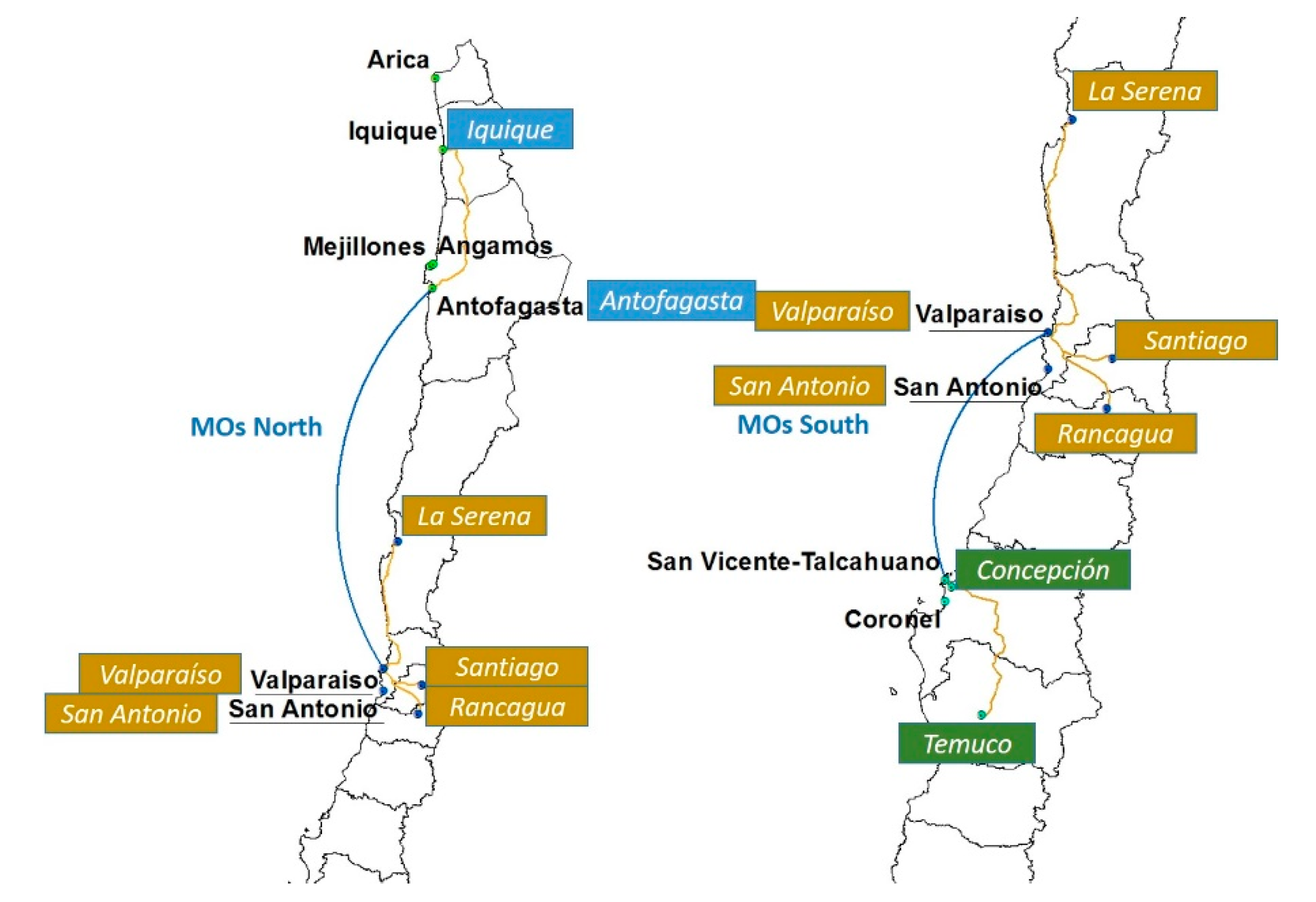
DD = {1, …, d}Final destinations on land (nodes). For the transport network of the application case, Iquique and Antofagasta are used in the northern region and Concepción and Temuco are used in the southern region.
EE = {1, …, e}Kind of main engines: diesel engines and turbines.
GG = {1, …, g}Cargo-handling systems: vessel cranes or port cranes.
H = {1, …, h}Possible propellers: screws or waterjets.
I = {1, …, i}Number of main engines.
J = {1, …, j}Direction for the transport (north–south and south–north).
K = {1, …, k}Possible spoke ports. For the application case, they are Arica, Iquique, Mejillones, and Antofagasta in the northern region and San Vicente and Coronel in the southern region.
M = {1, …, m}Possible hub ports. For the application case, they are Valparaíso and San Antonio in the V region.
N = {1, …, n}Number of shaft lines in the machine room.
PP = {1, …, p}Types of cargo units for container vessels: TEUs and FEUs.
SS = {1, …, s}Stages during maritime transport: free sailing, maneuvering (pilotage time, towing time, and mooring time), and berthing (loading and unloading operations).
U = {1, …, u}Group of evaluated pollutants: SO2, NOx, PM2.5, and CO2.
V = {1, …, v}Classification of the zones according to the harmful impact of the emissions: metropolitan zone and urban zone.
WW = {1, …, w}Port services for the maneuvering stage: pilotage, towing, and mooring services.
Z = {1, …, z}The origins on land (nodes). For the transport network of the application case, in the central region, are Santiago, Valparaíso hub port (Valparaíso or San Antonio), La Serena, and Rancagua are used.
Superscripts:
ST = {c}The MoS analyzed: MoS North and MoS South.
DIS = {d}Compulsory driving with two drivers (no and yes).
Variables:
BBreadth of the vessels (m).
CTcCost of the items for the maritime required freight of the trunk haul (€); ∀c ∈ C
CMUOverall transport costs for the intermodal chain (€/(t×trip)).
CUOverall transport costs for the unimodal alternative (€/(t×trip)).
DDepth to the upper deck (m).
EGsuEmission coefficients for container vessels during the different maritime stages (kg/nm and in kg/h); ∀s ∈ SS ∧ ∀u ∈ U.
EGUuEmission coefficients for trucking (gr of pollutant/kg of fuel consumed); ∀u ∈ U.
FBFreeboard (m).
FCpFuel consumption for trucks by considering the cargo unit transported (gr fuel/km); ∀p ∈ PP.
GpCargo units related to the cargo capacity of the vessel; ∀p ∈ PP.
GTGross Tonnage.
Llength of the vessels (m).
MGgCargo handling systems ∀g ∈ GG.
MMbBow thruster installation ∀b ∈ BB.
MUEEnvironmental costs for the intermodal chains (€/(t×trip)).
NBNumber of vessels.
NCkNumber of cranes per vessel ∀k ∈ K.
NCmNumber of cranes per vessel ∀m ∈ M.
NtripsAnnual trips for the fleet.
NMEiNumber of main engines for the vessels ∀i ∈ I.
NSLnNumber of shaft lines in the vessels; ∀n ∈ N.
REEnvironmental costs (€/(t×trip)) for the road transport.
REaEnvironmental costs (€/(t×trip)) for the stretches of the intermodal chain ∀a ∈ A.
TSummer draught (m).
PBPropulsion Power for the vessels (HP).
TMEeType of Main Engines; ∀e ∈ EE.
TPhType of propeller; ∀h ∈ H.
TPMDeadweight (t).
TSwTime for every port operation during the maneuvering stage (h); ∀w ∈ WW.
TVMTime invested in the intermodal transport (h).
TVUTime invested in the unimodal alternative (road haulage) (h).
VBSpeed of the vessel (knots).
VTSpeed of the truck (km/h).
Buoyancy volume (m3).
Inputs:
CF1uUnitary costs for the pollutants during free sailing (€/kg); ∀u ∈ U.
CFsuvUnitary costs for the pollutants considering the maritime stages and the affected zones (€/kg); ∀s ∈ SS ∧ ∀u ∈ U ∧ ∀v ∈ V.
CKdpUnitary cost per kilometer by road (unimodal; the value is dependent on the required number of drivers and the cargo unit transported (€/km)); ∀p ∈ PP ∧ ∀d ∈ DIS.
DMmkMaritime distance for the trunk haul (km); ∀m ∈ M ∧ ∀k ∈ K.
DRazdRoad distance for the unimodal alternative (km); ∀z ∈ Z ∧ ∀d ∈ DD.
DRbzmRoad distance for the capillary hauls in the intermodal chains from/to hub ports (km); ∀z ∈ Z ∧ ∀m ∈ M.
DRbkdRoad distance for the capillary hauls in the intermodal chains from/to spoke ports (km); ∀k ∈ K ∧ ∀d ∈ DD.
XdRelative probability of delivering/receiving a load for each node of the northern and southern regions (%) regarding other alternative nodes ∀d ∈ DD.
XcjzRelative probability of delivering/receiving a load for each node of the central region (%) regarding other alternative nodes for each MoS (MoS North and MoS South) and direction (north–south and south–north) ∀z ∈ Z ∧ ∀c ∈ ST ∧ ∀j ∈ J.
Ppweights for the cargo units (tons); (p ∈ PP)
VkAverage speed of the cranes for the spoke ports ∀k ∈ K (cycles/h).
VmAverage speed of the cranes for the hub ports ∀m ∈ M (cycles/h).

Appendix B

Table A1. Unitary port costs for the preliminary and current scenarios (2015).
Preliminary ScenariosCurrent Scenarios
For Every PortValparaísoS. AntonioAntofagastaS. VicenteCoronel
Maximum Number of cranes/vessels (NCk and NCm) unitsno limit66374
Average speed/crane (Vk and Vm) (cycle/h)272727181822.5
Ship dues (CT7) (€/GT h)0.01671.5361.5741.9542.6182.772
Cargo dues (CT8) (€/TEU)32.737.958.363.8633.8634.08
(€/FEU)49.10413.0413.61104.7255.5355.9
Pilot dues (CT9)(GT < 10,000)(€)231.28112.68112.68112.68112.68112.68
(GT ≥ 10,000)(€)460.6337.71337.71000
Towing dues (CT10)(GT < 13,000)(€/tug)420.12995.35995.35995.35995.35995.35
(GT ≥ 13,000)(€/tug)1093.422190.692190.692190.692190.692190.69
Mooring dues (CT11)(GT < 3000)(€/mooring)96.350000390.87
(GT ≥ 3000)(€/mooring)316.150000390.87
Loading/unloading dues (CT12) (€/TEU)24.8183.3573.0582.5463.6372.72
(€/FEU)49.61124.98109.56128.998.1690.90

References

  1. Brooks, M.R.; Frost, J.D. Short Sea Shipping: A Canadian Perspective. Marit. Policy Manag. 2004, 31, 393–407. [Google Scholar] [CrossRef]
  2. Brooks, M.R.; Sanchez, R.J.; Wilmsmeier, G. Developing Short Sea Shipping in South America—Looking Beyond Traditional Perspectives. Ocean Yearb. Online 2014, 28, 495–526. [Google Scholar] [CrossRef] [Green Version]
  3. Brooks, M.; Wilmsmeier, G. A Chilean Maritime Highway: Is It a Possible Domestic Transport Option? Transp. Res. Rec. 2017, 2611, 32–40. [Google Scholar] [CrossRef]
  4. Puckett, S.; Hensher, D.; Brooks, M.; Trifts, V. Preferences for alternative short sea shipping opportunities. Transp. Res. Part E Log. Transp. Rev. 2011, 47, 182–189. [Google Scholar] [CrossRef]
  5. Bendall, H.; Brooks, M. Short sea shipping: Lessons for or from Australia. Int. J. Shipp. Transp. Logist. 2011, 3, 2011. [Google Scholar] [CrossRef]
  6. Chang, Y.; Lee, P.; Kim, H. Optimization Model for Transportation of Container Cargoes considering Short Sea Shipping and External Cost. South Korean Case. Transp. Res. Rec. 2010, 2166, 99–108. [Google Scholar] [CrossRef]
  7. Lee, P.; Hu, K.C.H.; Chen, T. External Costs of Domestic Container Transportation: Short-Sea Shipping versus Trucking in Taiwan. Transp. Rev. 2010, 30, 315–335. [Google Scholar] [CrossRef]
  8. Suárez-Alemán, A.; Trujillo, L.; Medda, F. Short sea shipping as intermodal competitor: A theoretical analysis of European transport policies. Marit. Policy Manag. 2015, 42, 317–334. [Google Scholar] [CrossRef]
  9. Takano, K.; Arai, M. A genetic algorithm for the hub-and-spoke problem applied to containerized cargo transport. J. Mar. Sci. Technol. 2009, 14, 256–274. [Google Scholar] [CrossRef]
  10. Hjelle, M.H. Short sea shipping’s green label at risk. Transp. Rev. 2010, 30, 617–640. [Google Scholar] [CrossRef]
  11. Hjelle, M.H. Atmospheric emissions of short sea shipping compared to road transport though the peaks and troughs of short-term market cycles. Transp. Rev. 2014, 34, 379–395. [Google Scholar] [CrossRef]
  12. Hjelle, M.H.; Fridell, E. When is short sea shipping environmentally competitive? In Environmental Health—Emerging Issues and Practice; Oosthuizen, J., Ed.; InTech: Rijeka, Croatia, 2012. [Google Scholar]
  13. Culliane, K.; Culliane, S. Atmospheric emissions from shipping: The need for regulation and approaches to compliance. Transp. Rev. 2013, 33, 377–401. [Google Scholar] [CrossRef]
  14. Bengtsson, S.; Fridell, E.; Andersson, K. Fuels for short sea shipping: Comparative assessment with focus on environment impact. Proc. Inst. Mech. Eng. M 2014, 228, 44–54. [Google Scholar] [CrossRef]
  15. Xie, X.; Xu, D.L.; Yang, J.B.; Wang, J.; Ren, J.; Yu, S. Ship selection using a multiple-criteria synthesis approach. J. Mar. Sci. Technol. 2008, 13, 50–62. [Google Scholar] [CrossRef]
  16. Giusti, R.; Iorfida Ch Li, Y.; Manerba, D.; Musso, S.; Perboli, G.; Tadei, R.; Yuan, S. Sustainable and De-Stressed International Supply-Chains Through the SYNCHRO-NET Approach. Sustainability 2019, 11, 1083. [Google Scholar] [CrossRef] [Green Version]
  17. Žgaljić, D.; Tijan, E.; Jugović, A.; Jugović, T.P. Implementation of Sustainable Motorways of the Sea Services Multi-Criteria Analysis of a Croatian Port System. Sustainability 2019, 11, 6827. [Google Scholar] [CrossRef] [Green Version]
  18. Daganzo, C. Many to many distribution. In Logistic Systems Analysis; Daganzo, C., Ed.; Springer: Berlin, Germany, 2005. [Google Scholar]
  19. Martínez-López, A.; Caamaño, P.; Castro, L. Definition of optimal fleets for Sea Motorways: The case of France and Spain on the Atlantic coast. Int. J. Shipp. Transp. Logist. 2015, 7, 89–113. [Google Scholar] [CrossRef]
  20. Martínez-López, A.; Caamaño, P.; Míguez, M. Influence of external costs on the optimisation of container fleets by operating under motorways of the sea conditions. Int. J. Shipp. Transp. Logist. 2016, 8, 653–686. [Google Scholar] [CrossRef]
  21. Yan, S.; Chen, C.Y.; Lin, S.C. Ship scheduling and container shipment planning for liners in short-term operations. J. Mar. Sci. Technol. 2009, 14, 417–435. [Google Scholar] [CrossRef]
  22. Fan, H.; Yu, J.; Liu, X. Tramp Ship Routing and Scheduling with Speed Optimization Considering Carbon Emissions. Sustainability 2019, 11, 6367. [Google Scholar] [CrossRef] [Green Version]
  23. Wang, S.; Meng, Q. Sailing speed optimization for container ships in a liner shipping network. Transp. Res. E Log. Transp. Rev. 2012, 48, 701–714. [Google Scholar] [CrossRef]
  24. Kim, J.-G.; Kim, H.-J.; Lee, P.T.-W. Optimising containership speed and fleet size under a carbon tax and an emission trading scheme. Int. J. Shipp. Transp. Logist. 2013, 5, 571–590. [Google Scholar] [CrossRef]
  25. Chandra, S.; Christiansen, M.; Fagerholt, K. Combined fleet deployment and inventory management in roll-on/roll-off shipping. Transp. Res. E Log. Transp. Rev. 2016, 92, 43–55. [Google Scholar] [CrossRef]
  26. Karsten, C.V.; Ropke, S.; Pisinger, D. Simultaneous Optimization of Container Ship Sailing Speed and Container Routing with Transit Time Restrictions. Transp. Sci. 2018, 52, 769–787. [Google Scholar] [CrossRef] [Green Version]
  27. Mansouri, S.A.; Lee, H.; Aluko, O. Multi-objective decision supports to enhance environmental sustainability in maritime shipping: A review and future directions. Transp. Res. Part E Log. Transp. Rev. 2015, 78, 3–18. [Google Scholar] [CrossRef]
  28. Wong, E.Y.; Yeung, H.S.; Lau, H.Y. Immunity-based hybrid evolutionary algorithm for multi-objective optimization in global container repositioning. Eng. Appl. Artif. Intel. 2009, 22, 842–854. [Google Scholar] [CrossRef]
  29. Wong, E.Y.C.; Lau, H.Y.; Mak, K.L. Immunity-based evolutionary algorithm for optimal global container repositioning in liner shipping. Or Spectrum 2010, 32, 739–763. [Google Scholar] [CrossRef] [Green Version]
  30. Chen, G.; Govindan, K.; Golias, M.M. Reducing truck emissions at container terminals in a low carbon economy: Proposal of a queueing-based Biobjective model for optimizing truck arrival pattern. Transp. Res. Part E Log. Transp. Rev. 2013, 55, 3–22. [Google Scholar] [CrossRef]
  31. Hu, Q.; Hu, Z.; Du, Y. Berth and quay-crane allocation problem considering fuel consumption and emissions from vessels. Comput. Ind. Eng. 2014, 70, 1–10. [Google Scholar] [CrossRef]
  32. Baykasoglu, A.; Subulan, K. A multi-objective sustainable load planning model for intermodal transportation networks with a real-life application. Transp. Res. Part E Log. Transp. Rev. 2016, 95, 207–247. [Google Scholar] [CrossRef]
  33. Martínez-López, A.; Caamaño, P.; Chica, M.; Trujillo, L. Optimization of a container vessel fleet and its propulsion plant to articulate sustainable intermodal chains versus road transport. Transp. Res. Part D Transp. Environ. 2018, 59, 134–147. [Google Scholar] [CrossRef]
  34. Ministry of Transportation of Chile. 2014. Available online: http://www.sepchile.cl/documentacion/estadisticas-portuarias/?no_cache=1 (accessed on 12 February 2020).
  35. Usabiaga, J.; Castells, M.; Martínez, X.; Olcer, A. A simulation model for road and maritime environmental performance assessment. J. Environ. Prot. Ecol. 2013, 4, 683–693. [Google Scholar] [CrossRef] [Green Version]
  36. Lupi, M.; Farina, A.; Orsi, D.; Pratelli, A. The capability of Motorways of the Sea of being competitive against road transport. The case of the Italian mainland and Sicily. J. Transp. Geogr. 2017, 58, 9–21. [Google Scholar] [CrossRef] [Green Version]
  37. Under Secretary of Transport, Ministry of Transport and Telecommunications of the Government of Chile. Analysis of the Transport. of National Cargo. 2009. Available online: http://www.subtrans.cl/subtrans/doc/Informefinalcorregido.pdf (accessed on 12 February 2020).
  38. National Institute of Statistics of Chile. Yearbook about the Road Transport. 2013. Available online: http://www.ine.cl/canales/chile_estadistico/estadisticas_economicas/transporte_y_comunicaciones/encuesta-estructural-transporte-carretera/2013/infografia_transporte_por_carretera_2015.pdf (accessed on 12 February 2020).
  39. Maibach, M.; Schreyer, C.; Sutter, D.; Essen, H.P.V.; Boon, B.H.; Smokers, R.; Schrote, A.; Doll, C.; Pawlowska, B.; Bak, M. Handbook on Estimation of External Costs in the Transport Sector; CE Delft: Delft, The Netherlands, 2008. [Google Scholar]
  40. Jiang, L.; Kronbak, J. The Model of Maritime External Costs; Project No. 2010-56, Emissionsbeslutingsstottesystem, Word Package 1, Report No. 06; University of Southern Denmark: Odense, Denmark, 2012. [Google Scholar]
  41. Jiang, L.; Kronbak, J.; Christensen, L. The cost and benefits of sulphur reduction measures:Sulphur scrubbers versus marine gas oil. Transp. Res. Part D Transp. Environ. 2014, 28, 19–27. [Google Scholar] [CrossRef]
  42. Ntziabchristos and Samaras. Passenger cars, light duty trucks, heavy duty vehicles including buses and motorbikes. In EMEP/EEA Air Pollutant Emission Inventory Guidebook 2009 (updated May, 2012); Technical Report No. 9/2009; The European Environment Agency: Copenhagen, Denmark, 2012. [Google Scholar]
  43. Kristensen, H. Energy Demand and Exhaust Gas Emissions of Ships; Work Package 2 of Project Emissionsbeslutningsstottesystem; Technical University of Denmark: Copenhagen, Denmark, 2012. [Google Scholar]
  44. Lützen, M.; Kristensen, H. A model for prediction of propulsion power and emissions tankers and bulk carriers. In Proceedings of the World Maritime Technology Conference, Saint Petersburg, Russia, 29 May–1 June 2012. [Google Scholar]
  45. Possel, B.; Wismans, L.; Van Berkum, E.; Bliemer, M. The multi-objective network design problem using minimizing externalities as objectives: Comparison of a genetic algorithm and simulated annealing framework. Transportation 2018, 45, 545–572. [Google Scholar] [CrossRef]
  46. Caamano, P.; Tedin, R.; Paz-Lopez, A.; Becerra, J.A. JEAF: A Java evolutionary algorithm framework. In Proceedings of the 2010 IEEE Congress on Evolutionary Computation (CEC), Barcelona, Spain, 18–23 July 2010; pp. 1–8. [Google Scholar]
  47. Directemar. Ministry of Transport and Telecommunications of Chile and Ports. 2012. Available online: http://web.directemar.cl/estadisticas/puertos/default.htm (accessed on 12 February 2020).
  48. Under Secretary of Transport; Ministry of Transport and Telecommunications of the Government of Chile. Analysis of the Costs and Competitiveness of the Modes of Interurban Land Transport. 2011. Available online: http://www.subtrans.cl/subtrans/doc/Informefinalcorregido.pdf (accessed on 12 February 2020).
  49. Reis, V. Analysis of mode choice variables in short-distance intermodal freight transport using an agent-based model. Transp. Res. Part A Policy Pract. 2014, 61, 100–120. [Google Scholar] [CrossRef]
  50. Asgari, N.; Zanjirani Farahani, R.; Goh, M. Network design approach for hub ports-shipping companies competition and cooperation. Transp. Res. Part A Policy Pract. 2013, 48, 1–18. [Google Scholar] [CrossRef]
Figure 1. ‘Many to Many’ transport network.
Sustainability 12 02221 g001
Figure 2. Extreme nodes and possible hub and spoke ports for the MoS.
Sustainability 12 02221 g002
Figure 3. Pareto fronts for intermodal chains articulated through different spoke ports for the MoS North.
Sustainability 12 02221 g003
Figure 4. Pareto fronts for intermodal chains articulated through different spoke ports for the MoS South.
Sustainability 12 02221 g004
Figure 5. Pareto fronts for intermodal chains articulated through MoS North when the demand is modified.
Sustainability 12 02221 g005
Table 1. Main characterization variables of the fleet.
VBSpeed of the vessel (kn)
Gp: ∀p ∈ PPCargo Capacity for the vessels (units)
MGg; ∀g ∈ GGCargo handling systems
MMb; ∀b ∈ BBBow thruster installation
NtripsAnnual trips for the fleet
NBNumber of vessels
LLength between perpendiculars (m)
BBreadth (m)
DDepth to the upper deck (m)
TSummer draught (m)
FBFreeboard (m)
GTGross tonnage (t)
Buoyancy volume (m3)
TPMDeadweight (t)
PBPropulsion Power (HP)
TMEe; ∀e ∈ EEType of Main Engines
TPh; ∀h ∈ HType of propeller
NSLn; ∀n ∈ NNumber of shaft lines
NMEi; ∀i ∈ INumber of main engines
(See Appendix A for subscripts).
Table 2. Constraints for the mathematical model.
RR1 T < 10
RR2 F B > F B m i n i m u m
RR3 G p ( f i n a l ) G p   ( e s t i m a t e d )
RR4B ≥ 13.56
RR5D7.15 if PB ≤ 33,794
5 × 10 4 × P B 5.52  if 33,794 < PB ≤ 53,600
RR6 4.94 < L / B < 7.50
RR7 1.55 < B / D < 2.31
RR8 7.85 < L / D < 14.17
RR9 2.35 < B / T < 3.20
RR10 672 N t r i p s 384
RR11 V B < ( 3.7 × 0 , 1667 / 0.514 )
RR12Gp × NtripsMoS (North)370,566;  if Gp = G1
225,955;  if Gp = G2
MoS (South)791,408;  if Gp = G1
482,566;  if Gp = G2
RR13(Gp/2) × NtripsMoS (North)276,973;  if Gp = G1
168,886;  if Gp = G2
MoS (South)709,542;  if Gp = G1
432,648;  if Gp = G2
RR14 T V B N B × 12
Table 3. Configuration parameters for NSGA-II.
OperatorParametersValues
Tournament SelectionPool Size2
SBX-CrossoverProbability5%
Polynomial MutationProbability60%
N1
Table 4. Yearly transport needs for MoS per direction.
Ports of NorthNorth–South & CentreSouth & Centre–North
Region(Exports and Cabotage) (t)(Imports and Cabotage) (t)
Arica124,835147,394
Iquique412,94875,311
Mejillones122,186121,964
Angamos1,576,985570,598
Antofagasta1,225,215254,636
North Total3,462,1681,169,903
Ports of SouthNorth & Centre–SouthSouth–North & Centre
Region(Imports and Cabotage) (t)(Exports and Cabotage) (t)
Lirquen62,5763,144,777
San Vicente657,9113,612,814
Coronel302,8322,111,696
South Total1,023,3198,869,287
Source: Directemar, 2012.
Table 5. Solutions of optimized fleets for the MoS in the preliminary scenarios though S. Antonio.
FleetsAngamosAntofagastaS. VicenteCoronel
Cargo unitsFEUsFEUsFEUsFEUs
Cargo capacity (Gp)761 TEUs608 TEUs1334 TEUs1330 TEUs
Speed of the vessels (kn)17.2616.9016.1116.58
Bow thrusterYes (MM2)Yes (MM2)Yes (MM2)Yes (MM2)
Cargo handling systemsPort cranes (MG2)Port cranes (MG2)Port cranes (MG2)Port cranes (MG2)
Number of vessels (NB)5433
Yearly trips (N)668670672672
L (m)127.56118.49158.2157.8
B (m)21.4520.1527.4127.34
D (m)10.559.8513.3213.27
GT (Ton)8.2316.79816.61216.268
PropellerConventional Screw (TP1)Conventional Screw (TP1)Conventional Screw (TP1)Conventional Screw (TP1)
Number of shaft lines1 (NSL1)1 (NSL1)1 (NSL1)1 (NSL1)
Main engineDiesel (TME1)Diesel (TME1)Diesel (TME1)Diesel (TME1)
Number of main engines1 (NME1)1 (NME1)1 (NME1)1 (NME1)
RESULTS
F1(€/(t×trip))25.8025.411.851.50
F2(h/(t×trip))−27.58−22.73−30.75−31.36
F3(€/(t×trip)1.021.040.460.37
Table 6. Range of results for the simulations of the MoS operating with optimized fleets in both scenarios.
Spoke PortsObjective FunctionsPreliminary ScenariosCurrent Scenarios
S. AntonioS. AntonioValparaíso
AntofagastaF1 (€/t and trip)[17; 27][6.14.; 16.1][5.9.; 15.5]
F2 (h/t and trip)[−36; −6][−44; −9.1][−38; −8]
F3 (€/t and trip)[−2; 2][−2; 2][−2; 2]
S. VicenteF1 (€/t and trip)[−1.9; 2.4][−7.24; −3.1][−6.6; −2.0]
F2 (h/t and trip)[−36; −16][−37.2; −16.0][−37.8; −16]
F3 (€/t and trip)[−1.1; 0.9][−1.1; 1.1][−1.2; 1.1]
CoronelF1 (€/t and trip)[−2.6; 2.1][−8; −3.7][−7.5; −2,6]
F2 (h/t and trip)[−34.9; −16.8][−41.7; −18.2][−42.6; −18.1]
F3 (€/t and trip)[−1.3; 0.8][−1.3; 0.9][−1.5; 1,0]
Table 7. Assessment scenarios for the sensitivity analysis.
Scenario 1Scenario 2Scenario 3 = Current ScenarioScenario 4Scenario 5
120%110%100%90%80%
Base ValueBase ValueBase ValueBase ValueBase Value
Table 8. Sensitivity results of the intermodal chains through MoS North when the initial demand falls.
Demand
AntofagastaF1(€/t Trip)F2 (h/t Trip)F3 (€/t Trip)
ValparaísoScenario 3 (100%) = Base Value12.92−21.000.87
Scenario 4 (90%)12.80−20.690.85
Scenario 5 (80%)12.56−20.550.85
S. AntonioScenario 3 (100%) = Base Value13.26−22.170.71
Scenario 4 (90%)13.05−22.140.72
Scenario 5 (80%)13.10−22.010.71

