Optimizing the Environmental and Economic Sustainability of Remote Community Infrastructure

Abstract

Remote communities such as rural villages, post-disaster housing camps, and military forward operating bases are often located in remote and hostile areas with limited or no access to established infrastructure grids. Operating these communities with conventional assets requires constant resupply, which yields a significant logistical burden, creates negative environmental impacts, and increases costs. For example, a 2000-member isolated village in northern Canada relying on diesel generators required 8.6 million USD of fuel per year and emitted 8500 tons of carbon dioxide. Remote community planners can mitigate these negative impacts by selecting sustainable technologies that minimize resource consumption and emissions. However, the alternatives often come at a higher procurement cost and mobilization requirement. To assist planners with this challenging task, this paper presents the development of a novel infrastructure sustainability assessment model capable of generating optimal tradeoffs between minimizing environmental impacts and minimizing life-cycle costs over the community’s anticipated lifespan. Model performance was evaluated using a case study of a hypothetical 500-person remote military base with 864 feasible infrastructure portfolios and 48 procedural portfolios. The case study results demonstrated the model’s novel capability to assist planners in identifying optimal combinations of infrastructure alternatives that minimize negative sustainability impacts, leading to remote communities that are more self-sufficient with reduced emissions and costs.

1. Introduction

Remote communities such as rural villages, post-disaster housing camps, and military forward operating bases (FOB) are often detached from established infrastructure grids and require a constant resupply of resources. This resource dependence presents sustainability challenges such as a significant logistical burden, negative environmental impacts, and increased costs [1,2]. In one example, a 2000-member isolated village in northern Canada relying solely on diesel generators required 2.95 million liters of fuel per year to support its power requirement [3]. The fuel cost $8.6M USD and emitted 8500 tons of CO₂—the annual equivalent of nearly 1700 passenger vehicles.

For the purposes of this research effort, sustainability refers to the planning and implementation of conservation measures and infrastructure alternatives that reduce reliance on fossil fuels, conserve water, minimize waste streams, abate negative environmental impacts, and promote self-sufficient operations [4]. While this definition addresses only one portion of a broader sustainability challenge at remote communities, it enables the quantification and mitigation of negative environmental impacts and costs resulting directly from infrastructure decisions. Planners may choose to enhance the proposed objective function by adding measures of sustainability or adapting the function to be more reflective of the community in question. In the present application, power production, water production, and waste management systems are of primary concern, due to their direct impact on sustainability objectives and logistical requirements for resources such as fuel, water, and waste [5,6]. Remote community planners have the opportunity to select technologies that will reduce the negative sustainability impacts [7], but such alternatives are often bulky to transport and expensive to procure [8]. Both the environmental impact and the cost involved with mobilizing equipment-based components can negatively impact sustainability objectives based on the item’s size, weight, and mode of delivery. Accordingly, planners are faced with the challenging task of selecting infrastructure alternatives that optimize initial and operational tradeoffs between environmental and economic performance.

A number of studies have been conducted that (1) quantify the environmental impact of infrastructure; (2) identify tradeoffs between the environmental and economic impact of infrastructure alternatives; and (3) optimize tradeoffs between sustainability objectives for remote communities. First, various research efforts have quantified the environmental sustainability of infrastructure, including power production methods [9,10,11]; water production methods [12,13]; wastewater management systems [14,15]; and solid-waste management systems [16,17,18]. These efforts quantified environmental sustainability through various indicators, such as greenhouse gas (GHG) emissions, pollution emissions, energy consumption, embodied emissions, and global warming potential. These indicators can be quantified at a static point in time, such as embedded emissions of materials, or over the infrastructure’s lifetime via a life-cycle assessment.

Second, additional studies identified tradeoffs between the environmental and economic sustainability of infrastructure alternatives. For example, Karatas and El-Rayes [19] utilized GHG emissions, water consumption, and initial cost metrics to assess the integration of green building measures and fixtures into housing units, generating optimal tradeoffs between environmental impact and cost. Alternatively, Ozcan-Deniz et al. [20] utilized a global warming potential metric to optimize the selection of construction activities, thereby minimizing project time, cost, and environmental impact. Additional economic metrics include energy consumption, transportation requirements, operating costs, and life-cycle costs [21].

Third, other research efforts optimized tradeoffs between sustainability objectives for remote communities. Optimization is the process by which one determines the best solution to a problem based on a set of constraints [22]. When this process includes just one objective, the intent is to determine one ideal solution. A multi-objective optimization problem, however, occurs when two or more objectives must be enhanced simultaneously. Often, these objectives are in direct conflict with each other, requiring the researcher to identify optimal tradeoffs between objectives. For example, El-Anwar et al. [23] identified infrastructure decision impacts on the prolonged use of isolated, post-disaster housing camps. The authors produced optimal housing construction decisions, minimizing environmental, social welfare, economic, and public safety impacts. Conversely, Poreddy and Daniels [24] and Putnam et al. [8] analyzed military sites, investigating resource requirements as a proxy for sustainability. The first effort utilized a comprehensive systems-based approach to quantify a site’s resource requirements, such as electricity, fuel, water, maintenance hours, and geographical footprint. The authors proposed optimal site layouts that maximized operational efficiency and minimized logistical requirements. The second effort optimized the selection of infrastructure technologies to minimize mobilization investments and daily resupply. By quantifying the logistical impact of equipment and the volume of fuel, water, and waste transported on- and off-site each day, the work identified infrastructure alternatives that improved personnel safety and minimized transportation expenses. Filer and Schuldt [25] expanded Putnam’s approach to quantify the impact of an infrastructure alternative’s resource consumption and logistics on the environment. While the authors computed GHG emissions and total cost for various infrastructure systems, they failed to fully consider the impact of transportation requirements or establish optimal tradeoffs between competing objectives. This paper is a follow-on effort that expands transportation considerations, enhances emissions calculations, incorporates decision-maker priorities, and optimizes sustainability tradeoffs over time.

Despite the significant contributions of the aforementioned research studies, there has been no known research that has optimized sustainability in remote communities. That is, there lacks a detailed investigation that optimizes tradeoffs between the environmental and economic performance of remote community infrastructure alternatives while considering initial and recurring logistical requirements. To address this limitation, this paper presents the development of an innovative model that is capable of optimizing tradeoffs between the environmental and economic sustainability of remote community infrastructure.

The objective of this paper is to present an infrastructure sustainability assessment model that quantifies the tradeoffs between environmental impacts and life-cycle costs of remote communities. The model is intended to assist planners in the difficult task of analyzing and comparing all feasible combinations of infrastructure alternatives in order to construct sites with reduced costs, emissions, and resupply requirements. The following sections of this paper describe: (1) developing metrics to measure the performance of the model’s two competing objectives; (2) formulating the model’s objective function; (3) identifying the model’s required input data; and (4) testing the model’s performance via a case study.

2. Methodology

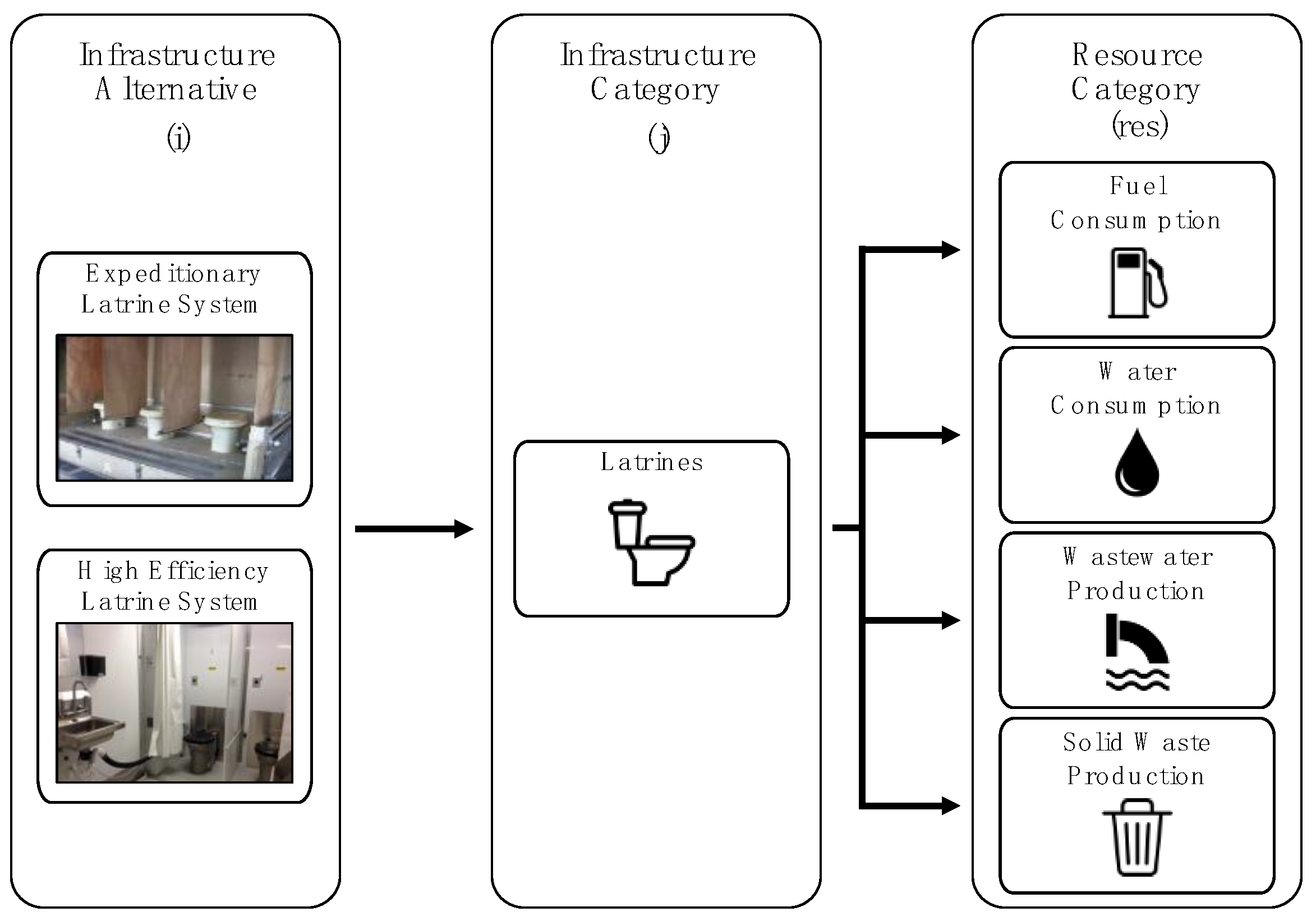
2.1. Decision Variables

The decision variables utilized in the present model are designed to represent feasible alternatives for enhancements to remote community infrastructure categories that impact sustainability objectives. The model considers various infrastructure alternatives, i, within infrastructure categories, j. The present model considers 11 infrastructure categories, including facility insulation, billeting, power production, water production, food preparation, refrigeration, laundry services, hygiene services, latrines, wastewater management, and solid waste management. These infrastructure categories were selected due to their direct impact on the key resource categories of fuel, water, wastewater, and solid waste. Each alternative is represented by an integer value, i. The model incorporates these alternatives into J infrastructure categories, where each alternative within category j fulfills the same support requirement. Site designers may select any one alternative per infrastructure category, so long as the same level-of-service constraint is achieved. A benefit of the model is its flexibility; it can be adapted for any number of infrastructure alternatives or categories.

For example, Figure 1 depicts the flexibility a planner has to select either an expeditionary or high-efficiency latrine system alternative. One alternative must be chosen to meet the community’s latrine requirement. The latrine infrastructure category is of concern due to its impact on all four resource categories, including fuel consumption, water consumption, wastewater production, and solid waste production.

2.2. Metric Identification

The model was designed to minimize negative sustainability impacts by generating optimal tradeoffs between two competing objectives: (1) minimizing negative environmental impacts; and (2) minimizing life-cycle cost.

2.2.1. Environmental Impact Metric

The model’s first metric is formulated to quantify the impact that remote community infrastructure has on the surrounding environment. While there are various approaches to quantifying environmental impact, greenhouse gas (GHG) emissions are of primary concern due to their influence on climate change. Of the GHGs, carbon dioxide (CO₂) is the largest direct source of radiative forcing from human activities, and it is, therefore, the baseline by which global warming potential is defined [26,27]. The environmental impact of an infrastructure alternative over its lifespan is calculated as the sum of its initial environmental impact (IEI) and its ongoing daily environmental impact (DEI) (metric tons CO₂e). Accordingly, the environmental impact (EI_p) of a portfolio of alternatives is a summation of each alternative’s EI, as shown in Equation (1). Each portfolio represents some combination of infrastructure alternatives where one alternative, i, is selected for each infrastructure category, j. The quantity of portfolios represents all possible combinations of alternatives, calculated as a product of the number of available infrastructure alternatives (I) within each infrastructure category (J)

$$minimize E{I}_p\left(t\right)={\displaystyle \sum }_{j=1}^J\left(IE{I}_{ij}+tDE{I}_{ij}\right)$$

(1)

where

• EI = environmental impact of infrastructure portfolio (tons CO₂e);
• IEI = initial environmental impact of infrastructure alternative (tons CO₂e);
• DEI = daily environmental impact of infrastructure alternative (tons CO₂e/day);
• t = time (days);
• i = infrastructure alternative;
• j = infrastructure category;
• J = total infrastructure categories; and
• p = portfolio of alternatives: one alternative per infrastructure category.

An alternative’s IEI accounts for the impact of its delivery to the site via air, rail, or sea, as shown in Equation (2)

$$IE{I}_{ij}=r^{mode}{w}_{ij}{d}^{mode}$$

(2)

where

• r = emissions rate of transportation mode (tons CO₂e/ton cargo/km) [28];
• mode = mode of transportation (air, land, or sea);
• w = weight of infrastructure alternative (tons); and
• d = transportation distance (km).

The DEI of infrastructure alternative i in category j may be calculated as a function of its daily impact due to each resource category and the resulting transportation requirement, shown in Equation (3). The resource categories of consideration are fuel consumption, water consumption, wastewater production, and solid waste production. The transportation requirement resulting from these resources is further complicated by the tendency of remote communities to utilize readily available, inefficient vehicles to transport resources on- and off-site at varying distances (d). Therefore, Equation (3) also accounts for fluctuations in vehicle capacity (c) and fuel economy (f)

$$DE{I}_{ij}={\displaystyle \sum }_{res=1}^4\left(v_{ij}^{res}{r}_{ij}^{res}\right)+r^{fuel}{\displaystyle \sum }_{res=1}^4\left(\frac{v_{ij}^{res}}{c^{res}}·\frac{d^{res}}{f^{res}}\right)$$

(3)

where

• v = volume of resources (kg/day or L/day);
• res = resources, 1: fuel, 2: potable water, 3: wastewater, and 4: solid-waste;
• r = emissions rate of resource (tons CO₂e/kg or tons CO₂e/L) [29];
• c = carrying capacity of vehicle (kg or L); and
• f = efficiency of vehicle transporting resources (km/L).

2.2.2. Cost Metric

The second metric was formulated to compute an infrastructure portfolio’s life-cycle cost (C_p) from procurement through termination of operations via Equation (4)

$$minimize C_p\left(t\right)={\displaystyle \sum }_{j=1}^J\left(I{C}_{ij}+tD{C}_{ij}\right)$$

(4)

where

• C = life-cycle cost of infrastructure portfolio ($);
• IC = initial cost of alternative ($); and
• DC = daily cost of alternative ($/day).

An alternative’s IC is a function of its procurement cost (PC) and the cost to transport it to the community’s location, as shown in Equation (5) The transportation cost is dependent upon the operating cost (OC) of the transportation method and the number of trips required

$$I{C}_{ij}=P{C}_{ij}+O{C}_{ij}^{mode}{d}_{ij}^{mode}\frac{w_{ij}}{c_{ij}^{mode}}$$

(5)

where

• PC = cost to procure alternative or initiate service ($); and
• OC = operating cost of transportation mode ($/km).

While most infrastructure alternatives have an associated equipment procurement cost, many non-infrastructure alternatives do not. Rather, these have resource purchase costs and daily service fees. Therefore, an alternative’s DC is computed as a function of daily service costs (SC) and resource transportation costs, as shown in Equation (6). Transportation costs are dependent upon the capacity (c) and efficiency (f) of the vehicle transporting each resource type, as well as the distance traveled (d). Further, cost structures are variable. Daily transportation costs may be considered separately, or they may be combined into the service cost. While the contract type shown here is relatively simple, planners have the ability to easily insert their own contract structures

$$D{C}_{ij}={\displaystyle \sum }_{res=1}^4\left(v_{ij}^{res}S{C}_{ij}^{res}\right)+S{C}^{fuel}{\displaystyle \sum }_{res=1}^4\left(\frac{v_{ij}^{res}}{c^{res}}·\frac{d^{res}}{f^{res}}\right)$$

(6)

where SC = service or purchase cost of resource ($/kg or $/L).

2.3. Objective Function

Finally, minmax normalization is applied to the metrics from Equations (1) and (4), as shown in Equations (7) and (8), respectively. This action transforms sustainability metric data into unitless values ranging from zero to one, where zero represents the minimum EI or C of all available infrastructure portfolios and one represents the maximum. The normalizing function enables variables of dissimilar units to be computed into a unitless index

$$E{I}_p^{norm}\left(t\right)=\frac{E{I}_p\left(t\right)-\min \left(EI\right)}{\max \left(EI\right)-\min \left(EI\right)}$$

(7)

$$C_p^{norm}\left(t\right)=\frac{C_p\left(t\right)-\min \left(C\right)}{\max \left(C\right)-\min \left(C\right)}$$

(8)

where

• EI^norm = normalized environmental impact of an infrastructure portfolio; and
• C^norm = normalized cost of an infrastructure portfolio.

Additionally, weights, wt_EI and wt_C, are identified to represent the priority a decision-maker places on each metric in the final optimization function. Both are represented by percentages that must sum to 100 percent. Finally, the objective function shown in Equation (9) is utilized to calculate an infrastructure portfolio’s negative sustainability impacts, SI_p, and identify an optimal portfolio for any time, t, based on the decision-maker’s priorities. For the purposes of this research effort, the optimal solution is defined as that portfolio which minimizes negative impacts on sustainability objectives.

$$minimize S{I}_p\left(t\right)=w{t}_{EI}E{I}_p^{norm}\left(t\right)+w{t}_C{C}_p^{norm}\left(t\right)$$

(9)

where

• wt_EI = importance weight of environmental impact;
• wt_C = importance weight of cost; and
• SI = negative sustainability impacts of an infrastructure portfolio.

3. Model Input Data

Remote community planners must input a number of community features, planning factors, and infrastructure alternative characteristics, as outlined in

Table 1. Model input data.

Input Category	Inputs
Community Features	(1) required personnel (persons) (2) environment (e.g., desert, temperate, or tropical) (3) duration (days) (4) equipment delivery method (ground, air, or sea) (5) equipment delivery distance (km) (6) distance to local services (km) (7) transportation method efficiencies (km/L) (8) transportation method capacities (kg or L)
Planning Factors	(1) power consumption (kW/person/day) (2) potable water consumption (L/person/day) (3) solid waste production (kg/person/day) (4) wastewater production (L/person/day)
Infrastructure Alternative Characteristics	(1) fuel consumption (L/day) (2) water consumption (L/day) (3) wastewater production (L/day) (4) solid waste production (kg/day) (5) procurement cost (USD) (6) operating costs (USD) (7) shipping weight (kg) (8) emissions factor (ton CO2/unit)

. Community features describe the community’s location and determine support requirements. Planning factor data establishes the site’s total resource requirement, which is dependent upon location and number of personnel. Finally, feasible alternatives must be identified for each infrastructure category, such as power production, water production, wastewater management, and solid-waste management. For each infrastructure alternative, characteristic data determine the alternative’s resource consumption, waste production, transportation requirement, cost, and environmental impact. Life-cycle boundary conditions were implemented such that negative sustainability impacts were considered from the time of an alternative’s mobilization through operation, while impacts from manufacturing and infrastructure retirement were excluded.

4. Case Study

In order to demonstrate the model, a theoretical military forward operating base (FOB) was designed as a reasonable representation of a remote community, and infrastructure alternatives were considered. A military application was chosen for the following example due to the abundance of bases with remote community characteristics and the breadth of data on sustainable base initiatives. For this case study, a baseline FOB was first modelled as a typical example of deployed military assets. Next, a set of equipment alternatives were modelled to demonstrate potential improvements as a result of investing in sustainable technologies. Then, a set of procedural alternatives were applied to demonstrate potential performance improvements based on currently fielded infrastructure.

For this case study, the required input data included community features, planning factors, and infrastructure alternative characteristics. First, community features were dictated based on the FOB’s design to accommodate 300 personnel in an arid region of Southwest Asia for an anticipated duration of up to 7 years. All equipment technologies (such as generators, solar panels, and water purifiers) had to be delivered via aircraft from suppliers located in Central Europe, 5150 km away. Common services (such as purchasing bottled water or contracting solid waste disposal) could be sourced from local vendors ranging from 40–80 km from the site. The community feature data and assumptions are summarized in

Table 2. Case study community feature summary.

Resource	Variable	Value	Units	Reference
Fuel	Cost (SCfuel)	4	$/L	[6]
	Emissions Rate (rfuel)	2.6 × 10−3	metric tons CO2/L	[29]
	Delivery Distance (dfuel)	65	km
	Vehicle Efficiency (ffuel)	0.8	km/L	[34]
	Vehicle Capacity (cfuel)	18,925	L	[35]
Water	Cost (SCwater)	2.6	$/L	[6]
	Delivery Distance (dwater)	40	km
	Vehicle Efficiency (fwater)	0.7	km/L	[35]
	Vehicle Capacity (cwater)	17,033	L	[35]
Wastewater	Cost (SCww)	0.5	$/L
	Emissions Rate (rww)	2.3 × 10−5	metric tons CO2/L
	Delivery Distance (dww)	80	km
	Vehicle Efficiency (fww)	0.7	km/L	[35]
	Vehicle Capacity (cww)	15,140	L	[35]
Solid Waste	Cost (SCsw)	8.8	$/kg
	Emissions Rate—landfill (rsw)	1.3 × 10−3	metric tons CO2/kg	[36]
	Emissions Rate—burn pit (rsw)	9.9 × 10−4	metric tons CO2/kg
	Emissions Rate—incinerator (rsw)	6.4 × 10−4	metric tons CO2/kg	[36]
	Delivery Distance (dsw)	72	km
	Vehicle Efficiency (fsw)	0.7	km/L	[35]
	Vehicle Capacity (csw)	16.5	tons	[35]
Equipment Alternatives	Cost (OCair)	29	$/km	[37]
	Emissions Rate (rair)	4.1 × 10−4	metric tons CO2/km	[28]
	Delivery Distance (dair)	5172	km
	Aircraft Capacity (cair)	86	tons	[37]

. Second, planning factors were identified for power, water, wastewater, and solid waste through U.S. Army design manuals and historical data [6]. Third, infrastructure alternative data were sourced from a collection of U.S. Army reports published as a result of an initiative to identify fuel, water, and waste (FWW) mitigation measures [30,31,32]. Objectives were computed in R version 3.6.0 [33] and figures were produced with the ggplot2 package [34].

4.1. Baseline

First, a set of baseline FWW values, summarized in

Table 3. Resource summary, 300 personnel, arid environment [31].

Resource Category	Volume	Unit
Fuel Demand	3944	L/day
Power Demand	5108	kWh/day
Potable Water Demand	33,017	L/day
Wastewater Demand	32,282	L/day
Solid Waste Demand	1302	kg/day

, was established through experimental testing of a baseline camp setup [38]. This baseline established a standard by which all other alternatives could be compared. The baseline setup represented commonly deployed assets for billeting, food preparation and dining facilities, hygiene services, waste management, water storage and distribution, and power generation, as shown in

Table 4. Equipment and procedural infrastructure alternative characteristics.

	Infra. Cat.	Infrastructure Alternative	vfuel	vwater	vww	vsw	wt	PC
			(L)	(L)	(L)	(kg)	(kg)	(USD/unit)
Equipment Alternatives		Baseline site	3944	33,017	32,282	1302	506,835	1,191,215
	Facility Insulation	(Baseline Alt.)—Single ply tent liner					3129	23,000
		Insulated tent liner & photovoltaic array shade	3478	33,017	32,282	1302	17,647	487,830
	Power Production	(Baseline Alt.)—60 kW tactical generator					41,929	650,000
		Hybrid generator and battery system	2740	33,017	32,282	1302	241,061	7,200,000
		Photovoltaic array and battery system	397	33,017	32,282	1302	1,015,840	35,600,000
	Food Preparation	(Baseline Alt.)—Expeditionary kitchen system					6349	150,000
		Fuel-fired expeditionary kitchen system	3823	33,304	32,570	1302	6984	170,000
	Refrigeration	(Baseline Alt.)—Multi-temperature refrig. system					18,225	120,000
		High efficiency refrigeration system with solar array	3914	33,017	32,282	1302	17,493	136,150
	Water Production	(Baseline Alt.)—Bottled water imported to site					0	0
		Reverse osmosis water purification system	4148	-4349	32,282	1302	3628	284,500
	Latrines	(Baseline Alt.)—Expeditionary latrine system					11,646	200,000
		High efficiency latrine system	4383	25,401	23,020	1305	13,393	240,000
	Solid Waste Mgmt	(Baseline Alt.)—Waste exported from site to landfill					0	0
		Open-air burn pit	4020	33,017	32,282	160	0	5000
		Incinerator	4008	33,017	32,282	226	38,774	750,000
	Wastewater Mgmt	(Baseline Alt.)—Waste exported from site					0	0
		Activated sludge bioreactor	3952	33,017	3452	1302	12,898	400,000
		Activated sludge bioreactor and reverse osmosis water purification system	3963	15,806	1768	1302	22,571	1,150,000
Procedural Alternatives	Billeting	(Baseline Alt.)—14 personnel per tent					425,292	45,885
		Billeting consolidation, 18 personnel per tent	3732	33,017	32,282	1302	402,436	35,910
	Power Production	(Baseline Alt.)—60 kW tactical generator					38,704	600,000
		Generator reallocation according to avg. loading	3168	33,017	32,282	1302	27,415	425,000
		60 kW tactical generator grid	2324	33,017	32,282	1302	40,316	625,000
	Laundry Services	(Baseline Alt.)—Unlimited laundry allowance					261	2250
		1/2 baseline laundry allowance	3921	31,597	32,282	1302	156	1350
	Hygiene Services	(Baseline Alt.)—10-min daily showers					4	80
		7-min weekly showers	3876	17,998	17,260	1302	4	80
	Latrines	(Baseline Alt.)—Unlimited toilet flushes					11,646	200,000
		Reduced toilet flushes	3936	27,634	26,900	1302	11,646	200,000

. The identified fuel demand included fuel for infrastructure sustainment only—fuel required for transportation outside of the FOB must be accounted for separately. Historical data and subject matter expertise ensured that the baseline infrastructure met U.S. Army requirements for the sustainment of a 300-person contingency site.

The FOB’s baseline environmental impact and cost were calculated using Equations (1)–(3). The initial environmental impact was found to be 2350 tons CO₂e, increasing at a rate of 14.3 tons/day. The capital procurement and mobilization cost was $3.1M, with operating costs of $134,000/day. These values provided a standard by which further infrastructure alternatives may be compared.

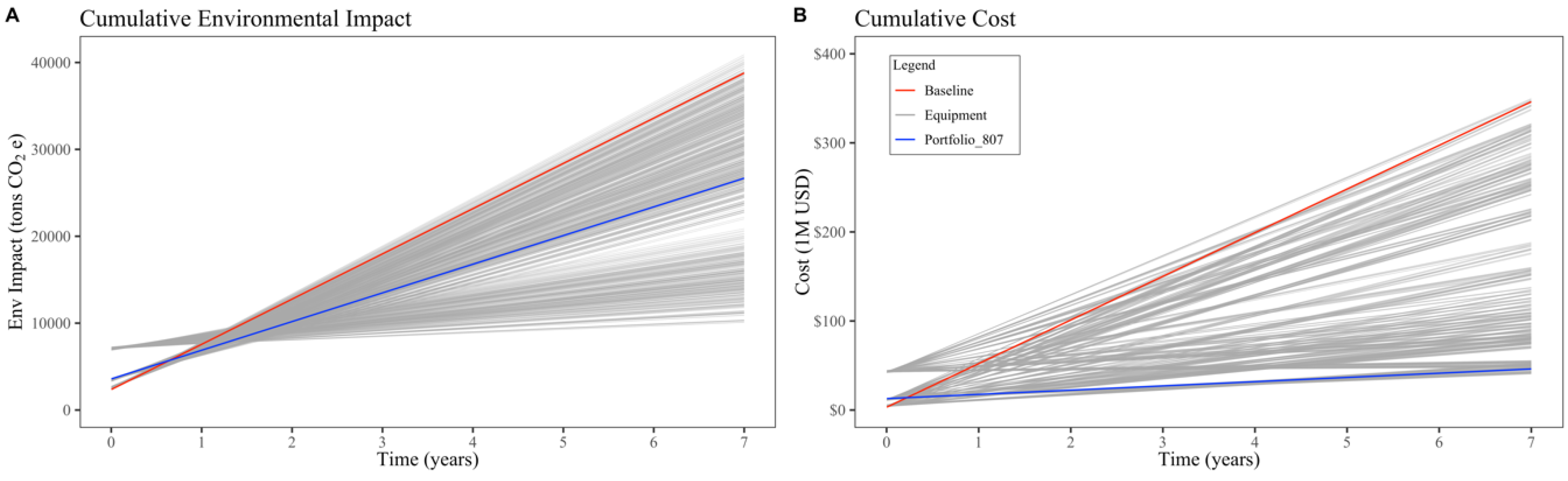
4.2. Equipment Alternatives

Next, the performance of a set of equipment alternatives was modelled. The alternatives and their FWW consumption and production values are detailed in Table 4 as compared to the baseline. The results of this analysis are shown in Figure 2. Each alternative required some material equipment in addition to, or in place of, a baseline equipment set with the potential to conserve resources. Coincidentally, many of these technologies required a substantial investment in terms of the purchase cost and delivery. For example, a photovoltaic array and lithium ion battery system, as a power production alternative, was compared against a baseline of 60 kW generators. While the solar alternative saved the site nearly 3560 liters of fuel per day, the equipment itself weighed over 900,000 kg more than its generator competitor [39]. This extra weight imposed additional delivery costs and transportation emissions.

Figure 2 illustrates the tradeoffs between initial and operating requirements for 864 potential equipment portfolios. Each line represents the cumulative EI and C of one portfolio, with the baseline signified in red. While the baseline equipment set imposed a low IEI and IC, it led to one of the highest possible cumulative EI and C values due to its operating requirements. Other alternatives imposed higher IEI and IC values but lower operating requirements. For example, portfolio #807, shown in Figure 2 as a blue line, was comprised nearly exclusively of sustainable technologies outlined in

Table 5. Baseline versus portfolio #807, an example of sustainable equipment alternatives.

Infrastructure Category	Baseline	Portfolio #807
Fac. Insulation	Single ply tent liner	Single ply tent liner
Power Pro.	60 kW tactical generator	Hybrid generator and battery system
Food Prep.	Expeditionary kitchen system	Expeditionary kitchen system
Refrigeration	Multi-temperature refrigeration system	High efficiency refrigeration system with solar array
Water Pro.	Bottled water imported to site	Reverse osmosis water purification system
Latrines	Expeditionary latrine system	Expeditionary latrine system
Solid Waste Mgmt.	Waste exported from site to landfill	Incinerator
Wastewater Mgmt.	Waste exported from site	Activated sludge bioreactor and reverse osmosis water purification system
Initial EI (CO2e)	2356	3581
Daily EI (CO2e)	14	9
Initial C (USD)	3,100,000	12,900,000
Daily C (USD)	134,000	13,000

. While this portfolio’s IEI and IC were 1.5 and 4.2 times higher than the baseline’s, its operating requirements were 1.6 and 10.3 times lower, respectively. These sustainability tradeoffs resulted in the IC being offset after 81 days and the IEI being offset after 231 days, at which time portfolio #807 became more sustainable than the baseline. Similarly, each interaction in Figure 2 designates the time at which a portfolio became a more environmentally or financially sustainable choice.

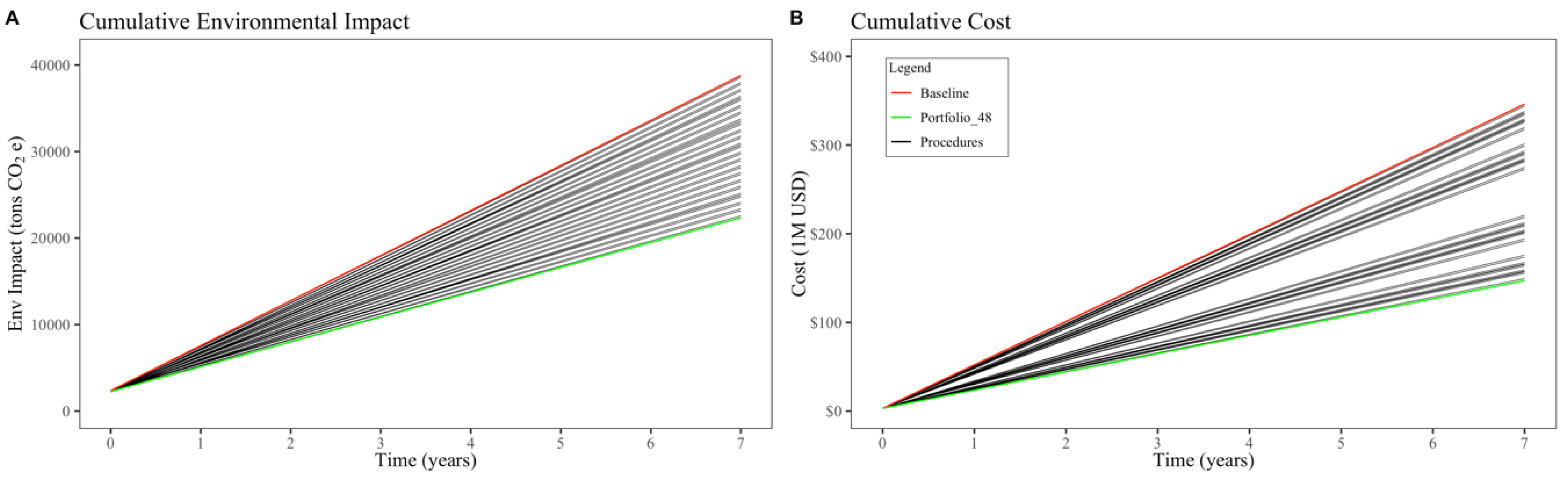
4.3. Procedural Alternatives

In addition to the 864 equipment portfolios, 48 procedural portfolios were also identified through the U.S. Army’s FWW initiative, shown in Table 4 and Figure 3. While the equipment alternatives considered deviations from existing infrastructure, the procedural alternatives utilized only baseline camp equipment. The assessed procedures instead aimed to mitigate resource consumption by restricting personnel quality of life allowances, such as shortening shower times or limiting loads of self-help laundry. For this portion of the case study, each feasible portfolio was comprised of a unique combination of procedural alternatives and evaluated against the baseline. Portfolio #48, the most sustainable set of procedural alternatives, is designated in Figure 3 by a green line. Portfolio #48 was comprised exclusively of resource-saving measures such as billeting consolidation, limited laundry allowances, and reduced shower times and toilet flushes. While these alternatives were not considered in the final optimization function, they did highlight the model’s ability to quantify potential sustainability improvements with a limited equipment investment.

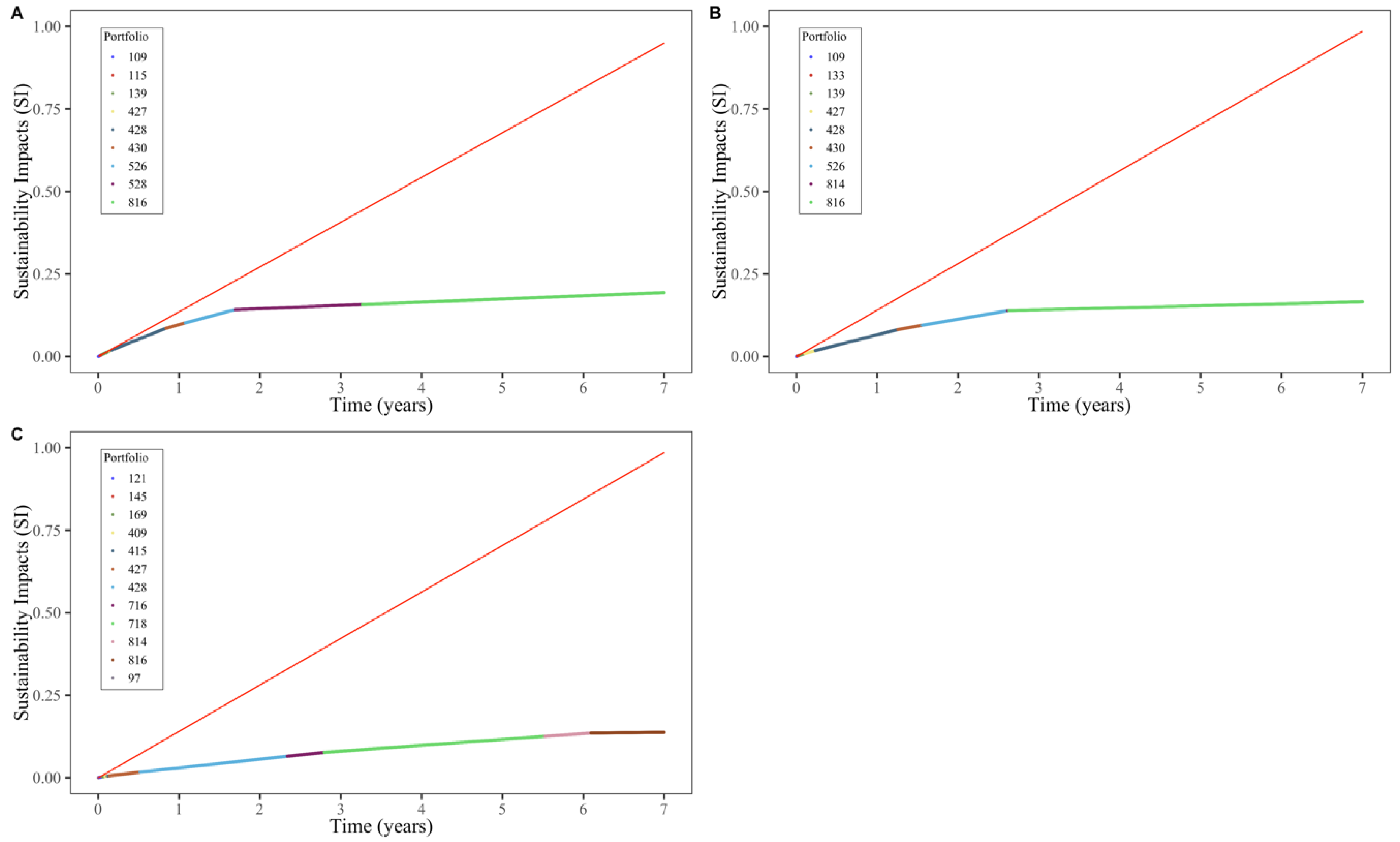
4.4. Optimal Alternatives

Finally, the equipment alternative data were normalized, and the negative sustainability impacts (SI_p) of all equipment-based portfolios were calculated. Then, the optimal solution with the lowest SI at each point in time was identified. Figure 4 shows the optimal portfolios for varying importance weights with the baseline in red for comparison.

In each scenario, the optimal site makeup transitioned rapidly in the first three years. After this point, the optimal site began to steady. In Figure 4a,b, the importance weight applied to the environmental impact was set at 90% and 50%, respectively. In both scenarios, portfolio #816 was found to be the optimal infrastructure alternative combination from 3 years on, due to its low daily emissions of 1.1 CO₂e/day. This site’s makeup included sustainable technologies such as photovoltaic arrays and high efficiency refrigerators and incinerators, as described in

Table 6. Optimal equipment portfolios according to varying importance weights.

Infrastructure Category	Portfolio #816	Portfolio #97
Fac. Insulation	Insulated tent liner and photovoltaic array shade	Single ply tent liner
Power Pro.	Photovoltaic array and battery system	60 kW tactical generator
Food Prep.	Fuel-fired expeditionary kitchen system	Expeditionary kitchen system
Refrigeration	High efficiency refrigeration system with solar array	Multi-temperature refrigeration system
Water Pro.	Reverse osmosis water purification system	Bottled water imported to site
Latrines	Expeditionary latrine system	Expeditionary latrine system
Solid Waste Mgmt.	Incinerator	Open-air burn pit
Wastewater Mgmt.	Activated sludge bioreactor and reverse osmosis water purification system	Waste exported from site
Initial EI (CO2e)	7253	2356
Daily EI (CO2e)	1	14
Initial C (USD)	44,730,000	3,100,000
Daily C (USD)	1500	123,000

. Figure 4c, however, illustrates optimal solutions when the environmental impact importance weight was set at just 10%. In this scenario, the optimal alternative combination changed twice in the fifth year before settling on portfolio #97. Rather than including pricey, environmentally conscious technologies, this site relied on less expensive, easily transportable alternatives that resulted in low procurement and operating costs.

5. Summary and Conclusions

This paper presented a novel infrastructure sustainability assessment model for the design and construction of remote communities. The model was developed in four main sections that included: (1) developing metrics to measure the environmental and economic performance of infrastructure alternatives; (2) formulating the model’s objective functions; (3) identifying the model’s required input data; and (4) testing the model’s performance via a case study. The case study modelled 864 portfolios of feasible infrastructure alternatives and 48 portfolios of procedural alternatives, highlighting that the model is capable of quantifying sustainability impacts for a wide range of decision-maker priorities and infrastructure alternatives. The results also display the model’s effectiveness at identifying the environmental and economic tradeoffs associated with more sustainable, yet more bulky and costly, alternatives. The model was able to generate optimal portfolio solutions according to the importance a planner assigns to the environmental impact and cost metrics. This model has the potential to assist planners by allowing them to identify optimal infrastructure alternatives according to the remote community’s mission, location, and personnel requirements.

This paper presents a model that may be utilized as a framework into which additional sustainability objectives can be incorporated. In this work, the objectives of environmental impact and cost assess the sustainability of infrastructure portfolio decisions, investigating impacts on resource consumption and transportation requirements. While the framework does provide a conduit through which the sustainability of infrastructure systems can be optimized for remote communities, the model presented here is not exhaustive, and future research is necessary. Areas of future research include the optimization of geographical citing according to resource locations, the ability to select multiple alternatives within each category in order to realize synergistic benefits, and the incorporation of additional sustainability objectives such as quality of life, social impact, and human health. Additionally, the present model assumed constant daily resource requirements and emissions factors. Further research should consider a more robust analysis of emissions and operating costs to account for equipment deterioration and irregular maintenance requirements. Additionally, while the presented objective function accounted for the environmental impact and cost from an infrastructure alternative’s purchase through operation, it disregarded production and demolition. Here, it was assumed that all infrastructure alternatives were previously manufactured, which classified their economic impacts as sunk costs. As the remote community’s duration was flexible, the impacts due to demolition or reconstitution were considered negligible. The present model may be adapted to account for these factors.

References

1. Arriaga, M.; Canizares, C.A.; Kazerani, M. Northern Lights: Access to Electricity in Canada’s Northern and Remote Communities. IEEE Power Energy Mag. 2014, 12, 50–59. [Google Scholar] [CrossRef]
2. Cave, G.; Goodwin, W.; Harrison, M.; Sadiq, A.; Tryfonas, T. Design of a sustainable forward operating base. In Proceedings of the 2011 6th International Conference on System of Systems Engineering; IEEE: Albuquerque, NM, USA, 2011; pp. 251–257. [Google Scholar]
3. Arriaga, M.; Canizares, C.A.; Kazerani, M. Renewable Energy Alternatives for Remote Communities in Northern Ontario, Canada. IEEE Trans. Sustain. Energy 2013, 4, 661–670. [Google Scholar] [CrossRef]
4. Anderson, H.G.; Stumpf, A.L.; Rodriguez, G.; Hunter, S.L.; Kinnevan, K. Sustainability Criteria for Contingency Bases; Construction Engineering Research Laboratory; ERDC: Champaign, IL, USA, 2014; p. 96.
5. Akinyele, D.O.; Rayudu, R.K. Strategy for developing energy systems for remote communities: Insights to best practices and sustainability. Sustain. Energy Technol. Assess. 2016, 16, 106–127. [Google Scholar] [CrossRef]
6. Noblis. Sustainable Forward Operating Bases; Strategic Environmental Research and Development Program (SERDP); Defense Technical Information Center: Fort Belvoir, VA, USA, 2010.
7. IPCC. Climate Change 2014: Synthesis Report. Contribution of Working Groups I, II and III to the Fifth Assessment Report of the Intergovernmental Panel on Climate Change; Core Writing Team, Pachauri, R.K., Meyer, L.A., Eds.; Intergovernmental Panel on Climate Change: Geneva, Switzerland, 2014; ISBN 978-92-9169-143-2. [Google Scholar]
8. Putnam, N.H.; Kinnevan, K.J.; Webber, M.E.; Seepersad, C.C. Trucks off the Road: A Method for Assessing Economical Reductions of Logistical Requirements at Contingency Base Camps. Eng. Manag. J. 2016, 28, 86–98. [Google Scholar] [CrossRef]
9. Mao, C.; Shen, Q.; Shen, L.; Tang, L. Comparative study of greenhouse gas emissions between off-site prefabrication and conventional construction methods: Two case studies of residential projects. Energy Build. 2013, 66, 165–176. [Google Scholar] [CrossRef] [Green Version]
10. WNA. Comparison of Lifecycle Greenhouse Gas Emissions of Various Electricity Generation Sources; World Nuclear Association: London, UK, 2011; p. 12. [Google Scholar]
11. Xing, S.; Xu, Z.; Jun, G. Inventory analysis of LCA on steel- and concrete-construction office buildings. Energy Build. 2008, 40, 1188–1193. [Google Scholar] [CrossRef]
12. Racoviceanu, A.I.; Karney, B.W.; Kennedy, C.A.; Colombo, A.F. Life-Cycle Energy Use and Greenhouse Gas Emissions Inventory for Water Treatment Systems. J. Infrastruct. Syst. 2007, 13, 261–270. [Google Scholar] [CrossRef] [Green Version]
13. Vince, F.; Aoustin, E.; Bréant, P.; Marechal, F. LCA tool for the environmental evaluation of potable water production. Desalination 2008, 220, 37–56. [Google Scholar] [CrossRef]
14. El-Fadel, M.; Massoud, M. Methane emissions from wastewater management. Environ. Pollut. 2001, 114, 177–185. [Google Scholar] [CrossRef]
15. Toprak, H. Temperature and organic loading dependency of methane and carbon dioxide emission rates of a full-scale anaerobic waste stabilization pond. Water Res. 1995, 29, 1111–1119. [Google Scholar] [CrossRef]
16. Batool, S.A.; Chuadhry, M.N. The impact of municipal solid waste treatment methods on greenhouse gas emissions in Lahore, Pakistan. Waste Manag. 2009, 29, 63–69. [Google Scholar] [CrossRef] [PubMed]
17. Borglin, S.; Shore, J.; Worden, H.; Jain, R. An overview of the sustainability of solid waste management at military installations. Int. J. Environ. Technol. Manag. 2010, 13, 51. [Google Scholar] [CrossRef] [Green Version]
18. Zhao, W.; van der Voet, E.; Zhang, Y.; Huppes, G. Life cycle assessment of municipal solid waste management with regard to greenhouse gas emissions: Case study of Tianjin, China. Sci. Total Environ. 2009, 407, 1517–1526. [Google Scholar] [CrossRef] [PubMed]
19. Karatas, A.; El-Rayes, K. Optimal Trade-Offs between Housing Cost and Environmental Performance. J. Archit. Eng. 2016, 22, 04015018. [Google Scholar] [CrossRef]
20. Ozcan-Deniz, G.; Yimin, Z.; Ceron, V. Time, Cost, and Environmental Impact Analysis on Construction Operation Optimization Using Genetic Algorithms. J. Manag. Eng. 2012, 28, 265–272. [Google Scholar] [CrossRef]
21. Kamali, M.; Hewage, K.N. Performance indicators for sustainability assessment of buildings. In Proceedings of the International Construction Specialty Conference of the Canadian Society for Civil Engineering (ICSC), Vancouver, BC, Canada, 7–10 June 2015. [Google Scholar]
22. Coello, C.A. Twenty Years of Evolutionary Multi-Objective Optimization: A Historical View of the Field. Evol. Comput. Group. 2005, 20.
23. El-Anwar, O.; El-Rayes, K.; Elnashai, A.S. Maximizing the Sustainability of Integrated Housing Recovery Efforts. J. Constr. Eng. Manag. 2010, 136, 794–802. [Google Scholar] [CrossRef]
24. Poreddy, B.R.; Daniels, B. Mathematical Model of Sub-System Interactions for Forward Operating Bases. In Proceedings of the 2012 Industrial and Systems Engineering Research Conference, Hilton Bonnet Creek, Orlando, FL, USA, 19–23 May 2012. [Google Scholar]
25. Filer, J.; Schuldt, S. Quantifying the Environmental and Economic Performance of Remote Communities. Eur. J. Sustain. Dev. 2019, 8, 176–184. [Google Scholar] [CrossRef]
26. Houghton, J.T.; Jenkins, G.J.; Ephraums, J.J. Climate Change: the IPCC (Intergovernmental Panel on Climate Change) Scientific Assessment; Cambridge University Press: Cambridge, UK, 1990. [Google Scholar]
27. Reilly, J.; Babiker, M.; Mayer, M. Comparing Greenhouse Gases; MIT Joint Program on the Science and Policy of Global Change: Cambridge, MA, USA, 2001; p. 23. [Google Scholar]
28. Chao, C.-C. Assessment of carbon emission costs for air cargo transportation. Transp. Res. Part D Transp. Environ. 2014, 33, 186–195. [Google Scholar] [CrossRef]
29. US EPA. Greenhouse Gases Equivalencies Calculator—Calculations and References. Available online: https://www.epa.gov/energy/greenhouse-gases-equivalencies-calculator-calculations-and-references (accessed on 15 June 2019).
30. Gildea, G.S.; Carpenter, P.D.; Campbell, B.J.; Quigley, J.; Diaz, J.; Langley, J.; Putnam, N.; Hargreaves, B.; Donahue, K.; Lindo, W.; et al. SLB-STO-D Analysis Report: Modeling and Simulation Analysis of Fuel, Water, and Waste Reductions in Base Camps: 50, 300, and 1000 Persons; US Army Natick Solider RD&E Center: Natick, MA, USA, 2017; p. 368.
31. Gildea, G.S.; Carpenter, P.D.; Campbell, B.J.; Quigley, J.; Langley, J.; Putnam, N.; Rinckel, D.; Hargreaves, B.; Lindo, W.; Harris, W.F.; et al. SLB-STO-D: 50, 300, 1000-Person Base Camp, Analysis of FY12 Operationally Relevant Technical Baseline; US Army Natick Solider RD&E Center: Natick, MA, USA, 2017; p. 98.
32. Gildea, G.S.; Carpenter, P.D.; Campbell, B.J.; Harris, W.F.; McCluskey, M.A.; Miletti, J.A. SLB-STO-D: Selected Technology Assessment; US Army Natick Solider RD&E Center: Natick, MA, USA, 2018; p. 226.
33. R Core Team. R: A Language and Environment for Statistical Computing; R Core Team: Vienna, Austria, 2019. [Google Scholar]
34. Wickham, H. ggplot2: Elegant Graphics for Data Analysis; Springer: New York, NY, USA, 2016; ISBN 978-3-319-24277-4. [Google Scholar]
35. Oshkosh Heavy Tactical Vehicles. Available online: https://oshkoshdefense.com/heavy-tactical-vehicles/ (accessed on 4 January 2020).
36. Cherubini, F.; Bargigli, S.; Ulgiati, S. Life cycle assessment (LCA) of waste management strategies: Landfilling, sorting plant and incineration. Energy 2009, 34, 2116–2123. [Google Scholar] [CrossRef]
37. Ritsick, C. C-17 Facts: Everything You Need To Know. Available online: https://militarymachine.com/c-17-facts/ (accessed on 20 June 2019).
38. Harris, W.F., III; Gildea, G.S.; Carpenter, P.D.; Campbell, B.J.; Benasutti, P.B.; Turner, A.J.; Krutsch, M.C.; Miletti, J.A. SLB-STO-D: Demonstration #2—300-Person Camp Demonstration; US Army Natick Solider RD&E Center: Natick, MA, USA, 2017; p. 221.
39. Thomsen, N.; Wagner, T.; Hoisington, A.; Schuldt, S. A sustainable prototype for renewable energy: Optimized prime-power generator solar array replacement. Int. J. Energy Prod. Manag. 2019, 4, 28–39. [Google Scholar] [CrossRef] [Green Version]
Figure 1. Example of decision variables impacting resource categories.
Sustainability 12 02208 g001
Figure 2. The initial impact of alternatives may be offset by low operating requirements.
Sustainability 12 02208 g002
Figure 3. Procedural alternatives result in lower environmental impacts and costs due to negligible investment requirements.
Sustainability 12 02208 g003
Figure 4. Optimal portfolios according to varying importance weights: (a) wtEI = 90%, wtC = 10%; (b) wtEI = 50%, wtC = 50%; and (c) wtEI = 10%, wtC = 90%.
Sustainability 12 02208 g004