Residential Energy-Related CO₂ Emissions in China’s Less Developed Regions: A Case Study of Jiangxi

Abstract

The residential sector is the second-largest consumer of energy in China. However, little attention has been paid to reducing the residential CO₂ emissions of China’s less developed or undeveloped regions. Taking Jiangxi as a case study, this paper thus aims at fully analyzing the difference of the residential energy-related CO₂ emissions between urban and rural regions based on the Log-Mean Divisia Index (LMDI) and Tapio decoupling model. The main results are showed as follows: (1) Since 2008, residential energy-related CO₂ emissions have increased rapidly in both urban and rural Jiangxi. From 2000 to 2017, the residential energy-related CO₂ emissions per capita in rural regions rapidly increased and exceeded that in urban regions after 2015. Furthermore, the residential energy structures had become multiple in both urban and rural regions, but rural regions still had room to optimize its energy structure. (2) Over the study period, consumption expenditure per capita played the dominant role in increasing the residential energy-related CO₂ emissions in both urban and rural regions, followed by energy demand and energy structure. Energy price had the most important effect on decreasing the urban and rural residential energy-related CO₂ emissions, followed by the carbon emission coefficient. However, urbanization increased the urban residential energy-related CO₂ emissions but decreased the CO₂ emissions in rural regions. Population made marginal and the most stable contribution to increase the residential energy-related CO₂ emissions both in urban and rural regions. (3) Overall, the decoupling status showed the weak decoupling (0.1) and expansive negative decoupling (1.21) in urban and rural regions, respectively.

1. Introduction

The Intergovernmental Panel on Climate Change (IPCC) suggests that climate change is a great threat for human survival and development owing to the anthropogenic greenhouse gas (GHG) emissions [1,2]. Since 2006, China has become the largest CO₂ emitter globally [3]. Currently, its emissions account for approximate one third of the global total emissions [4,5]. In this context, China has made commitments and formulated a series of policies to reduce emissions. Meanwhile, there is a consensus that reducing the fast increase of residential CO₂ emissions is a significant pathway to achieve energy-saving and emission-reduction targets in China [6,7]. For China, the residential sector is the second-largest energy consumer category as well as primary CO₂ emissions source [8,9]. Specifically, the residential sector is responsible for 11.7% of energy consumption and 12.6% of CO₂ emissions in 2015 [10]. On one hand, after 40 years of “reform and opening up”, China steps into the new development phase. In addition, with its further development of urbanization and industrialization, the residential CO₂ emissions are expected to increase continuously. Thus, it is necessary and significant to study the key driving forces to help raise reasonable and effective mitigation policies to combat climate change [9]. On the other hand, it is widely appreciated that investment, consumption and export are the troika for economic growth, and it is not wise to simply restrain consumption to mitigate the CO₂ emissions [11]. In addition, as reported by a recent study that China’s economic prosperity had been coupled with environmental degradation, and suggested that decoupling economic growth from ecological impact had been central to achieve the national sustainable development [12]. Therefore, it is also necessary and imperative for China to discover a green, low-carbon and sustainable path to coordinate the link between developmental and environmental protection [13].

In reality, plenty of studies have been conducted to respond to the above concerns for decades in China. They often focused on exploring influencing factors of the CO₂ emissions or energy consumption in the residential sector, based on national or regional perspectives, or analyzing the relationship between economic growth and CO₂ emissions from residential sector. When exploring the drivers affecting residential CO₂ emissions or energy consumption, many factors such as income [14,15,16], population [9,11,17], urbanization [18,19], energy intensity (or energy price) [10,20,21], energy structure [6,22,23], floor space (per capita) [24,25], education level [26], etc., were discussed. For example, based on structural decomposition analysis (SDA), Zhu, et al. [11] studied the indirect residential CO₂ emissions during the period 1992–2005. They argued that population size was not the main reason for the emissions growth anymore, although it promoted the indirect emissions to a certain extent. Using Log-Mean Divisia Index (LMDI), Zhao, et al. [27] decomposed the residential energy consumption in urban China from 1998–2007 at a disaggregated product level. The results demonstrated that energy price had the positive effect on the emission reduction, while population and income played the key role in the growth of the CO₂ emissions. Simultaneously, more scholars were also awareness of the urban–rural gap or dual society in China, thereby they attempted to research Chinese residential CO₂ emissions or energy consumption based on the perspective. Based on Sato–Vartia index, Liu, et al. [17] analyzed the impact of China’s increased urban and rural residential consumption on CO₂ emissions from 1992–2007. Furthermore, Fan, et al. [6] studied the residential CO₂ emissions evolutions in urban–rural divided China and explored the underlying driving forces from the perspective of end-use and behavior by applying Adaptive Weighting Divisia (AWD) decomposition. With the further study on the issue, some researchers extended their scopes and took into account Chinese regional disparity in their related studies. Taking Guangdong, the most developed province in China, as a case study, Wang, et al. [21] decomposed the influencing factors of direct residential energy-related CO₂ emissions into eight factors by using LMDI. The results showed that residential living standard had the largest contribution to the increase of CO₂ emissions, while energy price was the first inhibiting factor. Similarly, taking Liaoning, a coastal province in northeastern China, as an example, Tian, et al. [9] explored the driving forces of the residential CO₂ emissions from 2002–2007 based on LMDI. The results suggested that population and per-capita consumption were the main factors to the increase of residential CO₂ emissions, whereas carbon intensity had the negative effect on the residential CO₂ emissions growth. Moreover, based on spatial–regional level, Yuan, et al. [22] applied LMDI to analyze the drivers of urban and rural residential CO₂ emissions in China’s 30 provinces between 2007 and 2012. They found that population and income-per-capita effects were the main drivers of high urban residential CO₂ emissions in most of the coastal provinces. There were so many studies conducted in many other regions of China. The explanations for these studies can be similarly illustrated, here; we condense some explanations and list some presentative references in

Table 1. Summary of representative studies on investigating the driving forces of Chinese residential sector.

Literature	Region	Scale	Urban–Rural Disparity	Methods
Zha, et al. [14]	China	Nationwide	√	LMDI
Liu, et al. [17]	China	Nationwide	√	Sato–Vartia index
Zhu, et al. [11]	China	Nationwide	×	SDA
Fan, et al. [6]	China	Nationwide	√	AWD
Wang, et al. [21]	Guangdong	Provincial	√	LMDI
Tian, et al. [9]	Liaoning	Provincial	√	LMDI
Bai, et al. [18]	64 cities of Chinese urban agglomerations	City	×	IPAT
Shi, et al. [10]	China and its 30 provinces	Nationwide and Provincial	×	Temporal and spatial LMDI
Yuan, et al. [22]	China’s 30 provinces	Nationwide and Provincial	√	Spatial LMDI

to save space.

In the analysis of the pathway to coordinate CO₂ emissions and economic growth, numerous studies were performed using the decoupling analysis. Generally, there are two main decoupling methods, i.e., OECD indicator and Tapio decoupling indicator [28,29]. Compared with OECD indicator, the latter was more accurate and flexible, which greatly improved OECD indicator. Therefore, Tapio decoupling indicator was more popular and widely used to analyze the relationship between CO₂ emissions and economic growth. In addition, in China, most of these previous studies focused on the main emission sectors: industry [13,30]; transportation [31,32]; construction [33,34]; agriculture [35,36]. To the best of our knowledge, a few scholars applied the Tapio decoupling indicator to analyze the nexus between CO₂ emissions and economic growth from the residential sector. Based on the Tapio decoupling indicator, Ye, et al. [20] conducted the study to analyze the relationship between residential CO₂ emissions and economic growth in China from 1994–2012, which ignored the regional disparity and urban–rural gap. Using the OECD indicator, Yuan, et al. [22] studied the decoupling status in China’s 30 provinces from the residential sector with little content.

Therefore, from Table 1, we can conclude that to date, researchers have mainly focused on developed regions especially coastal provinces and cities such as Guangdong, Liaoning, Jiangsu, Shandong and urban agglomerations, or on national and its 30 provinces when they conducted the studies on exploring the driving forces of CO₂ emissions in the residential sector. Moreover, few studies were conducted on decoupling analysis of the relationship between CO₂ emissions and economic growth from the residential sector compared with other main sectors. The existing related decoupling analysis studies on the residential sector were far from straightforward. As we all know, there is a consensus that China is a multiple-regional and heterogeneous country with the regional disparity and urban-gap [10,23], such as socio-economic, consumption pattern, urbanization, natural resource endowment, energy use, etc. Indeed, China’s mitigation targets need all regions’ efforts. However, this country’s less developed and underdeveloped regions have not yet received academic attention, and few findings can be found in the existing studies worldwide. It is thus crucial to study these less developed and undeveloped regions. This can complete CO₂ emissions profile and help those regions’ decision-makers make reasonable mitigation policies on residential sector by fully considering the local situations.

Under such a circumstance, this paper aims to make up for the above-mentioned deficiencies by fully considering urban–rural gap and regional disparity; we take Jiangxi, a typical less developed province in central China, as a case study. Figure 1 shows its location. Jiangxi is in central China with an administrative area of 166,900 km². Statistically, its total gross domestic product (GDP) reached 2001 billion RenMinBi (RMB) in 2017 [37], which ranked 16 among all 31 regions of China. To the best of our knowledge, its capital city, Nanchang, was assigned the task of pursuing a low-carbon economic transformation in China’s first “Low-Carbon Pilot Cities” national project in 2010 [9,38]. More recently, Jiangxi, Fujian, and Guizhou are selected as the first national ecological civilization test beds in 2016, aiming to set up the relatively sound ecological mechanism for China. According to these facts, we can know that Jiangxi had the huge potential of increasing its CO₂ emissions on residential sector with its further development. However, little academic attention was paid to Jiangxi, especially its residential sector. Thus, based on data availability, we first attempt to overview the situation of residential energy-related CO₂ emissions in Jiangxi urban and rural regions. Then, the driving forces affecting the residential energy-related CO₂ emissions in urban and rural regions are explored by using LMDI. In addition, the Tapio decoupling model was applied to analyze the relationship between the residential energy-related CO₂ emissions and economic growth (consumption expenditure). We believe this study has some innovative significance to help this province make mitigation policies and provide important insight for China’s other less developed or undeveloped regions to reduce emissions.

The remainder of this paper is organized as follows: Section 2 depicts the methodology and data description. Results and discussions are given in Section 3. The main conclusions and corresponding policy implications are provided in Section 4.

2. Methods and Data Description

2.1. Estimation of the Residential Energy-Related CO₂ Emissions

The residential energy-related CO₂ emissions was caused by the residential energy consumption, e.g., lighting, cooking, heating, using household appliances and private transport, in addition, including electricity and heat [9]. Along with these activities, quantities of fossil fuels (e.g., coal, oil, natural gas) and secondary energy sources (e.g., electricity, heat) were consumed, which resulted in CO₂ emissions directly. According to IPCC [39], the residential energy-related CO₂ emissions can be calculated by the following equation:

$$C={\displaystyle \sum _i{\displaystyle \sum _j{C}_{ij}}}={\displaystyle \sum _i{\displaystyle \sum _j{E}_{ij}}}\cdot f_j$$

(1)

where i represents the resident type, i.e., urban residents and rural residents. j represents the fuel type. It should be noted that all kinds of fuel types consumed by residents are subdivided into five categories in this study based on China Energy Statistical Yearbook [40], i.e., coal, oil, natural gas, electricity, and heat. Specifically, coal includes raw coal, briquettes, coke oven gas, and other gases. Oil includes gasoline, kerosene, diesel oil, lubricants, liquefied petroleum gas (LPG) and other petroleum products. Natural gas includes natural gas and liquefied natural gas (LNG). $E_{ij}$ denotes energy consumption of the i type resident, $f_j$ denotes the carbon emission coefficient of j fuel type. With reference to Kennedy, et al. [41], carbon emission coefficients of different energy types are listed in

Table A2. CO₂ emission coefficients of different fuel types investigated in this study.

Fuel Type	Carbon Content	Carbon Oxidation	Net Calorific Value	Emission Coefficient
	Unit: (kg/GJ) a	Unit: (%) a	Unit: (TJ/Gg) a	Unit: (t-CO2/t)
Raw coal	25.8	100	20.9	1.977
Briquettes	26.6	100	17.6	1.717
Coke oven gas	12.1	100	16726 b	7.421 c
Other gases	12.1	100	16726 b	7.421 c
Gasoline	20.2	100	43	3.185
Kerosene	19.5	100	44.1	3.153
Diesel oil	20.2	100	43	3.185
Lubricants	20.0	100	40.2	2.948
Other petroleum products	20.0	100	40.2	2.948
Liquefied petroleum gas	17.2	100	47.3	2.983
Natural gas	15.3	100	38931 b	21.84 c
Liquefied natural gas	17.5	100	44.2	2.836

Note: ^a The value is the IPCC recommended value; ^b The unit is KJ/m³; ^c The unit is t-CO₂/10⁴ m³.

. In addition, it is difficult to acquire the carbon emission coefficients of electricity and heat in Jiangxi. In the light of the data of heat can be only found from 2000–2002, which has small influence on the whole results. For this reason, we use China’s corresponding carbon emission coefficients to substitute for Jiangxi’s carbon emission coefficients of heat. With references to Jia, et al. [38], the carbon emission coefficient of heat can be measured as 0.11 t-CO₂/GJ by the equivalent calorific value. As for the carbon emission coefficient of electricity, here, we calculate and list the coefficient in

Table A1. CO₂ emission coefficient of electricity (t-CO₂/10⁴ kwh).

Year	2000	2001	2002	2003	2004	2005	2006	2007	2008
Coefficient	6.493	7.385	6.886	7.117	7.880	7.992	6.958	7.037	6.909
Year	2009	2010	2011	2012	2013	2014	2015	2016	2017
Coefficient	6.640	6.621	6.623	5.561	5.525	5.265	4.898	4.590	4.844

.

2.2. Decomposition Method

Decomposition analysis has been widely applied to explore the impact factors affecting the changes of CO₂ emissions in the economic and environmental field. To date, there are two mainstream factor decomposition methods [25,36], viz., SDA and index decomposition analysis (IDA). Generally, SDA depends on input–output (IO) table and produces more accurate decomposition results. However, the IO tables are not available every year so that SDA has the limitation to the annual analysis. Inversely, IDA is easier to acquire data and more alterative to use aggregated data to analyze any years’ changes [10]. Hence, IDA is widely applied to decompose the driving factors of energy-related CO₂ emissions. In addition, IDA provides many different indexes to choose [38]. In particular, among these indexes, LMDI has the incomparable advantages for its ease of use and no unexplainable residuals [42]. Moreover, it also provides eight effective strategies to handle zero values problem [43]. In view of these advantages, LMDI has been regarded as the most perfect decomposition method and widely used by many researchers [44,45]. Thus, in this paper, we apply the LMDI to explore the influencing factors affecting the residential energy-related CO₂ emissions in Jiangxi urban and rural regions.

The Kaya identity was widely used to reveal the influencing factors of CO₂ emissions. With the further development of the studies, more influencing factors are discussed. According to Kaya [46], the extended determinants of the residential energy-related CO₂ emissions can be expressed as:

$$C={\displaystyle \sum _i{\displaystyle \sum _j{C}_{ij}}={\displaystyle \sum _i{\displaystyle \sum _j\frac{C_{ij}}{E_{ij}}}\cdot \frac{E_{ij}}{E_i}\cdot \frac{E_i}{Y_{ie}}\cdot \frac{Y_{ie}}{Y_i}}}\cdot \frac{Y_i}{P_i}\cdot \frac{P_i}{P}\cdot P$$

(2)

Let $K_{ij}=\frac{C_{ij}}{E_{ij}}$, $E{S}_{ij}=\frac{E_{ij}}{E_i}$, $E{P}_i=\frac{E_i}{Y_{ie}}$, $E{D}_i=\frac{Y_{ie}}{Y_i}$, $C{P}_i=\frac{Y_i}{P_i}$, $U_i=\frac{P_i}{P}$, $P=P$ in Equation (2) can be written as:

$$C={\displaystyle \sum _i{\displaystyle \sum _j{K}_{ij}}\cdot E{S}_{ij}\cdot E{P}_i\cdot E{D}_i\cdot C{P}_i\cdot U_i\cdot P}$$

(3)

where the variables are defined in

Table 2. Definition of variables.

Variables	Definition
C	Total residential energy-related CO2 emissions
Cij	Residential energy-related CO2 emissions of energy j by resident i
Eij	Residential energy consumption of energy j by resident i
Ei	Residential energy consumption of resident i
Yie	Residence expenditure of resident i
Yi	Consumption expenditure of resident i
Pi	Population of resident i
P	Total population of Jiangxi province
Kij	Carbon emission coefficient of energy j by resident i
ESij	Share of energy j in residential energy consumption by resident i
EPi	Residential energy consumption per unit of residence expenditure for resident i
EDi	Share of residence expenditure to consumption expenditure of resident $i$
CPi	Consumption expenditure per capita of resident i
Ui	Share of population of resident i to total population

.

Thereafter, to explore the contribution of the influencing factors to the total CO₂ emissions, next, we use LMDI, and it has two formations, i.e., additive LMDI (LMDI-I) and multiplicative LMDI (LMDI-II). Based on the additive LMDI, the changes of the total CO₂ emissions ($C_{TOT}$) from the baseline period ($C_0$) to the target period ($C_T$) can be decomposed as the following seven effects:

$$\mathsf{\Delta }{C}_{TOT}=C_T-C_0=\mathsf{\Delta }{C}_{K_{ij}}+\mathsf{\Delta }{C}_{E{S}_{ij}}+\mathsf{\Delta }{C}_{E{P}_i}+\mathsf{\Delta }{C}_{E{D}_i}+\mathsf{\Delta }{C}_{C{P}_i}+\mathsf{\Delta }{C}_{U_i}+\mathsf{\Delta }{C}_P$$

(4)

Each effect can be calculated as follows:

$$\begin{array}{l}\mathsf{\Delta }{C}_{K_{ij}}={\displaystyle \sum _i{\displaystyle \sum _j(}{C}_{ij,T}-C_{ij,0})/(\ln C_{ij,T}-\ln C_{ij,0})\cdot (\ln K_{ij,T}-\ln K_{ij,0})}\\ \mathsf{\Delta }{C}_{E{S}_{ij}}={\displaystyle \sum _i{\displaystyle \sum _j(}{C}_{ij,T}-C_{ij,0})/(\ln C_{ij,T}-\ln C_{ij,0})\cdot (\ln E{S}_{ij,T}-\ln E{S}_{ij,0})}\\ \mathsf{\Delta }{C}_{E{P}_i}={\displaystyle \sum _i{\displaystyle \sum _j(}{C}_{ij,T}-C_{ij,0})/(\ln C_{ij,T}-\ln C_{ij,0})\cdot (\ln E{P}_{i,T}-\ln E{P}_{i,0})}\\ \mathsf{\Delta }{C}_{E{D}_i}={\displaystyle \sum _i{\displaystyle \sum _j(}{C}_{ij,T}-C_{ij,0})/(\ln C_{ij,T}-\ln C_{ij,0})\cdot (\ln E{D}_{i,T}-\ln E{D}_{i,0})}\\ \mathsf{\Delta }{C}_{C{P}_i}={\displaystyle \sum _i{\displaystyle \sum _j(}{C}_{ij,T}-C_{ij,0})/(\ln C_{ij,T}-\ln C_{ij,0})\cdot (\ln C{P}_{i,T}-\ln C{P}_{i,0})}\\ \mathsf{\Delta }{C}_{U_i}={\displaystyle \sum _i{\displaystyle \sum _j(}{C}_{ij,T}-C_{ij,0})/(\ln C_{ij,T}-\ln C_{ij,0})\cdot (\ln U_{i,T}-\ln U_{i,0})}\\ \mathsf{\Delta }{C}_P={\displaystyle \sum _i{\displaystyle \sum _j(}{C}_{ij,T}-C_{ij,0})/(\ln C_{ij,T}-\ln C_{ij,0})\cdot (\ln P_T-\ln P_0)}\end{array}$$

(5)

$$L(a,b)=\{\begin{array}{c}(a-b)/(\ln a-\ln b),a\ne b(a>0,b>0)\\ 0,a=b(a>0,b>0)\end{array}$$

(6)

In addition, to present the decomposition results clearer, here, we also use the multiplicative LMDI. According to Shao, et al. [47], the corresponding multiplicative LMDI can be written as:

$$\mathsf{\Psi }{C}_{TOT}=\frac{C_T}{C_0}=\mathsf{\Psi }{C}_{K_{ij}}\cdot \mathsf{\Psi }{C}_{E{S}_{ij}}\cdot \mathsf{\Psi }{C}_{E{P}_i}\cdot \mathsf{\Psi }{C}_{E{D}_i}\cdot \mathsf{\Psi }{C}_{C{P}_i}\cdot \mathsf{\Psi }{C}_{U_i}\cdot \mathsf{\Psi }{C}_P$$

(7)

where $\mathsf{\Psi }{C}_w=\exp \left({\displaystyle \sum _i\frac{\ln {\omega }_T}{\ln {\omega }_0}\cdot \frac{(C_{ij,T}-C_{ij,0})/(\ln C_{ij,T}-\ln C_{ij,0})}{(C_T-C_0)/(\ln C_T-\ln C_0)}}\right)$, and $\omega$ means $K_{ij}$, $E{S}_{ij}$, $E{P}_i$, $E{D}_i$, $C{P}_i$, $U_i$ and $P$. ${\mathsf{\Psi }}_{TOT}$ means the changes of the total CO₂ emissions between the baseline period and the target period with the corresponding multiplicative formation of the LMDI.

To the best of our knowledge, the CO₂ emission coefficient is usually assumed as a constant value, which has no contributions to the changes of CO₂ emissions. However, in this paper, the CO₂ emission coefficient of electricity changes every year, and it will lead to the changes of CO₂ emissions. Therefore, we finally analyze the following seven effects: the carbon emission coefficient effect ($\mathsf{\Delta }{C}_{K_{ij}}$ and $\mathsf{\Psi }{C}_{K_{ij}}$), energy structure effect ($\mathsf{\Delta }{C}_{E{S}_{ij}}$ and $\mathsf{\Psi }{C}_{E{S}_{ij}}$), energy price effect ($\mathsf{\Delta }{C}_{E{P}_i}$ and $\mathsf{\Psi }{C}_{E{P}_i}$), energy demand effect ($\mathsf{\Delta }{\mathrm{C}}_{E{D}_i}$ and $\mathsf{\Psi }{C}_{E{D}_i}$), consumption expenditure per-capita effect ($\mathsf{\Delta }{C}_{C{P}_i}$ and $\mathsf{\Psi }{C}_{C{P}_i}$), urbanization effect ($\mathsf{\Delta }{C}_{U_i}$ and $\mathsf{\Psi }{C}_{U_i}$) and population effect ($\mathsf{\Delta }{C}_P$ and $\mathsf{\Psi }{C}_P$).

2.3. Decoupling Model

The decoupling theory initially originated from the field of physics, which denotes the de-linkage relationship between two or more variables. Organization for Co-operation and Development (OECD) first categorized the decoupling indicators into relative decoupling and absolute decoupling [28]. However, there are some limitations and shortcomings of the OECD decoupling theory. Specifically, it is liable to be affected by the decoupling elasticity and lacked obvious criteria for choosing appropriate factors [36]. In view of this, Tapio [29] subdivided decoupling indicators into eight sub-categories to analyze the relationship between the road traffic and CO₂ emissions in the EU 15 countries from 1970–2001, which greatly improved the framework of OECD decoupling indicators. Since then, the Tapio decoupling model (see

Table 3. Framework of the Tapio decoupling indicators.

Decoupling State	Abbreviation	$\mathsf{\Delta }{\mathbf{C}}_{\mathbf{i}}/{\mathbf{C}}_{\mathbf{i}}^0$	$\mathsf{\Delta }{\mathbf{Y}}_{\mathbf{i}}/{\mathbf{Y}}_{\mathbf{i}}^0$	${\mathit{D}}_{\mathit{i}}$
Strong decoupling	SD	<0	>0	(−∞, 0)
Weak decoupling	WD	>0	>0	(0, 0.8)
Recessive decoupling	RD	<0	<0	(1.2, +∞)
Strong negative decoupling	SND	>0	<0	(−∞, 0)
Weak negative decoupling	WND	<0	<0	(0, 0.8)
Expansive negative decoupling	END	>0	>0	(1.2, +∞)
Expansive coupling	EC	>0	>0	(0.8, 1.2)
Recessive coupling	RC	<0	<0	(0.8, 1.2)

) was widely used to explore the dynamics nexus between economic growth and environmental protection. However, based on the context above, the decoupling analysis of the CO₂ emissions in the residential sector was far from straightforward in China, especially in less developed regions. Therefore, in this paper, the Tapio decoupling model was selected to analyze the decoupling status and the underlying drivers of the residential consumption expenditure from the residential energy-related CO₂ emissions in Jiangxi urban and rural regions.

According to Tapio [29], the decoupling indicator of residential energy-related CO₂ emissions of the $i$ type resident from residential consumption expenditure can be expressed as:

$$D_i=\frac{C_i\%}{Y_i\%}=\frac{\mathsf{\Delta }{C}_i/C_i{}^0}{\mathsf{\Delta }{Y}_i/Y_i{}^0}$$

(8)

2.4. Data Description

Based on data availability, in this paper, the study period ranges from 2000 to 2017. To the best of our knowledge, since 1953, with a gap from 1963 to 1965, Chinese government has formulated plans for national economic and social development every five years, namely “Five-Year Plan (FYP)”. To make the related results and analysis clearer, here, the study period is consistent with the FYP and subdivided into four stages, i.e., 2000–2005 (10th FYP), 2005–2010 (11th FYP), 2010–2015 (12th FYP) and 2015–2017 (13th FYP). In addition, it is noteworthy that Chinese government proposed a new stage, called “the new normal”, of China’s economic development during the 12th FYP, which was coincided with the last two stages.

All residential energy data are collected from Energy Balance Sheet of Jiangxi Province in the China Energy Statistical Yearbook (2001–2018) [40]. The related consumption expenditure per capita and population data directly derive from the Jiangxi Statistical Yearbook (JSY) (2001–2018) [37]. It should be noticed that consumption expenditure is subdivided into eight categories (e.g., food, cigarettes and wine, clothing, residence, household appliances, and services) in the JSY [37]. Additionally, among these categories, the data of residence expenditure (including the expenditure of housing, electricity, water, fuel and others) is the main source of the residential energy-related CO₂ emissions [21]. Thus, we split the residence expenditure from the consumption expenditure to make the analyses clearer. The share of residence expenditure to consumption expenditure is defined the residential energy demand in this study.

3. Results and Discussion

3.1. Overview the Situation of Residential Energy-Related CO₂ Emissions in Urban and Rural Jiangxi

3.1.1. The Trends of Residential Energy-Related CO₂ Emissions

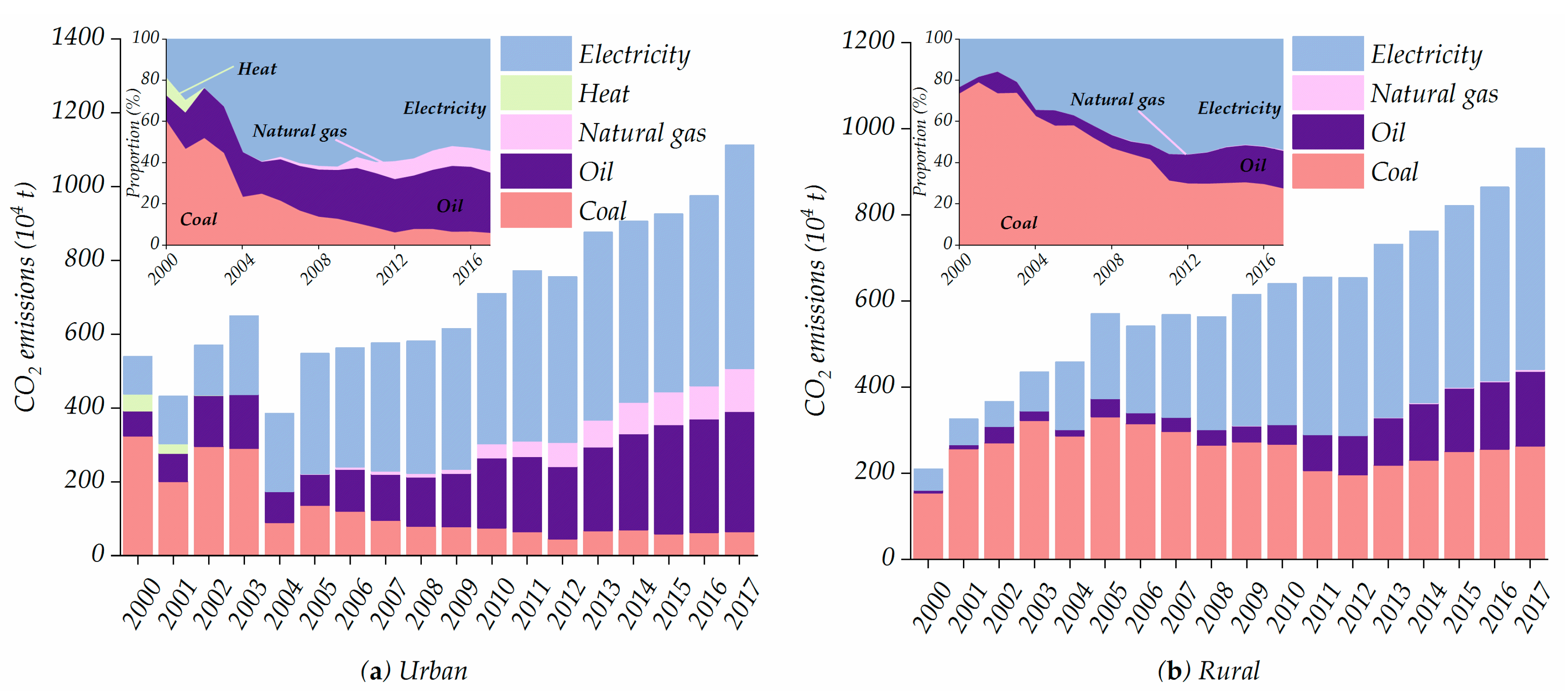
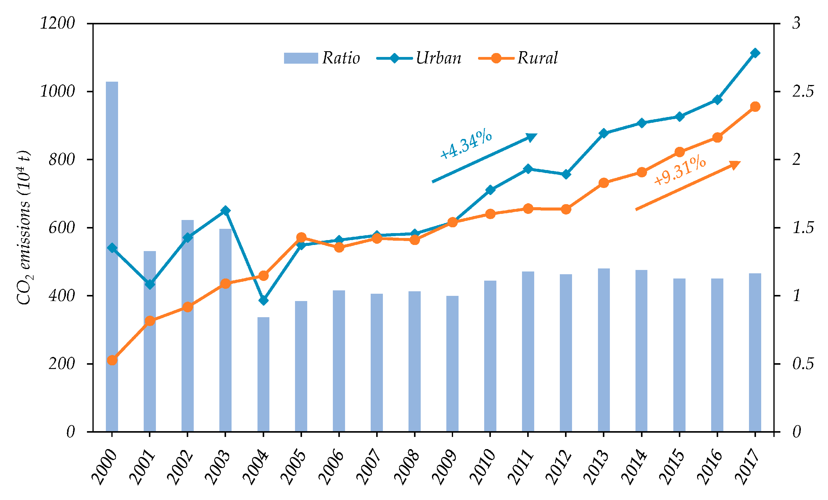
As shown in Figure 2, the urban residential energy-related CO₂ emissions grew from 540.38 × 10⁴ t in 2000 to 1112.84 × 10⁴ t in 2017, with an annual average increase amount of 33.67 × 10⁴ t and a growth rate of 4.34%. The trend of urban residential energy-related CO₂ emissions could be subdivided into three phases: a fluctuating phase (2000–2005), a slow growth phase (2005–2008) and a rapid increase phase (2008–2017). From 2000–2005, it could be easily seen that the urban residential energy-related CO₂ emissions was from 540.38 × 10⁴ t to 548.28 × 10⁴ t, with an annual growth rate of only 0.29%. This phenomenon might be mainly attributed to the large-scale adjustment of the energy structure and cut down the share of coal use. From 2005–2008, because the global economic crisis took place around 2008, people restricted and reduced all kinds of expenditure in daily life, but the consumption of electricity could not fall for people’s habits and customs [38]. Specifically, the urban residential energy-related CO₂ emissions were not more than 600 × 10⁴ t. After 2008, the urban residential energy-related CO₂ emissions grew to 615.17 × 10⁴ t in 2009, then it steadily and quickly increased to 1112.84 × 10⁴ t, with an annual growth rate of 7.47%. The rapid growth of the residential energy-related CO₂ emissions might be explained by the recovery from the crisis and the improvement of economy and living standard for urban residents. This situation was mainly caused by the growing demand of high-carbon appliances and private transport (

Table 4. Urban: Ownership of major durable consumer goods per 100 urban households at year-end.

Item (Unit)	2000	2005	2010	2015	2017
Motorcycle	12.96	24.38	20.77	30.67	29.04
Family car	0.39	0.73	5.31	20.02	29.21
Washing machine	80.15	95.29	93.84	90.68	94.21
Refrigerator	75.82	90.66	96.57	96.64	98.6
Color TV set	106.01	139.31	148	139.13	136.29
Computer	4.56	32.03	59.91	73.98	74.33
Air conditioner	17.07	72.41	107.67	124.31	137.65
Mobile telephone	14.37	136.26	181.18	226.16	235.73
Shower heater	58.02	81.77	92.28	91.99	95.9

), consuming large quantities of oil and electricity [23]. For example, the number of family cars, air conditioners and computers in 2017 reached 40-fold, 1.9-fold and 2.3-fold than that in 2005, respectively.

By contrast, the rural residential energy-related CO₂ emissions grew from 210.13 × 10⁴ t to 954.82 × 10⁴ t between 2000 and 2017 (Figure 2), with an annual growth amount of 43.81 × 10⁴ t and a growth rate of 9.31%. However, the growth rate of rural residential energy-related CO₂ emissions was quicker than that of urban Jiangxi. Here, we also subdivided the rural residential energy-related CO₂ emissions into three phases: a rapid growth phase (2000–2005), a slight decrease phase (2005–2008) and a steadily growth phase (2008–2017). From 2000–2005, the rural residential energy-related CO₂ emissions grew from 210.13 × 10⁴ t to 570.94 × 10⁴ t, with an annual growth rate of 22.13%. This rapid growth may be explained by the increase of coal and electricity use, it was worth noting that coal still played the dominant role in rural residents’ energy use (Figure 3b), leading to 154.64 × 10⁴ t in 2000 and 331.08 × 10⁴ t CO₂ in 2005, respectively. Analogous to the urban residents, the rural residents were also affected by the economic crisis from 2005–2008, making the corresponding CO₂ emissions declined by −1.27%. From 2008–2017, the rural residential energy-related CO₂ emissions increased from 563.69 × 10⁴ t to 954.82 × 10⁴ t, with an annual growth rate of 6.03%.

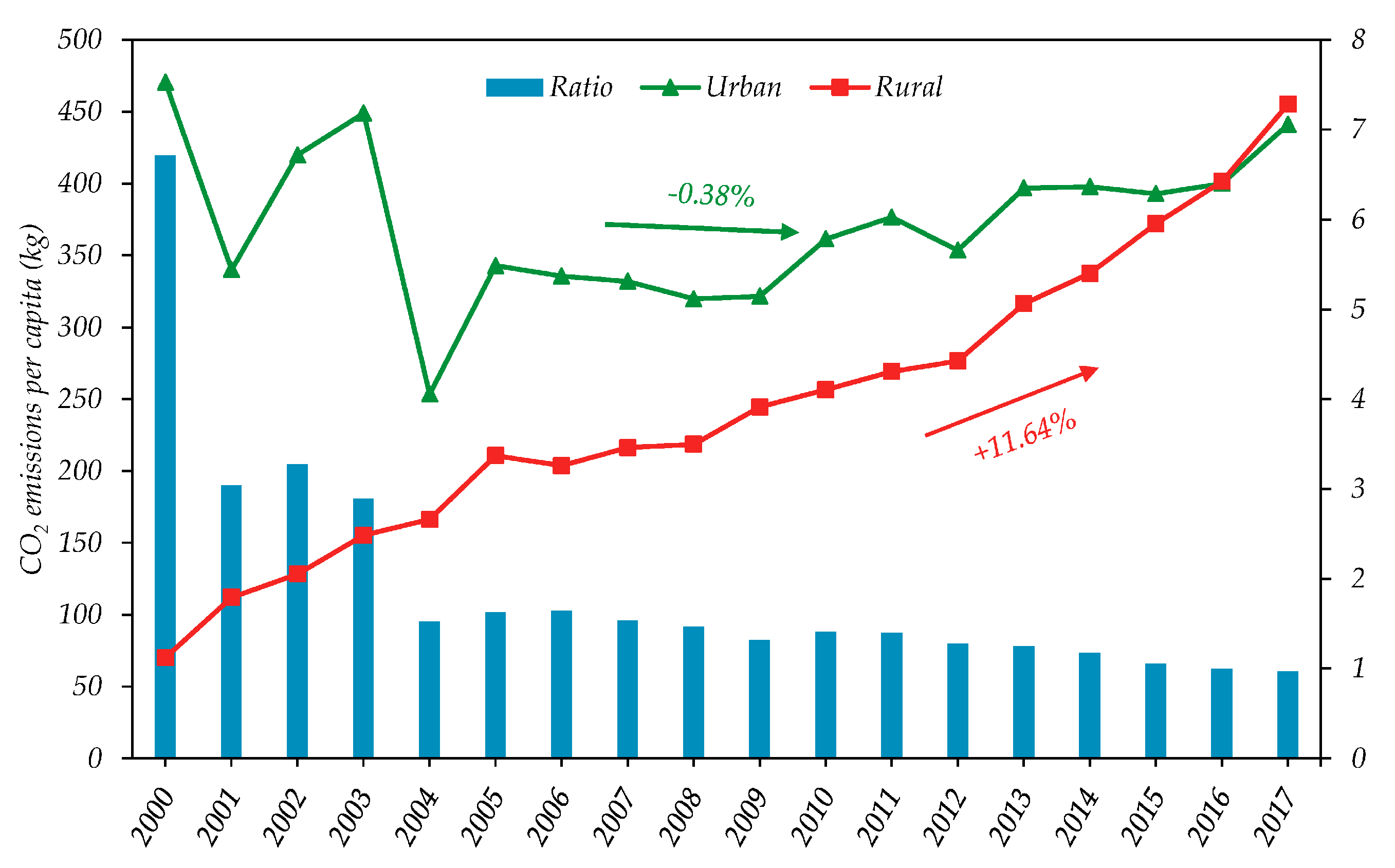
Figure 2 also showed the ratio of the residential energy-related CO₂ emissions for urban and rural regions widened and narrowed, felling from 2.57 in 2000 to 1.17 in 2017. Over the study period, the urban–rural ratio of residential energy-related CO₂ emission most remained the interval 1.0–1.2 except 2000–2005. Specifically, the ratio was more than 1.3 between 2000–2003. To the best of our knowledge, urban residents owned more energy equipment and consumed more commercial energy than that of rural residents, leading to more residential energy-related CO₂ emissions [17,48]. The ratio was 0.84 and 0.96 between 2003 and 2004, respectively. The reason might be that the large-scale reduction of coal use in urban regions as well as the growing popularity of appliances in rural regions (

Table 5. Rural: Ownership of major durable consumer goods per 100 rural households at year-end.

Item (Unit)	2000	2005	2010	2015	2017
Motorcycle	17.47	43.39	60.49	77.41	75.6
Family car	−	−	−	10.59	16.54
Washing machine	3.55	7.02	14.08	43.05	55.25
Refrigerator	3.63	10.53	45.84	84.68	91.42
Color TV set	30.16	82.33	106.86	127.13	132.12
Computer	−	2	5.22	24.19	24.59
Air conditioner	0.04	2	10.24	42.41	56.48
Mobile telephone	1.43	64.82	140.98	233.19	249.52
Shower heater	1.14	4.12	16.33	56.25	68.01

). From 2006–2017, the ratio of urban–rural always over 1.0, which mainly resulted from the development of urbanization.

3.1.2. The Changes of Residential Energy-Related CO₂ Emissions Per Capita

The changes of residential energy-related CO₂ emissions per capita in Jiangxi urban and rural regions were presented in Figure 4. The urban residential energy-related CO₂ emissions per capita decreased from 470.41 kg-CO₂ in 2000 to 440.96 kg-CO₂ in 2017, with an annual average decrease amount of 1.73 kg-CO₂ and a decrease rate of 0.38%. The trends of urban residential energy-related CO₂ emissions per capita could be also subdivided into three stages: a fluctuating decrease stage (2000–2005), a slow growth stage (2005–2010) and a slightly more rapid growth stage (2010–2017). The urban residential energy-related CO₂ emissions per capita experienced a waved decrease from 470.41 kg-CO₂ in 2000 to 342.79 kg-CO₂ in 2005, then it slowly increased to 361.35 kg-CO₂ in 2010. The decrease of the urban residential energy-related CO₂ emissions per capita could be explained by the following reasons. The proportion of high-quality energy types, such as oil, natural gas, and electricity greatly improved due to the shift of energy structure and the improvement of appliances’ energy efficiency [24]. Additionally, urban residents reduced some unnecessary energy consumption when the financial crisis occurred. The urban residential energy-related CO₂ emissions per capita grew from 361.35 kg-CO₂ to 440.96 kg-CO₂ from 2010–2017, this might be explained by the increase of appliances and private transport (Table 4).

By contrast, the rural residential energy-related CO₂ emissions per capita rapidly increased from 70.05 kg-CO₂ to 455.02 kg-CO₂ from 2000–2017 (Figure 4), with an annual average increase amount of 22.65 kg-CO₂ and a growth rate of 11.64%. In particular, the rural energy-related CO₂ emissions per capita were 401.41 kg-CO₂ and 455.02 kg-CO₂ from 2016–2017 which exceeded that of urban regions. Compare to urban regions, the rural residential energy-related CO₂ emissions presented a tedious upward trend. This situation could be explained by the traditional biomass was gradually outpaced by the commercial energy. Moreover, with the improvement of living standards, rural residents had the capacity to pursuit high-quality life, such as buying more energy-intensive appliances and private transport tools (Table 5). However, many of them lacked the consciousness of environmental protection, resulting in more residential CO₂ emissions [49].

As presented in Figure 4, the gap in residential energy-related CO₂ emissions per capita between Jiangxi urban and rural regions decreased from 6.72 to 0.97 from 2000–2017. In addition, it could be divided into two phases: a rapid decrease phase in 2000–2005 and a slow decrease phase between 2005–2017. The approximate reason might be owing to the development of urbanization and the rural economy [23].

3.1.3. Analysis on the Residential Energy-Related CO₂ Emissions Structure

As shown in Figure 3a, the urban residential energy-related CO₂ emissions caused by coal waned from 324.57 × 10⁴ t in 2000 to 65.64 × 10⁴ t in 2007 and its corresponding share decreased from 60.06% to 5.90%, thereby indicating the reduction of coal use in urban regions. In addition, the residential energy-related CO₂ emissions caused by heat also presented a decrease tendency (46.86 × 10⁴ t in 2000 and 2.01 × 10⁴ t in 2017). The reason was that Jiangxi reduced the supply of heat, eventually, cut it off after 2002. See other energy types, electricity, oil, and natural gas overall presented an upward trend. The residential energy-related CO₂ emissions caused by electricity increased from 101.81 × 10⁴ t to 605.55 × 10⁴ t from 2000–2017, the corresponding share increased from 18.84% to 54.42%. It should be noteworthy that the residential energy-related CO₂ emissions induced by electricity exceeded coal and ranked first, which became the most important energy for urban residents after 2004. Since 2007, the residential energy-related CO₂ emissions induced by oil also exceeded the coal and became the second-largest energy type, and its corresponding share grew from 12.42% in 2001 to 29.24% in 2017. It is likely that the private transport increased rapidly (Table 4). However, starting from 2005, urban residents began to use natural gas. The share of residential energy-related CO₂ emissions induced by natural gas increased quickly from 1.09 × 10⁴ t in 2005 to 116.29 × 10⁴ t in 2007, with an annual growth rate of 47.57%, the corresponding share was from 0.2% to 10.45%. Since 2012, the share of residential energy-related CO₂ emissions induced by natural gas exceeded coal. At present, the residential energy-related CO₂ emissions structure was dominated by electricity, followed by oil, natural gas, and coal in urban regions.

The residential energy-related CO₂ emissions caused by heat was not found in rural regions according to JSY [37]. Here, we only considered coal, oil, natural gas, and electricity. As shown in Figure 3b, the residential energy-related CO₂ emissions for rural residents mainly induced by coal, oil, and electricity, which accounted for over 99% over the study period. In 2000, the residential energy-related CO₂ emissions induced by coal ranked the first, followed by electricity and oil. The share of residential energy-related CO₂ emissions induced by coal decreased from 73.59% to 27.52% from 2000–2007. The residential energy-related CO₂ emissions induced by electricity rapidly increased from 49.02 × 10⁴ t to 513.47 × 10⁴ t over the study period, with an annual growth rate of 14.82%. In 2009, the residential energy-related CO₂ emissions induced by electricity exceeded the coal, which might be explained by the growing increase of appliances. From 2009–2017, electricity became the most important energy type of the residential energy-related CO₂ emission for rural residents. For oil, the residential energy-related CO₂ emissions induced by oil occupied from 3.08% in 2000 to 18.25% in 2017. In addition, its share was still lower than the coal, although the share of coal decreased. Therefore, it could be deduced that the energy structure had further space to optimize for rural regions. The residential energy-related CO₂ emissions induced by natural gas was minimal among other energy types, which increased from 0.66 × 10⁴ t to 4.37 × 10⁴ t from 2008–2017. It should be noted that Jiangxi belonged to the “second pipeline of West–East Natural Gas transmission Project (To provide clean energy and shift energy structure in central and south China, the second pipeline of “West–East Natural Gas transmission Project” was launched in February 2008. Specifically, the pipeline went through Xinjiang, Gansu, Ningxia, Shaanxi, Henan, Hubei, Hunan, Jiangxi, Anhui, Jiangsu, Shanghai, Zhejiang, Guangdong, Guangxi, and H.K.)”, thereby leading to the use of natural gas after 2008. With the implementation of the “coal to gas” project, the demand of natural gas of rural regions in Jiangxi might increase rapidly and expand the of share of residential energy-related CO₂ emissions induced by natural gas in the foreseeable future. Correspondingly, the share of the residential energy-related CO₂ emissions induced by coal would fall further. To the best of our knowledge, coal was a type of low-quality energy; the direct combustion of coal indoors was harmful to human health for rural residents, especially for women and children [17], which in turn led to air pollution even aggregated climate change. From the perspective of socio-development, if the energy structure were outdated, it would be bad for the development of rural economy and education due to the vulnerability of Chinese rural regions. To date, the share of residential energy-related CO₂ emissions structure was electricity, coal, oil, and natural gas in sequence for rural regions.

3.2. Decomposition Analysis of Residential Energy-Related CO₂ Emissions at Four Stages

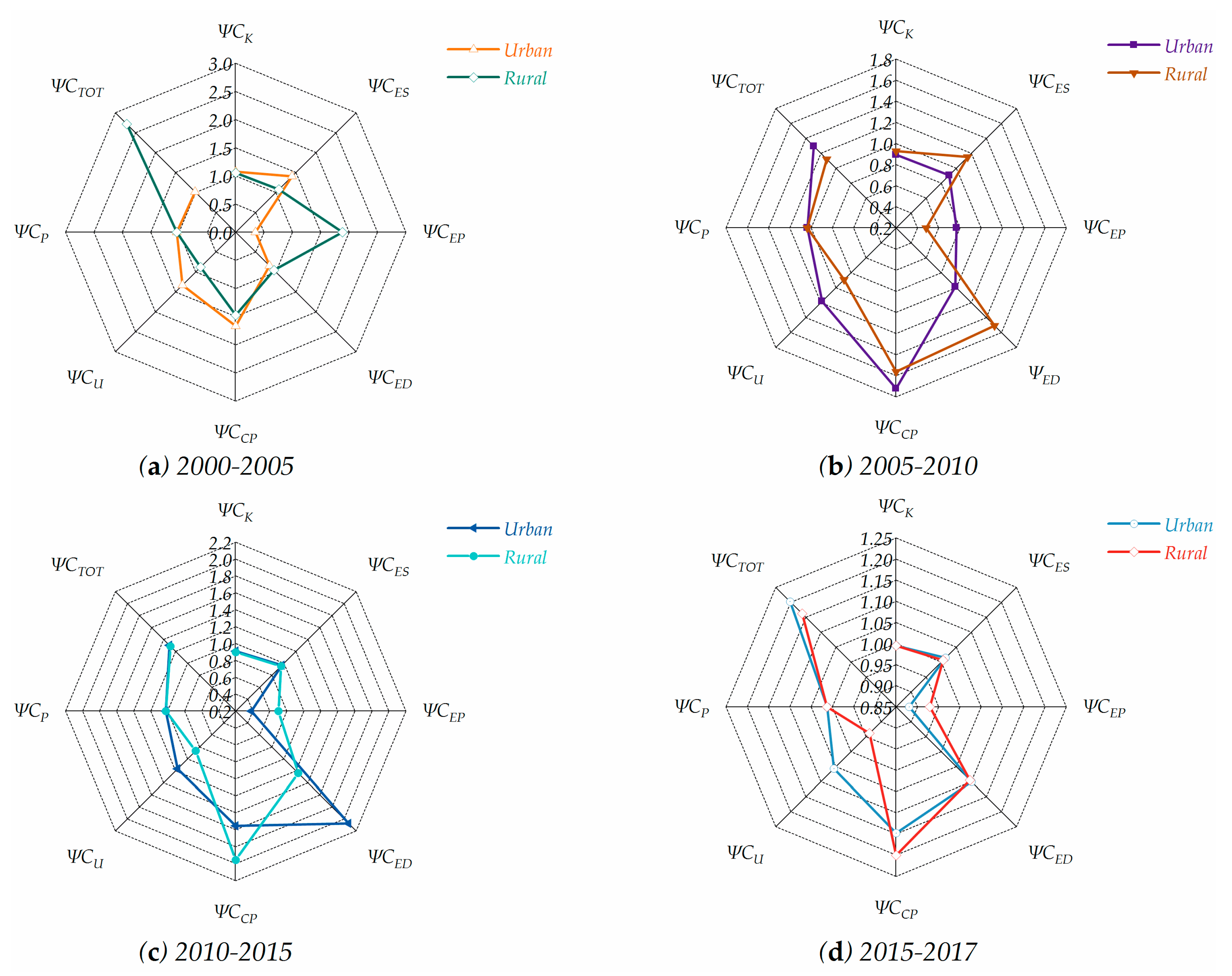
As shown that the urban residential energy-related CO₂ emissions increased by only 7.91 × 10⁴ t with a growth rate of 1.46% during the first stage (Figure 5a and Figure 6a), and then rapidly grew by 162.15 × 10⁴ t with a growth rate of 29.58% in the second stage (2005-2010) (Figure 5a and Figure 6b). During the third stage, the CO₂ emissions increased by 215.42 × 10⁴ t at a rate of 30.32% (Figure 5a and Figure 6c) and grew by 186.98 × 10⁴ t at a rate of 20.19% during the fourth stage (Figure 5a and Figure 6d). Therefore, the conclusion could be drawn that the urban residential energy-related CO₂ emissions presented a sequentially upward trend with a total growth rate of 105.94% over the study period (Figure 5a).

With respect to rural regions, it could be easily observed that the rural residential energy-related CO₂ emissions grew by 360.81 × 10⁴ t at a rate of 171.71% in the first stage (Figure 5b and Figure 6a), and then increased by 69.11 × 10⁴ t at a rate of 12.11% in the second stage (Figure 5b and Figure 6b). During the third and fourth stage, the rural residential CO₂ emissions increased by 181.59 × 10⁴ t with a growth rate of 28.37% (Figure 5b and Figure 6c) and grew by 133.18 × 10⁴ t with a growth rate of 16.21% (Figure 5b and Figure 6d), respectively. Analogous to the urban regions, it could be easily noticed that the rural residential energy-related CO₂ emissions also exhibited a sequentially increasing trend at a rate of 354.39% (Figure 5b).

3.2.1. Consumption Expenditure Per Capita (CE)

To the best of our knowledge, consumption expenditure per capita could reflect folks’ living standards of a region to some extent. As shown in

Table A5. Urban, LMDI multiplicative: Detailed multiplicative decomposition results of the residential energy-related CO₂ emissions of urban residents in Jiangxi.

Periods	$\mathsf{\Psi }{\mathbf{C}}_{\mathbf{T}\mathbf{O}\mathbf{T}}$	$\mathsf{\Psi }{\mathbf{C}}_{\mathbf{K}}$	$\mathsf{\Psi }{\mathbf{C}}_{\mathbf{E}\mathbf{S}}$	$\mathsf{\Psi }{\mathbf{C}}_{\mathbf{E}\mathbf{P}}$	$\mathsf{\Psi }{\mathbf{C}}_{\mathbf{E}\mathbf{D}}$	$\mathsf{\Psi }{\mathbf{C}}_{\mathbf{C}\mathbf{P}}$	$\mathsf{\Psi }{\mathbf{C}}_{\mathbf{U}}$	$\mathsf{\Psi }{\mathbf{C}}_{\mathbf{P}}$
2000–2001	0.80	1.03	1.12	0.55	1.07	1.07	1.09	1.01
2001–2002	1.32	0.98	0.96	1.56	0.73	1.16	1.06	1.01
2002–2003	1.14	1.01	1.06	0.78	1.19	1.08	1.06	1.01
2003–2004	0.59	1.04	1.13	0.54	0.82	1.08	1.04	1.01
2004–2005	1.42	1.01	1.11	0.95	1.11	1.14	1.04	1.01
2005–2006	1.03	0.92	0.97	0.96	1.06	1.09	1.04	1.01
2006–2007	1.02	1.01	1.00	1.00	0.84	1.17	1.03	1.01
2007–2008	1.01	0.99	0.98	0.86	1.04	1.11	1.04	1.01
2008–2009	1.06	0.98	1.01	0.93	0.98	1.11	1.04	1.01
2009–2010	1.15	1.00	0.94	1.01	1.09	1.09	1.02	1.01
2010–2011	1.09	1.00	1.00	1.03	0.91	1.11	1.04	1.01
2011–2012	0.98	0.90	1.06	0.94	0.97	1.09	1.04	1.00
2012–2013	1.16	1.08	0.92	0.41	2.55	1.08	1.03	1.00
2013–2014	1.03	0.97	0.98	1.01	0.95	1.09	1.03	1.00
2014–2015	1.02	0.96	1.02	0.95	0.97	1.09	1.02	1.00
2015–2016	1.05	0.97	1.02	0.96	1.02	1.06	1.03	1.01
2016–2017	1.14	1.03	1.00	0.92	1.08	1.09	1.03	1.01
2000–2005	1.01	1.07	1.40	0.35	0.84	1.67	1.33	1.04
2005–2010	1.30	0.89	0.91	0.77	0.99	1.72	1.18	1.03
2010–2015	1.30	0.91	0.97	0.38	2.08	1.55	1.17	1.02
2015–2017	1.20	0.99	1.01	0.88	1.10	1.15	1.06	1.01
2000–2017	2.06	0.87	1.25	0.09	1.90	5.12	1.94	1.11

, it could be intuitively seen that consumption expenditure per capita always exerted a positive influence on the urban residential energy-related CO₂ emissions, which was in consonance with the results in Figure 5a and

Table 6. Urban: Types and trends of various effects at different stages and average annual contribution rate in Jiangxi urban regions.

Effects	Average Annual Contribution Rate (%)					Trend
	Stage1 a	Stage2 a	Stage 3 a	Stage 4 a	Whole
Total	0.29 b	5.92 b	6.06 b	10.10 b	6.23 b	+++++
Carbon emissions coefficient	1.36	−2.32	−2.22	−0.12	−1.17	+−−−−
Energy structure	6.34	−2.23	−0.82	0.72	1.03	+−−++
Energy price	−20.34	−5.55	−22.02	−6.95	−17.55	−−−−−
Energy demand	−2.72	0.00	16.82	5.29	6.77	−−+++
Consumption expenditure per capita	9.55	11.68	10.24	7.51	11.77	+++++
Urbanization	5.40	3.61	3.54	2.99	4.64	+++++
Population	0.71	0.73	0.51	0.66	0.76	+++++

Note: ^a Stage 1, 2, 3 and 4 refer to 2000–2005, 2005–2010, 2010–2015, and 2015–2017, respectively; ^b is the average annual contribution rate of the total urban residential energy-related CO₂ emissions; + and – stand for positive and negative effect on the CO₂ emissions, respectively.

. Specifically, the additive decomposition effect of consumption expenditure per capita was 257.97 × 10⁴ t in 2000–2005 (Figure 5a and

Table A3. Urban, LMDI additive: Detailed additive decomposition results of the residential energy-related CO₂ emissions of urban residents in Jiangxi (10⁴ t).

Periods	$\mathsf{\Delta }{\mathbf{C}}_{\mathbf{TOT}}$	$\mathsf{\Delta }{\mathbf{C}}_{\mathbf{K}}$	$\mathsf{\Delta }{\mathbf{C}}_{\mathbf{ES}}$	$\mathsf{\Delta }{\mathbf{C}}_{\mathbf{EP}}$	$\mathsf{\Delta }{\mathbf{C}}_{\mathbf{ED}}$	$\mathsf{\Delta }{\mathbf{C}}_{\mathbf{CP}}$	$\mathsf{\Delta }{\mathbf{C}}_{\mathbf{U}}$	$\mathsf{\Delta }{\mathbf{C}}_{\mathbf{P}}$
2000–2001	−107.69	14.76	54.10	−289.23	31.01	33.70	43.79	4.17
2001–2002	137.97	−9.21	−21.85	221.16	−160.11	75.83	27.90	4.25
2002–2003	79.07	5.58	32.87	−151.71	108.15	46.53	33.12	4.52
2003–2004	−263.66	21.64	59.71	−308.42	−102.68	40.65	22.06	3.38
2004–2005	162.23	3.89	46.39	−21.44	50.22	61.27	18.98	2.92
2005–2006	14.70	−44.88	−18.83	−25.26	30.59	46.48	23.04	3.56
2006–2007	13.93	3.77	2.03	−0.89	−101.78	90.94	16.07	3.79
2007–2008	4.81	−6.62	−10.58	−90.45	25.43	61.47	21.52	4.05
2008–2009	33.44	−14.68	5.27	−41.69	−9.63	64.78	25.15	4.24
2009–2010	95.26	−1.10	−39.05	6.03	55.29	56.48	13.19	4.42
2010–2011	61.74	0.14	3.04	24.16	−71.44	74.54	26.97	4.32
2011–2012	−15.90	−79.59	41.95	−49.91	−24.32	63.81	29.53	2.62
2012–2013	120.53	59.95	−71.47	−721.79	762.32	65.28	22.96	3.28
2013–2014	30.29	−24.03	−20.46	12.03	−44.37	79.17	24.06	3.90
2014–2015	18.77	−35.16	17.92	−46.60	−24.62	80.81	22.25	4.17
2015–2016	49.32	−32.32	14.89	−39.66	21.32	52.90	26.70	5.49
2016–2017	137.65	30.07	−1.64	−88.95	76.72	86.19	28.61	6.64
2000–2005	7.91	36.66	171.22	−549.64	−73.42	257.97	145.86	19.25
2005–2010	162.15	−63.51	−61.16	−152.25	−0.11	320.15	98.97	20.06
2010–2015	215.42	−78.69	−29.02	−782.11	597.57	363.61	125.77	18.29
2015–2017	186.98	−2.25	13.25	−128.61	98.05	139.09	55.32	12.14
2000–2017	572.46	−107.79	94.29	−1612.61	622.09	1080.82	425.92	69.74

). Then, from 2005–2010, 2010–2015, and 2015–2017, the decomposition effects were 162.15 × 10⁴ t, 215.42 × 10⁴ t and 186.98 × 10⁴ t (Figure 5a and Table A3). In addition, the consumption expenditure per-capita effect contributed to the largest annual growth rate of the CO₂ emissions (11.77%), and the corresponding average annual contribution rates at four stages were 9.55%, 11.68%, 10.24% and 7.51% (Table 6), respectively. Thus, the conclusion could be drawn that the consumption expenditure per-capita effect played the most important role in promoting the urban residential energy-related CO₂ emissions.

For rural regions, the consumption expenditure per capita also always had a positive effect on the rural residential energy-related CO₂ emissions (Figure 5b and

Table A6. Rural, LMDI multiplicative: Detailed multiplicative decomposition results of the residential energy-related CO₂ emissions of rural residents in Jiangxi.

Periods	$\mathsf{\Psi }{\mathbf{C}}_{\mathbf{T}\mathbf{O}\mathbf{T}}$	$\mathsf{\Psi }{\mathbf{C}}_{\mathbf{K}}$	$\mathsf{\Psi }{\mathbf{C}}_{\mathbf{E}\mathbf{S}}$	$\mathsf{\Psi }{\mathbf{C}}_{\mathbf{E}\mathbf{P}}$	$\mathsf{\Psi }{\mathbf{C}}_{\mathbf{E}\mathbf{D}}$	$\mathsf{\Psi }{\mathbf{C}}_{\mathbf{C}\mathbf{P}}$	$\mathsf{\Psi }{\mathbf{C}}_{\mathbf{U}}$	$\mathsf{\Psi }{\mathbf{C}}_{\mathbf{P}}$
2000–2001	1.55	1.03	0.97	1.37	1.12	1.05	0.96	1.01
2001–2002	1.13	0.99	0.95	1.22	0.97	1.04	0.97	1.01
2002–2003	1.19	1.01	1.06	1.13	0.94	1.07	0.97	1.01
2003–2004	1.05	1.03	1.10	1.06	0.81	1.11	0.98	1.01
2004–2005	1.25	1.01	1.00	0.94	1.16	1.15	0.98	1.01
2005–2006	0.95	0.95	1.06	0.84	1.06	1.08	0.97	1.01
2006–2007	1.05	1.00	1.03	0.83	1.13	1.10	0.98	1.01
2007–2008	0.99	0.99	1.03	0.84	1.07	1.10	0.97	1.01
2008–2009	1.09	0.98	1.03	0.86	1.21	1.07	0.97	1.01
2009–2010	1.04	1.00	1.00	0.97	0.97	1.11	0.98	1.01
2010–2011	1.02	1.00	1.01	0.92	0.95	1.19	0.97	1.01
2011–2012	1.00	0.91	1.03	0.95	1.05	1.10	0.97	1.00
2012–2013	1.12	1.05	0.94	0.72	1.37	1.18	0.97	1.00
2013–2014	1.04	0.97	0.98	1.08	0.93	1.11	0.97	1.00
2014–2015	1.08	0.96	1.00	1.04	0.97	1.14	0.97	1.01
2015–2016	1.05	0.97	1.01	0.95	1.06	1.09	0.97	1.01
2016–2017	1.10	1.03	1.00	0.97	1.03	1.10	0.97	1.01
2000–2005	2.72	1.05	1.08	1.88	0.95	1.47	0.87	1.04
2005–2010	1.12	0.93	1.15	0.48	1.51	1.56	0.89	1.03
2010–2015	1.28	0.90	0.95	0.70	1.24	1.96	0.87	1.02
2015–2017	1.16	0.99	1.01	0.93	1.10	1.20	0.94	1.01
2000–2017	4.54	0.87	1.19	0.59	1.95	5.40	0.63	1.11

). At different four stages, the effect contributed to 166 × 10⁴ t, 258.04 × 10⁴ t, 472.22 × 10⁴ t and 160.16 × 10⁴ t, and the corresponding average annual contribution rates were 15.88%, 9.04%, 14.76% and 9.75% (Figure 5b and

Table 7. Rural: Types and trends of various effects at different stages and average annual contribution rate in Jiangxi rural regions.

Effects	Average Annual Contribution Rate (%)					Trend
	Stage1 a	Stage2 a	Stage 3 a	Stage 4 a	Whole
Total	34.34 c	2.42 c	5.67 c	8.10 c	20.85 c	+++++
Carbon emissions coefficient	1.92	−1.47	−2.40	−0.15	−2.82	+−−−−
Energy structure	3.84	2.79	−1.13	0.31	2.49	++−++
Energy price	18.60	−14.48	−7.27	−3.85	−14.38	+−−−−
Energy demand	−2.43	8.19	4.39	4.78	11.96	−++++
Consumption expenditure per capita	15.88	9.04	14.76	9.75	29.60	+++++
Urbanization	−4.81	−2.34	−3.17	−3.39	−7.69	−−−−−
Population	1.34	0.69	0.50	0.66	1.70	+++++

Note: ^a Stage 1, 2, 3 and 4 refer to 2000–2005, 2005–2010, 2010–2015, and 2015–2017, respectively; ^c is the average annual contribution rate of the total rural residential energy-related CO₂ emissions; + and – stand for positive and negative effect on the CO₂ emissions, respectively.

), respectively. Overall, the average annual led to the largest annual contribution rate (29.60%) over the studied decade, suggesting the effect of consumption expenditure per capita was also the most critical promoting factor to the rural residential energy-related CO₂ emissions.

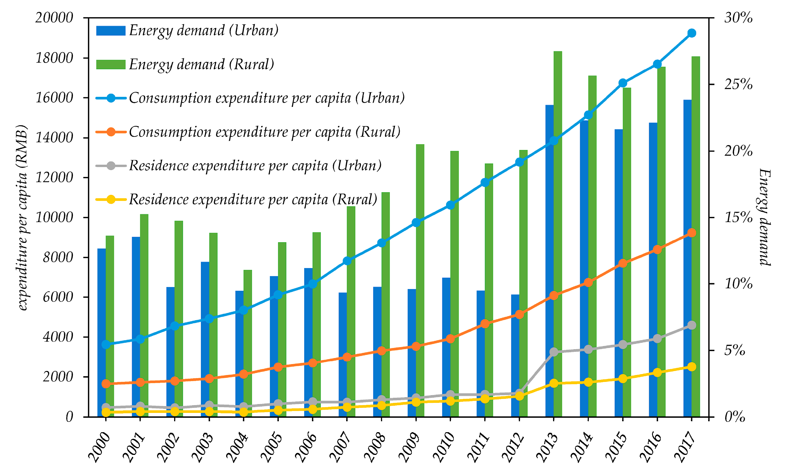
Therefore, simply stated, these results implicated that the effect of consumption expenditure was the first promoting factor to residential energy-related CO₂ emissions for both urban and rural residents, which was in line with the previous studies [9,17]. In fact, with the development of Jiangxi’s economy, both urban and rural residents’ living standards had greatly improved. Specifically, the consumption expenditure per capita of urban and rural residents increased from 3623.52 RMB and 1642.66 RMB in 2000 to 19244.46 RMB and 9230.21 RMB in 2017 (Figure 7), with a growth rate of 10.32% and 10.69%, respectively. As a result, people had the capacity to shift their consumption patterns to buy more appliances and transport tools, resulting in more energy consumption and CO₂ emissions. According to Pachauri [50], future increases in expenditure levels will lead to further increases in household energy requirement, in turn, a further increase in the urban and rural residential energy-related CO₂ emissions caused by the steady increase of the consumption expenditure per capita in Jiangxi in the future.

3.2.2. Energy Demand (ED)

It could be intuitively observed that the additive decomposition effect of energy demand was –73.42 × 10⁴ t and –0.11 × 10⁴ t in urban regions (Figure 5a and Table A3), exerting a negative effect on decreasing the urban residential energy-related CO₂ emissions during the first and second stages. However, the negative effect weakened year by year. This situation was mainly because the energy consumption growth lagged behind the growth of the consumption expenditure. However, during the third and fourth stages, the decomposition effect increased to 597.57 × 10⁴ t and 98.05 × 10⁴ t (Figure 5a and Table A3), respectively. This could be attributable to the rapid growth of the energy demand, which increased from 10.45% in 2010 to 21.64% in 2015, and then to 23.85% in 2017 (Figure 7). In total, the effect of energy demand made the second-largest contribution to the total annual average rate of urban residential CO₂ emissions (6.77%), and for each of the four stages, the corresponding average annual contribution rates were –2.72%, –0.01%, 16.82% and 5.29%, respectively (Table 6). Overall, the energy demand effect played a key role in increasing the urban residential energy-related CO₂ emissions although it slightly mitigated the CO₂ emissions in Stage 1 and 2 (Figure 6 and Table A5).

Similarly, energy demand also had a positive effect on promoting the rural residential energy-related CO₂ emissions over the study period (Figure 6 and Table A6). In total, it contributed to 427.17 × 10⁴ t CO₂ emissions, with an annual average contribution rate of 11.96% (Figure 5b and Table 7). Compared to urban regions, the energy demand exerted a positive effect on increasing the rural residential energy-related CO₂ emissions except Stage 1 (–25.50 × 10⁴ t), which contributed to 233.69 × 10⁴ t, 140.46 × 10⁴ t and 78.52 × 10⁴ t in Stage 2, 3 and 4 (Figure 5b and

Table A4. Rural, LMDI additive: Detailed additive decomposition results of the residential energy-related CO₂ emissions of rural residents in Jiangxi (10⁴ t).

Periods	$\mathsf{\Delta }{\mathbf{C}}_{\mathbf{T}\mathbf{O}\mathbf{T}}$	$\mathsf{\Delta }{\mathbf{C}}_{\mathbf{K}}$	$\mathsf{\Delta }{\mathbf{C}}_{\mathbf{E}\mathbf{S}}$	$\mathsf{\Delta }{\mathbf{C}}_{\mathbf{E}\mathbf{P}}$	$\mathsf{\Delta }{\mathbf{C}}_{\mathbf{E}\mathbf{D}}$	$\mathsf{\Delta }{\mathbf{C}}_{\mathbf{C}\mathbf{P}}$	$\mathsf{\Delta }{\mathbf{C}}_{\mathbf{U}}$	$\mathsf{\Delta }{\mathbf{C}}_{\mathbf{P}}$
2000–2001	115.71	7.00	−7.15	82.19	29.35	11.99	−9.99	2.33
2001–2002	40.89	−4.12	−18.94	68.94	−11.64	12.55	−8.87	2.97
2002–2003	68.72	2.41	23.17	49.52	−25.06	26.52	−10.83	2.99
2003–2004	22.88	12.32	41.35	26.57	−96.27	46.15	−10.15	2.92
2004–2005	112.61	2.58	1.92	−31.81	78.12	69.63	−10.72	2.89
2005–2006	−29.35	−27.58	32.88	−99.08	30.99	43.95	−14.09	3.57
2006–2007	26.62	2.46	13.72	−106.71	67.78	55.39	−9.48	3.46
2007–2008	−4.51	−4.55	15.02	−97.22	36.53	56.45	−14.83	4.08
2008–2009	51.68	−11.23	15.51	−91.10	114.32	38.48	−18.57	4.27
2009–2010	24.69	−0.93	2.51	−19.22	−15.93	63.78	−9.77	4.23
2010–2011	15.68	0.11	5.22	−55.89	−30.75	112.32	−19.09	3.75
2011–2012	−2.01	−63.95	16.55	−31.14	33.69	62.72	−22.14	2.25
2012–2013	77.76	35.91	−46.11	−231.22	217.66	116.89	−18.14	2.79
2013–2014	31.19	−19.24	−11.31	54.47	−52.03	75.98	−19.97	3.30
2014–2015	58.97	−29.65	−0.58	31.21	−28.11	104.32	−22.26	4.02
2015–2016	42.90	−28.26	7.12	−40.17	52.19	73.26	−26.13	4.89
2016–2017	90.28	25.87	−2.03	−23.13	26.33	86.90	−29.53	5.88
2000–2005	360.81	20.19	40.35	195.41	−25.50	166.83	−50.56	14.09
2005–2010	69.11	−41.83	79.65	−413.33	233.69	258.04	−66.74	19.62
2010–2015	181.59	−76.82	−36.24	−232.56	140.46	472.22	−101.60	16.11
2015–2017	133.18	−2.39	5.09	−63.31	78.52	160.16	−55.66	10.77
2000–2017	744.69	−100.84	88.84	−513.78	427.17	1057.26	−274.55	60.59

), respectively. This was because the energy demand decreased from 13.63% in 2000 to 13.13% in 2005, then it increased to 20.01% in 2010 and 27.12% in 2017 (Figure 7).

3.2.3. Population (P)

It was apparent the effect of population was the most stable and negligible factor to promote the urban and rural residential energy-related CO₂ emissions (Table A5 and Table A6), which was consistent with the previous studies [11,20]. Specifically, the average annual promoting impact of population effect (0.76% for urban, 1.70% for rural) was much lower than those of consumption expenditure per-capita effect and energy demand effect (Table 6 and Table 7). See from urban and rural, at each of four stages, the additive decomposition effects were 19.25 × 10⁴ t, 20.06 × 10⁴ t, 18.29 × 10⁴ t and 12.14 × 10⁴ t for urban residents (Figure 5a and Table A3), similarly, 14.09 × 10⁴ t, 19.62 × 10⁴ t, 16.11 × 10⁴ t and 10.77 × 10⁴ t for rural regions (Figure 5b and Table A4). Over the study period, it could be found the population effect presented an inverted U-shape trend in urban and rural regions, implying the population effect would weaken in the future. The total population increased from 41.49 million to 46.22 million, with an annual growth rate of only 0.64% in Jiangxi over this 17-year period (Figure 8). In fact, to the best of our knowledge, population was a stable element for a region during a certain period, i.e., population would increase with a stable growth rate.

3.2.4. Urbanization (U)

The additive decomposition results of urbanization in urban regions were 145.86 × 10⁴ t, 98.97 × 10⁴ t, 125.77 × 10⁴ t and 55.32 × 10⁴ t at each of four stages (Figure 5a and Table A3), indicating the effect of urbanization always had a positive influence on increasing the urban residential energy-related CO₂ emissions. The results were consonance with the results in Table A5. In total, the effect of urbanization made a specific contribution to the total urban residential energy-related CO₂ emissions growth (4.64%) (Table 6). Compare to urban regions, the additive decomposition results of urbanization effect in rural regions were –50.56 × 10⁴ t, –66.74 × 10⁴ t, –101.60 × 10⁴ t and –55.66 × 10⁴ t during the four stages (Figure 5b and Table A4), respectively. Eventually, the urbanization effect led to the total rural residential energy-related CO₂ emissions decrease at an annual average rate of 7.69% (Table 7). Overall, the results showed the urbanization effect was the inhibiting factor to the rural residential energy-related CO₂ emissions (Table A6). The difference between urban and rural regions could be explained by the followings.

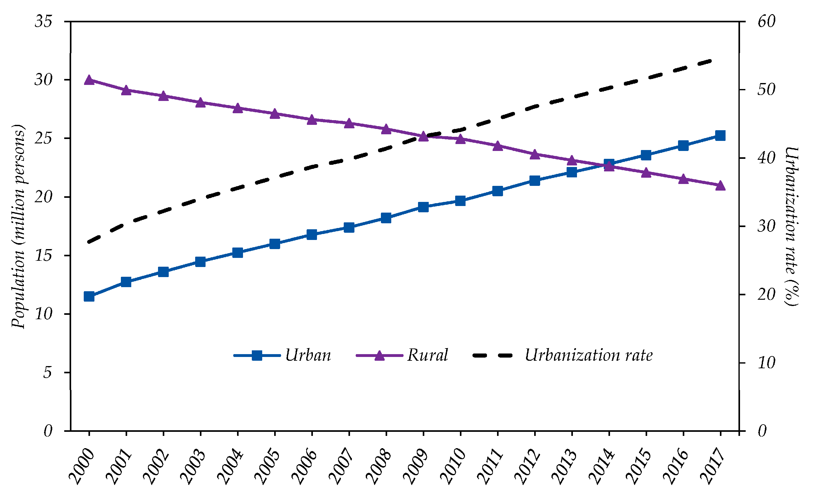
As depicted in Figure 8, the population of urban residents increased from 11.49 million to 25.24 million with an annual growth rate of 4.74%, and the population of rural residents decreased from 30.00 million to 20.98 million with an annual change of –2.08%. Correspondingly, the urbanization rate steadily increased from 27.69% to 54.6% from 2000–2017. In light of the context mentioned above, the urbanization effect increased the urban residential energy-related CO₂ emissions, but decreased the rural residential energy-related CO₂ emissions. On average, when the urbanization increased by 1%, the urban residential energy-related CO₂ emissions might have a growth of about 15.83 × 10⁴ t, while the rural residential energy-related CO₂ emissions might have a reduction of about 10.20 × 10⁴ t. See from each of four stages, the annual average contribution rates were 5.40%, 3.61%, 3.54% and 2.99% in urban regions (Table 6), and –4.81%, –2.34%, –3.17% and –3.39% in rural regions (Table 7). The urbanization effect presented a decline trend on the whole. In the future, this effect might be offset with the further development of Jiangxi’s urbanization. It was demonstrated by the contribution rate of the urbanization effect in Guangdong, the most developed province of China, experienced an increase trend to 53.6% in 2003, then declined to 17.3% in 2012 with a diminishing trend over time [21]. Furthermore, Fan, et al. [19] also pointed out the urbanization contributed to the increase to Chinese residential energy consumption but with a diminishing trend over time.

3.2.5. Energy Structure (ES)

Energy structure adjustment played a minor role in increasing the residential energy-related CO₂ emissions in urban and rural regions (Table A5 and Table A6), which was consistent with most relevant studies [21,51]. Over the study period, the aggregate changes of the energy structure effect were 94.29 × 10⁴ t and 88.84 × 10⁴ t (Figure 5), and the corresponding average annual contribution rates were 1.03% and 2.49%, respectively. Specifically, in the four stages, the corresponding annual average contribution rates were 6.34%, –2.23%, –0.82%, 0.72% for urban regions (Table 6), and 3.84%, 2.79%, –1.13% and 0.31% for rural regions (Table 7). The usage of coal steadily decreased in both urban and rural regions, resulting in the share of the residential energy-related CO₂ emissions decreased to 5.90%, 27.52% in 2017 from 60.06%, 73.59% in 2000 (Figure 4). However, the share of residential energy-related CO₂ emissions caused by oil and electricity rapidly increased, especially electricity. Furthermore, the share of natural gas was still low in Jiangxi, especially in rural regions. It was worth mentioning that the source endowment of China (including Jiangxi) was dominated by coal in the long term, and the electricity generation was mainly from coal [9,52]. The renewable and sustainable energy, such as wind, solar, nuclear, and biomass energy, had not been widely used [36]. Thus, it still required a longer time to thoroughly shift the energy structure to the low-carbon pattern to reduce the residential energy-related CO₂ emissions.

3.2.6. Energy Price (EP)

The energy price effect had the most important impact lowering the residential CO₂ emissions in urban and rural regions over the study period (Table A5 and Table A6), which was consistent with the previous studies [10,21]. Specifically, the additive decomposition effects were –549.64 × 10⁴ t, –152.25 × 10⁴ t, –782.11 × 10⁴ t and –128.61 × 10⁴ t for urban regions (Figure 5a and Table A3), the corresponding average annual contribution rates were –20.34%, –5.55%, –22.02% and –6.95%, respectively (Table 6). Similarly, in rural regions, the energy price effect led to 195.41 × 10⁴ t CO₂ emissions from 2000–2005. However, the decomposition effect decreased greatly to –413.33 × 10⁴ t, –232.56 × 10⁴ t and –63.31 × 10⁴ t during Stage 2, 3 and 4 (Figure 5b and Table A4), respectively, and for each of the four stages, the average annual contribution rates were 18.60%, –14.48%, –7.27% and –3.85%, respectively (Table 7).

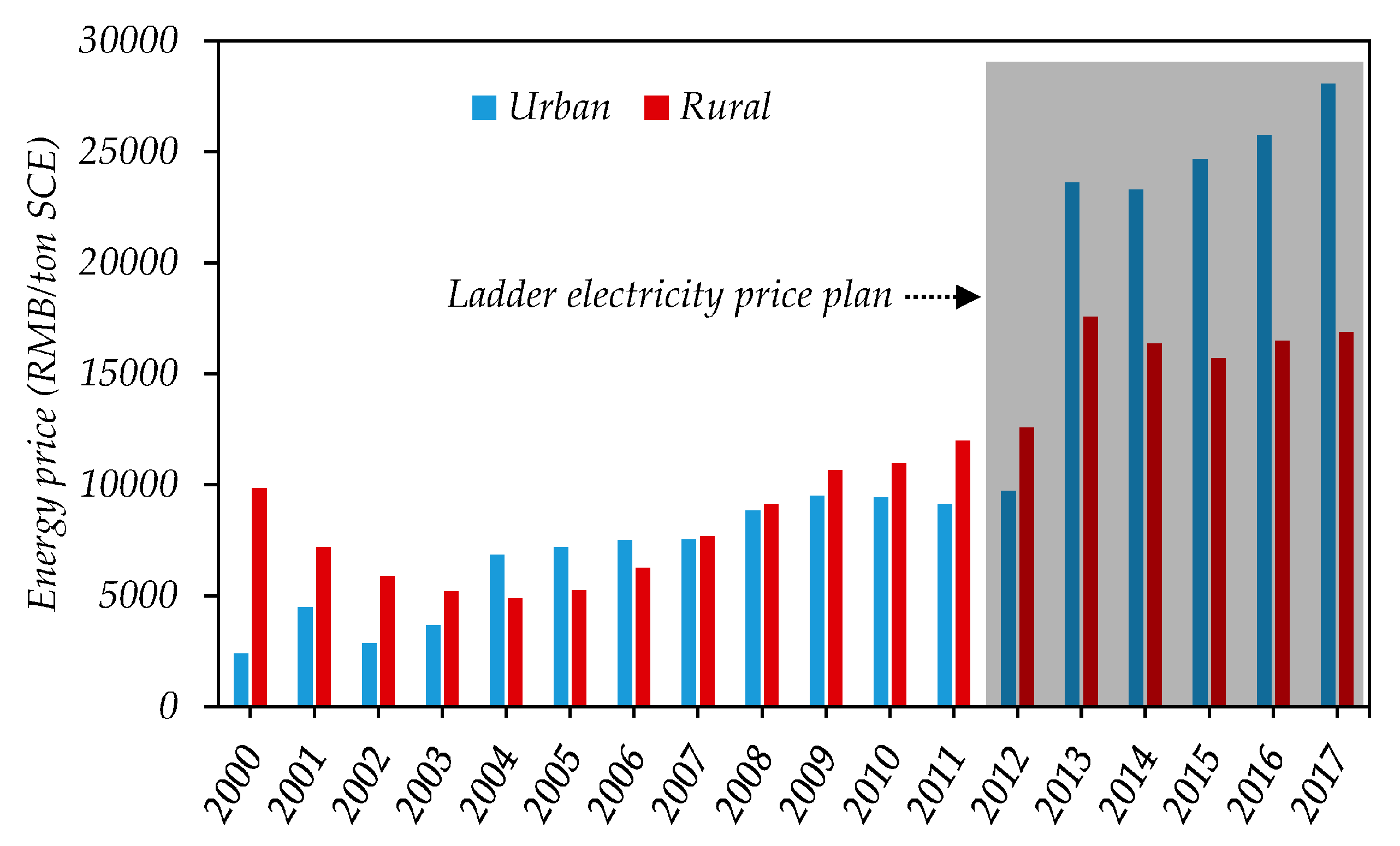
Overall, the energy price effect made the greatest contribution to the total annual rates of urban and rural residential energy-related CO₂ emissions mitigation (–17.55% for urban and –14.38% for rural) (Table 6 and Table 7). This was mainly because the energy price increased from 2410.53 RMB/ ton-standard coal equivalent (SCE), 9855.43 RMB/ ton SCE in 2000 to 28078.53 RMB/ ton SCE, 16900.13 RMB/ ton SCE in 2017 for urban and rural regions, respectively (Figure 9), restraining the willing of people’s consumption. In particular, it should be noted that the energy price rapidly grew from 9730.42 RMB/ ton SCE in 2012 to 24690.65 RMB/ ton SCE in 2015 because of the implementation of the “ladder electricity price plan (In November 2011, the National Development and Reform Commission (NDRC) issued the “residential ladder electricity price policy” to promote energy conservation and emission reduction as well as social equity. Specifically, residential electricity consumption was divided into three grades and a free grade for low-income households.)” in Jiangxi urban regions, making the energy price reached the peak value (–782.11 × 10⁴ RMB/ton SCE). Moreover, during Stage 1, the energy price decreased from 9855.43 RMB/ ton SCE to 5226.89 RMB/ ton SCE, which stimulated the consumption of rural residents.

3.2.7. Carbon Emission Coefficient (K)

As mentioned above, in this article, the carbon emission coefficient of electricity was not a constant value. The carbon emission coefficient effect mainly derived from the change of the carbon emission coefficient of power generation (Table A1). In addition, according to Ren, et al. [53], if the contribution of the energy emission factor was negative, the residential energy-related CO₂ emissions decreased. Otherwise, the contribution of the energy emission factor was positive and the residential energy-related increased.

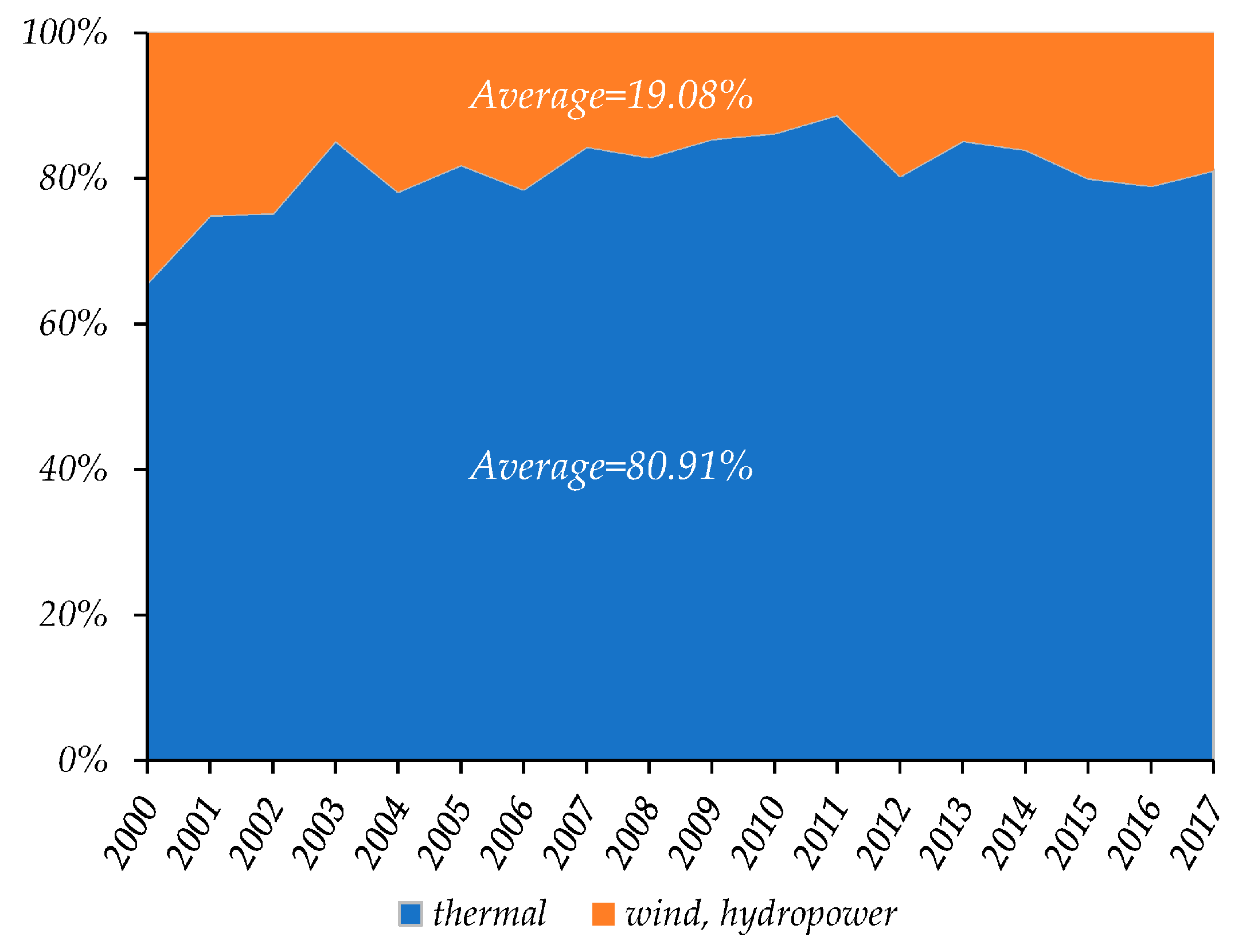
The carbon emission coefficient effect had the least influence on inhibiting the residential energy-related CO₂ emissions in both urban and rural regions (Table A5 and Table A6). In total, the average annual contribution rates were –1.17% and –2.82% for urban and rural regions (Table 6 and Table 7), respectively. See from each of four stages, the corresponding contribution rates were 1.36% and 1.92% in urban and rural regions from 2000–2005, indicating the carbon emission coefficient effect had a minor influence on increasing the CO₂ emissions. This situation was likely that the carbon emission coefficient of electricity increased from 6.49 t-CO₂/10⁴ kwh to 7.99 t-CO₂/10⁴ kwh in Jiangxi (Table A1). However, in 2005–2010, 2010–2015, and 2015–2017, the average annual contribution rates decreased to –2.32%, –2.22%, –0.12% for urban regions, and –1.47%, –2.40%, –0.15% for rural regions, respectively. The results might be due to the improvement of power generation technology, updated generation equipment and other factors [53]. Specifically, the carbon emission coefficient of electricity decreased from 7.99 t-CO₂/10⁴ kwh to 4.84 t-CO₂/10⁴ kwh in 2017. On the other hand, the carbon emission coefficient effect represented an overall downward trend, resulting from the long-term coal-dependent power generation in Jiangxi (Average=80.91%) (Figure 10). Hence, the carbon emission coefficient effect eventually had a relatively marginal negative contribution to the residential energy-related CO₂ emissions reduction. To effectively enhance the effect of energy emission factor to mitigate CO₂ emissions, it is necessary to boost the share of cleaner energy types such as hydropower, wind power, and solar power in Jiangxi’s electricity generation structure.

3.3. Decoupling Analysis of Residential Energy-Related CO₂ Emissions at Four Stages

As shown in

Table 8. The decoupling state between residential energy-related CO₂ emissions and consumption expenditure in Jiangxi urban and rural regions over the study period.

Time Period	Urban				Rural
	C%	Y%	D	State	C%	Y%	D	State
2000–2001	−0.20	0.19	−1.04	SD	0.55	0.02	32.89	END
2001–2002	0.32	0.25	1.29	END	0.13	0.02	6.36	END
2002–2003	0.14	0.15	0.92	EC	0.19	0.05	3.90	END
2003–2004	−0.41	0.14	−2.82	SD	0.05	0.10	0.55	WD
2004–2005	0.42	0.20	2.09	END	0.25	0.15	1.66	END
2005–2006	0.03	0.14	0.19	WD	−0.05	0.06	−0.83	SD
2006–2007	0.02	0.22	0.11	WD	0.05	0.10	0.49	WD
2007–2008	0.01	0.17	0.05	WD	−0.01	0.08	−0.09	SD
2008–2009	0.06	0.17	0.33	WD	0.09	0.04	2.19	END
2009–2010	0.15	0.12	1.29	END	0.04	0.10	0.41	WD
2010–2011	0.09	0.15	0.56	WD	0.02	0.16	0.15	WD
2011–2012	−0.02	0.13	−0.15	SD	0.00	0.07	−0.05	SD
2012–2013	0.16	0.12	1.34	END	0.12	0.16	0.75	WD
2013–2014	0.03	0.13	0.27	WD	0.04	0.08	0.52	WD
2014–2015	0.02	0.14	0.15	WD	0.08	0.12	0.66	WD
2015–2016	0.05	0.09	0.57	WD	0.05	0.06	0.82	EC
2016–2017	0.14	0.13	1.12	EC	0.10	0.07	1.45	END
2000–2005	0.01	1.35	0.01	WD	1.72	0.37	4.68	END
2005–2010	0.30	1.14	0.26	WD	0.12	0.45	0.27	WD
2010–2015	0.30	0.89	0.34	WD	0.28	0.74	0.38	WD
2015–2017	0.20	0.23	0.87	EC	0.16	0.14	1.15	EC
2000–2017	1.06	10.67	0.10	WD	3.54	2.93	1.21	END

Note: C% and Y% denote change rates of residential energy-related CO₂ emissions and consumption expenditure, respectively; D denotes the results of decoupling indicators.

, four decoupling states occurred in Jiangxi urban regions, namely SD, END, WD, and EC. From 2000–2005, the decoupling states switched every year, thereby implying that an unstable relationship between urban residential energy-related CO₂ emissions and consumption expenditure. Eventually, the decoupling state showed WD, that is to say, the consumption expenditure increased a little faster than the CO₂ emissions. After 2005, the decoupling states converged on the WD in most years of the period 2005–2016, except 2009–2010 and 2012–2013. Furthermore, the decoupling state was EC in the end, suggesting that there is no significant relationship between the CO₂ emissions and consumption expenditure. Overall, the decoupling states were the WD, WD, and EC from 2005–2010, 2010–2015, and 2015–2017, respectively. Over the study period, the decoupling state was WD in Jiangxi urban regions.

Table 8 also presented the decoupling state of Jiangxi rural regions. Similarly, there are also four types of decoupling states: END, SD, WD, and EC. However, there are some differences. Specifically, the decoupling states were stable and converged on END from 2000–2005. Meanwhile most years of the period 2005–2015, the decoupling states mainly converged on WD and SD, except 2008–2009 (END). This caused the decoupling state shift from END in 2000–2005 to WD in 2005–2010 and 2010–2015. In the later period (2015–2017), the decoupling state was EC, resulting from the unsatisfactory decoupling states in 2015–2016 (EC) and 2016–2017 (END). Simply stated, the decoupling state in Jiangxi rural regions showed the END over the study period. Compared to the urban regions, the decoupling process needed further to accelerate in Jiangxi rural regions.

During Stage 1 (2000–2005), both urban and rural residents’ income increased with the development of economy. Correspondingly, the consumption expenditure grew by 135% and 37% (Table 8), respectively. To ensure the quick development of economy, the demand for urban residents was restrained, which caused the residential energy-related CO₂ emissions increased by only 1%. Thus, the consumption expenditure increased much greater than the CO₂ emissions, leading to an overall WD (0.01) in Stage 1 although EC and END occurred in 2001–2003 and 2004–2005 (Table 8). See from rural, decline of energy price stimulated the residents’ consumption desire which made the energy demand increase (Figure 7). Meanwhile, it caused the CO₂ emissions rose by 172% in 2000–2005 which was greatly higher than that of consumption expenditure. Consequently, the decoupling state was END in this stage.

During Stage 2 (2005–2010), the consumption expenditure rose by 114% (Table 8), which made urban residents pursuit more high-quality life and buy more high-carbon appliance and family cars (Table 4). Thus, the CO₂ emissions grew by 30%, presenting the WD (0.26) (Table 8) in 2005–2010. As to rural residents, on one hand, rural residential consumption expenditure further rose by 45%. On the other hand, traditional outdated energy gradually placed by the commercial energy in Jiangxi rural regions and the CO₂ emissions increased by 12%. As a result, the decoupling state shifted from END to WD in Stage 2.

During Stage 3 (2010–2015), both urban and rural regions presented WD. The growth rate of the consumption expenditure continued to slow down and grew by 89% in urban regions. However, it continued to rise and grew by 74% in rural regions (Table 8). This could be explained by the long-term inequality and lag between urban and rural regions in China’s economic development (including Jiangxi), namely duality of urban–rural. Moreover, in order to save energy and reduce emissions, Chinese government (Jiangxi included) formulated and implemented the “ladder electricity price policy” after 2012, which effectively restrained residential energy consumption, especially in urban regions. Thus, the change rate of the CO₂ emissions in urban regions nearly had no obvious increase (30% from 2010–2015), and it grew by 28% in rural regions. Consequently, WD occurred.

During Stage 4 (2015–2017), the relationship between consumption expenditure and residential energy-related CO₂ emissions transformed from WD to EC in both urban and rural regions. Chinese economic development embarked on a new stage called “the new normal”. Specifically, in this stage, China (including Jiangxi) shifted its development pattern from rapid growth to more inclusive and sustainable growth, including higher living standards, cleaner production [54]. Consequently, the growth rate of consumption expenditure and the CO₂ emissions declined, to some extent. Consumption expenditure rose by 23% and 14% in Jiangxi urban and rural regions (Table 8), respectively, which was slower than that of other periods. Additionally, the CO₂ emissions also showed a decline trend and grew by 20% and 16% in Jiangxi urban and rural regions, resulting from the improvement of energy efficiency. Therefore, they both presented EC in this stage, indicating there was insignificant decoupling between consumption expenditure and the CO₂ emissions.

4. Conclusions and Policy Implications

4.1. Main Conclusions

Presently, residential energy consumption has become the second-largest sector to the industrial energy consumption in China. However, little attention was paid to research the difference of the residential energy-related CO₂ emissions between urban and rural areas in the less developed and undeveloped regions. Thus, based on the urban–rural duality, this paper aims at exploring the difference of the residential energy-related CO₂ emissions in Jiangxi urban and rural regions from 2000–2017. We first overviewed the changes of the residential energy-related CO₂ emissions in Jiangxi between urban and rural regions. Then, the LMDI method was introduced to distinguish the major factors affecting the residential energy-related CO₂ emissions. In addition, the Tapio decoupling model was used to analyze the relationship between residential energy-related CO₂ emissions and consumption expenditure. The main results were acquired as follows.

The residential energy-related CO₂ emissions rapidly increased after 2008 in both Jiangxi urban and rural regions. However, the annual growth rate of urban regions (7.47%) was faster than rural regions (6.03%). In addition, the gap between urban and rural regions became narrowed and stable. The energy structures of both urban and rural residential energy-related CO₂ emissions had shifted from coal-dominant to a multiple structure which consisted of oil, natural gas, and electricity. Specifically, the energy-related CO₂ emissions structure was electricity, oil, natural gas, and coal in sequence for urban; it was electricity, coal, oil, and natural gas in sequence for rural. As for the residential energy-related CO₂ emissions per capita, it showed a decline trend in urban regions, while an increasing tendency in rural regions over the study period. The gap in residential energy-related CO₂ emissions for urban and rural residents narrowed from 2000–2007.

The energy price effect played the most important role in reducing the residential energy-related CO₂ emissions in both urban and rural regions. In addition, the carbon emission coefficient had a minor effect on decreasing urban and rural residential energy-related CO₂ emissions. The results showed that urbanization exerted a positive effect on increasing the urban residential energy-related CO₂ emissions, but decreasing the rural residential energy-related CO₂ emissions. Consumption expenditure-per-capita effect was the most important factor increasing the residential energy-related CO₂ emissions in both urban and rural regions, followed by energy demand. From 2000–2017, population effect and energy structure played a minor role in increasing the urban and rural residential energy-related CO₂ emissions.

Over the study period, four decoupling status (END, SD, WD, and EC) occurred in both urban and rural regions when analyzed the relationship between consumption expenditure and residential energy-related CO₂ emissions. Overall, the decoupling state for urban and rural regions were the WD and END. This showed that residential energy-related CO₂ emissions in urban Jiangxi was less depend on consumption expenditure, but rural residential energy-related CO₂ emissions still depended on consumption expenditure.

4.2. Policy Implications

First, since the residential energy-related CO₂ emissions caused by coal was still high in rural regions, which accounted for 27.52% and was second only to electricity (53.78%) even in 2017. However, the corresponding proportion of natural gas was always low and took up less than 1% over the study period. Thus, the energy structure of rural regions had more space to optimize, and more efforts should be paid to further adjust the rural energy structure. For instance, promoting the proportion of natural gas and encouraging the use of renewable and clean energy in rural regions.

Second, since the rural residential energy-related CO₂ emissions per capita had exceeded that of the urban region after 2015, thereby suggesting that the lifestyles in rural regions were more extensive and lower energy efficiency compared with urban regions. On one hand, it is urgent and imperative for the government at all levels to strengthen related public education and guide residents to shift their high-carbon lifestyles to a green and low-carbon pattern, especially for rural residents. In addition, the government should accelerate the elimination of backward production capacity to improve the efficiency in rural regions. On the other hand, residents themselves should also initiatively adapt to the transformation and cultivate the awareness of environmental protection.

Third, consumption expenditure-per-capita effect became the most factor increasing the residential energy-related CO₂ emissions in both urban and rural regions. With the improvement of economic growth and living standards, people had the desire and capacity to pursuit the quality of life and buy more energy-intensive electricity appliances and private transport tools. However, it is not wise to reduce the CO₂ emissions via restraining the consumption, this was because the consumption was a critical impetus of socio-economic development. Thus, the government could apply the fiscal and tax policy to cut down the residential energy-related CO₂ emissions and accelerate the decoupling. Specifically, the government should continue to impose the “Home Appliances Subsidy Program” and monitor its proper extent of implementation. For the high-carbon and extensive goods and services, the government could add the tax to restrain the CO₂-intensive commodities’ consumption. Meanwhile for the energy-saving appliances, reducing the tax could stimulate the low-carbon consumption. Moreover, more investment and efforts were needed to improve public transport infrastructures and the energy conservation technology.

Fourth, considering energy price played the most important role in decreasing the residential energy-related CO₂ emissions in both urban and rural regions, indicating tiered energy price was the effective and scientific pathway to achieve energy savings and emissions reduction. In light of the fact, the government needs further to uphold and ameliorate the energy price policy in the future. In particular, when applying the energy price mechanism, the duality as well as inequality of income level and economic development should be comprehensively considered in urban and rural regions.

Last, to the best of our knowledge, residential building energy consumption accounted for a large proportion of the total residential energy consumption, leading to enormous CO₂ emissions. Therefore, it is necessary to improve residential building energy efficiency, especially for rural regions. For urban regions, the intelligent energy management technology in household could be popularized and applied to achieve energy conservation.

5. Limitations and Further Perspectives

There are limitations to this study. Based on the perspective of end-use of energy, only the residential energy-related CO₂ emissions were estimated, while the indirect or embodied residential CO₂ emissions from production perspective were excluded. This could likely underestimate the residential CO₂ emissions in Jiangxi urban and rural regions. Therefore, the embodied residential CO₂ emissions need further study. Moreover, this paper only explored the factors affecting the residential energy-related CO₂ emissions and the decoupling relationship between consumption expenditure and residential energy-related CO₂ emissions in Jiangxi urban and rural regions, specifically carbon emission coefficient, energy structure, consumption expenditure per capita, energy demand, energy price, urbanization, and population. However, family size, floor space of residential buildings and different income levels (an aspect of social inequality) also had the nonnegligible effect on the residential CO₂ emissions. Thus, these influencing factors to the residential CO₂ emissions should be paid more attention in our future work.

References

1. Fan, J.-L.; Yu, H.; Wei, Y.-M. Residential energy-related carbon emissions in urban and rural China during 1996–2012: From the perspective of five end-use activities. Energy Build. 2015, 96, 201–209. [Google Scholar] [CrossRef]
2. IPCC. Climate Change 2007: IPCC Fourth Assessment Report; Cambridge University Press: Cambridge, UK, 2007. [Google Scholar]
3. Mi, Z.; Meng, J.; Guan, D.; Shan, Y.; Liu, Z.; Wang, Y.; Feng, K.; Wei, Y.-M. Pattern changes in determinants of Chinese emissions. Environ. Res. Lett. 2017, 12, 074003. [Google Scholar] [CrossRef]
4. Guan, D.; Meng, J.; Reiner, D.M.; Zhang, N.; Shan, Y.; Mi, Z.; Shao, S.; Liu, Z.; Zhang, Q.; Davis, S.J. Structural decline in China’s CO2 emissions through transitions in industry and energy systems. Nat. Geosci. 2018, 11, 551–555. [Google Scholar] [CrossRef]
5. Lin, B.; Liu, K. Using LMDI to analyze the decoupling of carbon dioxide emissions from China’s heavy industry. Sustainability 2017, 9, 1198. [Google Scholar]
6. Fan, J.-L.; Liao, H.; Liang, Q.-M.; Tatano, H.; Liu, C.-F.; Wei, Y.-M. Residential carbon emission evolutions in urban–rural divided China: An end-use and behavior analysis. Appl. Energy 2013, 101, 323–332. [Google Scholar] [CrossRef]
7. Zhang, X.; Luo, L.; Skitmore, M. Household carbon emission research: An analytical review of measurement, influencing factors and mitigation prospects. J. Clean. Prod. 2015, 103, 873–883. [Google Scholar] [CrossRef] [Green Version]
8. Huang, R.; Zhang, S.; Liu, C. Comparing urban and rural household CO2 emissions—Case from China’s four megacities: Beijing, Tianjin, Shanghai, and Chongqing. Energies 2018, 11, 1257. [Google Scholar] [CrossRef] [Green Version]
9. Tian, X.; Geng, Y.; Dong, H.; Dong, L.; Fujita, T.; Wang, Y.; Zhao, H.; Wu, R.; Liu, Z.; Sun, L. Regional household carbon footprint in China: A case of Liaoning province. J. Clean. Prod. 2016, 114, 401–411. [Google Scholar] [CrossRef]
10. Shi, Y.; Han, B.; Han, L.; Wei, Z. Uncovering the national and regional household carbon emissions in China using temporal and spatial decomposition analysis models. J. Clean. Prod. 2019, 232, 966–979. [Google Scholar] [CrossRef]
11. Zhu, Q.; Peng, X.; Wu, K. Calculation and decomposition of indirect carbon emissions from residential consumption in China based on the input–output model. Energy Policy 2012, 48, 618–626. [Google Scholar] [CrossRef]
12. Lu, Y.; Zhang, Y.; Cao, X.; Wang, C.; Wang, Y.; Zhang, M.; Ferrier, R.C.; Jenkins, A.; Yuan, J.; Bailey, M.J.; et al. Forty years of reform and opening up: China’s progress toward a sustainable path. Sci. Adv. 2019, 5, 9413–9422. [Google Scholar] [CrossRef] [PubMed] [Green Version]
13. Yang, L.; Yang, Y.; Zhang, X.; Tang, K. Whether China’s industrial sectors make efforts to reduce CO2 emissions from production?—A decomposed decoupling analysis. Energy 2018, 160, 796–809. [Google Scholar] [CrossRef]
14. Zha, D.; Zhou, D.; Zhou, P. Driving forces of residential CO2 emissions in urban and rural China: An index decomposition analysis. Energy Policy 2010, 38, 3377–3383. [Google Scholar]
15. Fan, J.; Ran, A.; Li, X. A study on the factors affecting China’s direct household carbon emission and comparison of regional differences. Sustainability 2019, 11, 4919. [Google Scholar] [CrossRef] [Green Version]
16. Feng, Z.-H.; Zou, L.-L.; Wei, Y.-M. The impact of household consumption on energy use and CO2 emissions in China. Energy 2011, 36, 656–670. [Google Scholar] [CrossRef]
17. Liu, L.-C.; Wu, G.; Wang, J.-N.; Wei, Y.-M. China’s carbon emissions from urban and rural households during 1992–2007. J. Clean. Prod. 2011, 19, 1754–1762. [Google Scholar] [CrossRef]
18. Bai, Y.; Deng, X.; Gibson, J.; Zhao, Z.; Xu, H. How does urbanization affect residential CO2 emissions? An analysis on urban agglomerations of China. J. Clean. Prod. 2019, 209, 876–885. [Google Scholar] [CrossRef]
19. Fan, J.-L.; Zhang, Y.-J.; Wang, B. The impact of urbanization on residential energy consumption in China: An aggregated and disaggregated analysis. Renew. Sust. Energ. Rev. 2017, 75, 220–233. [Google Scholar] [CrossRef]
20. Ye, Y.; Shi, X.-Q.; Zou, L.-L. Decoupling economic growth from CO2 emissions: A decomposition analysis of China’s household energy consumption. Adv. Clim. Chang. Res. 2016, 7, 192–200. [Google Scholar]
21. Wang, W.; Zhao, D.; Kuang, Y. Decomposition analysis on influence factors of direct household energy-related carbon emission in Guangdong province-Based on extended Kaya identity. Environ. Prog. Sustain. Energy 2016, 35, 298–307. [Google Scholar] [CrossRef] [Green Version]
22. Yuan, R.; Rodrigues, J.F.D.; Behrens, P. Driving forces of household carbon emissions in China: A spatial decomposition analysis. J. Clean. Prod. 2019, 233, 932–945. [Google Scholar] [CrossRef]
23. Zhang, M.; Bai, C. Exploring the influencing factors and decoupling state of residential energy consumption in Shandong. J. Clean. Prod. 2018, 194, 253–262. [Google Scholar] [CrossRef]
24. Nie, H.; Kemp, R. Index decomposition analysis of residential energy consumption in China: 2002–2010. Appl. Energy 2014, 121, 10–19. [Google Scholar] [CrossRef]
25. Zhang, M.; Song, Y.; Li, P.; Li, H. Study on affecting factors of residential energy consumption in urban and rural Jiangsu. Renew. Sust. Energ. Rev. 2016, 53, 330–337. [Google Scholar] [CrossRef]
26. Ye, H.; Ren, Q.; Hu, X.; Lin, T.; Xu, L.; Li, X.; Zhang, G.; Shi, L.; Pan, B. Low-carbon behavior approaches for reducing direct carbon emissions: Household energy use in a coastal city. J. Clean. Prod. 2017, 141, 128–136. [Google Scholar] [CrossRef] [Green Version]
27. Zhao, X.; Li, N.; Ma, C. Residential energy consumption in urban China: A decomposition analysis. Energy Policy 2012, 41, 644–653. [Google Scholar] [CrossRef]
28. OECD. Indicators to Measure Decoupling of Environmental Pressure from Economic Growth; Organization for Economic Cooperation and Development (OECD): Paris, France, 2002. [Google Scholar]
29. Tapio, P. Towards a theory of decoupling: Degrees of decoupling in the EU and the case of road traffic in Finland between 1970 and 2001. Transp. Policy 2005, 12, 137–151. [Google Scholar] [CrossRef] [Green Version]
30. Wang, Q.; Li, R.; Jiang, R. Decoupling and decomposition analysis of carbon emissions from industry: A case study from China. Sustainability 2016, 8, 1059. [Google Scholar] [CrossRef] [Green Version]
31. Zhang, L.; Kou, C.; Zheng, J.; Li, Y. Decoupling analysis of CO2 emissions in transportation sector from economic growth during 1995–2015 for six cities in Hebei, China. Sustainability 2018, 10, 4149. [Google Scholar] [CrossRef] [Green Version]
32. Wang, Y.; Xie, T.; Yang, S. Carbon emission and its decoupling research of transportation in Jiangsu Province. J. Clean. Prod. 2017, 142, 907–914. [Google Scholar] [CrossRef]
33. Jiang, R.; Li, R. Decomposition and decoupling analysis of life-cycle carbon emission in China’s building Sector. Sustainability 2017, 9, 886. [Google Scholar] [CrossRef] [Green Version]
34. Wang, Q.; Zhao, M.; Li, R. Decoupling sectoral economic output from carbon emissions on city level: A comparative study of Beijing and Shanghai, China. J. Clean. Prod. 2019, 209, 126–133. [Google Scholar] [CrossRef]
35. Luo, Y.; Long, X.; Wu, C.; Zhang, J. Decoupling CO2 emissions from economic growth in agricultural sector across 30 Chinese provinces from 1997 to 2014. J. Clean. Prod. 2017, 159, 220–228. [Google Scholar] [CrossRef]
36. Zhao, X.; Zhang, X.; Li, N.; Shao, S.; Geng, Y. Decoupling economic growth from carbon dioxide emissions in China: A sectoral factor decomposition analysis. J. Clean. Prod. 2017, 142, 3500–3516. [Google Scholar] [CrossRef]
37. Statistic Bureau of Jiangxi. Jiangxi Statistical Yearbook; China Statistics Press: Beijing, China, 2001–2018. (In Chinese)
38. Jia, J.; Gong, Z.; Xie, D.; Chen, J.; Chen, C. Analysis of drivers and policy implications of carbon dioxide emissions of industrial energy consumption in an underdeveloped city: The case of Nanchang, China. J. Clean. Prod. 2018, 183, 843–857. [Google Scholar] [CrossRef]
39. IPCC. Gudielines for National Greenhouse Gas Inventories; Cambridge University Press: Cambridge, UK, 2006. [Google Scholar]
40. National Bureau of Statistics of China. China Energy Statistical Yearbook; China Statistics Press: Beijing, China, 2001–2018. (In Chinese)
41. Kennedy, C.; Steinberger, J.; Gasson, B.; Hansen, Y.; Hillman, T.; Havránek, M.; Pataki, D.; Phdungsilp, A.; Ramaswami, A.; Mendez, G.V. Greenhouse gas emissions from global cities. Environ. Sci. Technol. 2009, 43, 7297–7302. [Google Scholar] [CrossRef]
42. Ang, B.W. The LMDI approach to decomposition analysis: A practical guide. Energy Policy 2005, 33, 867–871. [Google Scholar] [CrossRef]
43. Ang, B.W.; Liu, N. Handling zero values in the logarithmic mean Divisia index decomposition approach. Energy Policy 2007, 35, 238–246. [Google Scholar] [CrossRef]
44. Ang, B.W. Decomposition analysis for policymaking in energy. Energy Policy 2004, 32, 1131–1139. [Google Scholar] [CrossRef]
45. Ang, B.W.; Liu, F.L.; Chew, E.P. Perfect decomposition techniques in energy and environmental analysis. Energy Policy 2003, 31, 1561–1566. [Google Scholar] [CrossRef]
46. Kaya, Y. Impact of Carbon Dioxide Emission Control on GNP Growth: Interpretation of Proposed Scenarios; IPCC Energy and Industry Subgroup, Response Strategies Working Group: Paris, France, 1990. [Google Scholar]
47. Shao, S.; Yang, L.; Gan, C.; Cao, J.; Geng, Y.; Guan, D. Using an extended LMDI model to explore techno-economic drivers of energy-related industrial CO2 emission changes: A case study for Shanghai (China). Renew. Sust. Energ. Rev. 2016, 55, 516–536. [Google Scholar] [CrossRef] [Green Version]
48. Omer, A.M. Energy, environment and sustainable development. Renew. Sust. Energ. Rev. 2008, 12, 2265–2300. [Google Scholar] [CrossRef]
49. Tian, X.; Chang, M.; Lin, C.; Tanikawa, H. China’s carbon footprint: A regional perspective on the effect of transitions in consumption and production patterns. Appl. Energy 2014, 123, 19–28. [Google Scholar] [CrossRef]
50. Pachauri, S. Household electricity access a trivial contributor to CO2 emissions growth in India. Nat. Clim. Chang. 2014, 4, 1073–1076. [Google Scholar] [CrossRef]
51. Shao, S.; Yang, L.; Yu, M.; Yu, M. Estimation, characteristics, and determinants of energy-related industrial CO2 emissions in Shanghai (China), 1994–2009. Energy Policy 2011, 39, 6476–6494. [Google Scholar] [CrossRef]
52. Wei, Y.-M.; Liu, L.-C.; Fan, Y.; Wu, G. China Energy Report (2008): CO2 Emission Research; Science Press: Beijing, China, 2008. (In Chinese) [Google Scholar]
53. Ren, S.; Fu, X.; Chen, X. Regional variation of energy-related industrial CO2 emissions mitigation in China. China Econ. Rev. 2012, 23, 1134–1145. [Google Scholar] [CrossRef]
54. Grubb, M.; Sha, F.; Spencer, T.; Hughes, N.; Zhang, Z.; Agnolucci, P. A review of Chinese CO2 emission projections to 2030: The role of economic structure and policy. Clim. Policy 2015, 15, S7–S39. [Google Scholar] [CrossRef] [Green Version]
Figure 1. Location of Jiangxi.
Sustainability 12 02000 g001
Figure 2. Trends of residential energy-related CO2 emissions in Jiangxi urban and rural regions.
Sustainability 12 02000 g002
Figure 3. Changes of residential energy-related CO2 emissions structure in Jiangxi urban and rural regions from 2000–2017. (a) Urban. (b) Rural.
Sustainability 12 02000 g003
Figure 4. Changes of residential energy-related CO2 emissions per capita in Jiangxi urban and rural regions from 2000–2017.
Sustainability 12 02000 g004
Figure 5. Factors affecting the residential energy-related CO2 emissions in Jiangxi urban and rural regions from 2000–2017. (a) Urban. (b) Rural.
Sustainability 12 02000 g005
Figure 6. Multiplicative decomposition results of the residential energy-related CO2 emissions in Jiangxi urban and rural regions in the four stages (a) 2000–2005. (b) 2005–2010. (c) 2010–2015. (d) 2015–2017.
Sustainability 12 02000 g006
Figure 7. Trends of consumption expenditure, residence expenditure and energy demand in Jiangxi over the study period; Energy demand denotes the share of residence expenditure to consumption expenditure.
Sustainability 12 02000 g007
Figure 8. Trends of urban and rural population in Jiangxi over the study period.
Sustainability 12 02000 g008
Figure 9. Energy price in urban and rural Jiangxi.
Sustainability 12 02000 g009
Figure 10. Energy types of power generation in Jiangxi.
Sustainability 12 02000 g010